A Feasible Community Detection Algorithm for Multilayer Networks

Abstract

As a more complicated network model, multilayer networks provide a better perspective for describing the multiple interactions among social networks in real life. Different from conventional community detection algorithms, the algorithms for multilayer networks can identify the underlying structures that contain various intralayer and interlayer relationships, which is of significance and remains a challenge. In this paper, aiming at the instability of the label propagation algorithm (LPA), an improved label propagation algorithm based on the SH-index (SH-LPA) is proposed. By analyzing the characteristics and deficiencies of the H-index, the SH-index is presented as an index to evaluate the importance of nodes, and the stability of the SH-LPA algorithm is verified by a series of experiments. Afterward, considering the deficiency of the existing multilayer network aggregation model, we propose an improved multilayer network aggregation model that merges two networks into a weighted single-layer network. Finally, considering the influence of the SH-index and the weight of the edge of the weighted network, a community detection algorithm (MSH-LPA) suitable for multilayer networks is exhibited in terms of the SH-LPA algorithm, and the superiority of the mentioned algorithm is verified by experimental analysis.

1. Introduction

Popular research in the field of network science is to mine hidden information under the network structure. Community detection is an important aspect of complex network research, and we can see the presence of the community in various fields, such as detecting the intensive group organization in a social network [1], the different muscle tissue composed by various genes found in the gene protein networks [2], and so on. However, effectively and accurately detecting the community structure for large-scale networks tends to be urgently addressed.

The community detection algorithms can be divided into non-overlapping community detection algorithms and overlapping community detection algorithms according to whether they contain overlapping communities or not. Non-overlapping community detection algorithm can be divided into the following categories. (1) The hierarchical clustering method defines the similarity or distance between network nodes by the topology of the given network, groups network nodes into a tree hierarchy by single-connection or full-connection hierarchical clustering, and cross-cuts the tree diagram according to actual needs to obtain the community structure. The most famous algorithm is the GN algorithm [3], which continuously deletes the edge in the network that has the maximum edge-betweenness with respect to all source nodes, and then the edge-betweenness number of the remaining edges relative to all source nodes in the network is recalculated, and the process is repeated until the network, all edges are deleted. (2) In the spectral clustering method, the objective is to find a method of dividing the nodes into disjoint sets by cutting the least-cut edges, such as the algorithm in [4,5]. (3) In the modularity optimization method, a modularity optimization function $Q$ is employed to describe the quality of the detected community. A larger $Q$ value indicates a better community structure, such as the FN algorithm [6] that each node in the initialization network is a single community, and then select the most value-added community q module to merge, finally the network is merged into a community, the algorithm stopped. The overlapping community detection method allows one node to fall into one or more communities simultaneously, it can be mainly divided into the following categories: (1) the clique percolation method, such as the CPM algorithm, which is a kind of project plan management method based on mathematical calculation and belongs to positive network diagram [7], (2) an improved label propagation algorithm, such as the COPRA algorithm [8] that is an improvement of LPA, which makes the nodes with multiple tags overlap, and then discover the overlap community, and (3) methods based on local community optimization and extension, such as the LFM algorithm [9] that is to expand into a number of local associations, the completion of the community division.

The community detection algorithm has made great progress, but the time complexity of the existed algorithms is relatively high. In 2007, Raghavan et al. [10] first applied the label propagation algorithm (LPA) to community detection. Compared with the above-mentioned community detection algorithms, LPA relies only on the propagation characteristics of the network and has linear time complexity, which is suitable for the community detection and analysis for large-scale networks. However, LPA also has some disadvantages: (1) randomness of node updating order and (2) randomness of label selection. In response to the above problems, in 2014, Yan Xing et al. [11] proposed the NIBLPA algorithm, which uses k-shell decomposition to calculate the influence of each node; then, it updates and selects labels according to nodes influence. In 2015, Sun et al. [12] proposed the Cen_LP algorithm, which defines the central value and the bias value of the node, and the values are used to update and select the label. In 2017, Tamron et al. proposed the NILPA algorithm [13], where the node importance is judged according to the degree of the node, and the node similarity matrix is formed according to the random walk theory; then, these two points are combined to form new measure criteria to update the label. These algorithms improved the stability and accuracy, but at the cost of increasing the time complexity.

The research on the complex network community structure has achieved good results. However, the above-mentioned community detection algorithms mainly aim at the traditional single-layer network, but there are still no mature research achievements on multilayer networks. There are currently two methods for multilayer network community detection: merge analysis and multilayer combination analysis. Merge analysis. There exist two cases of merging analysis. (1) The first involves merging the multilayer network into a single-layer network, and then carrying out community detection using the existed community detection algorithm [14,15,16], but this method may ignore the topological information in each layer of a multilayer network [17]. (2) The second case involves detecting the community in each layer, and then merging the communities in different layers [18]. This method does not consider that the meaning of the nodes in each layer may be different [19]. Multilayer combination analysis directly detects the community in a multilayer network [20]. The cross-layer edge clustering coefficient (CLECC) used for multilayer network community detection is proposed based on the edge cluster coefficient, such as tensor decomposition [21,22], the method [23,24,25] based on modularity Qm. However, the number of communities must be an a priori condition for the tensor decomposition method, and the method based on modularity holds inherent higher time complexity.

In this paper, there are some contributions to the existing knowledge. First, by analyzing the instability of the label propagation algorithm (LPA), this paper concludes that the centrality of the node can be used to change the randomness of LPA update nodes and node labels, thereby improving the stability of the LPA algorithm. The shortcomings of the H index directly applied to the LPA algorithm are explained in detail, and the SH index is proposed. Based on this, the SH-LPA algorithm is proposed. The stability of the algorithm is verified by an example. The time complexity of the algorithm is $\left(NlogN\right)$, which is close to the linear time complexity. Secondly, in order to solve the problems such as the loss of a lot of network information when the previous multilayer network is merged into a single-layer network, a new network fusion method is proposed in this paper. The edge weights of the fused network are determined by calculating the similarity of the nodes, and the multilayer network is fused into a weighted single-layer network. Considering the weight of the network as one of the methods to evaluate the centrality of the nodes, the MSH-LPA algorithm is proposed.

2. SH-Index-Based LPA Algorithm

2.1. The Idea of the Algorithm

The label propagation algorithm (LPA) is favored by researchers for its linear time complexity. However, the instability is a significant deficiency of the algorithm, which comes from the randomness of the order of node updating as well as the randomness of node label updating. To reduce the randomness of the LPA and simultaneously ensure that the algorithm retains linear time complexity, the influence of each node is calculated in this paper, which determines the order of node updating and node labels updating for the LPA algorithm. The basic idea of the LPA algorithm is to use the tag information of marked nodes to predict the tag information of unmarked nodes. The relationship between samples is used to build a complete relationship graph model. In a complete graph, nodes include labeled and unlabeled data, the edges represent the similarity of the two nodes, and the labels of the nodes are passed to other nodes according to the similarity. Label data are similar to a source, which can be labeled as unlabeled data. The more similar the nodes are, the easier it is for the label to spread.

By incorporating the node itself, the SH-index is proposed based on the H-index to calculate the influence of the node, which improves the robustness of the algorithm and ensures that the algorithm keeps the same efficiency with the LPA algorithm.

2.2. Related Issues and Definitions

To illustrate the process of the SH-LPA algorithm more clearly, the variables and functions employed in the algorithm are defined as follows.

2.2.1. LPA Algorithm

The idea of the LPA algorithm is that a unique label is first assigned to each node in the network, and each label just represents a community; then, the labels are updated by

$$l\left(i\right)=\underset{l}{argmax}{\sum }_{j\in N\left(i\right)}{l}_{\left(j\right)},$$

(1)

where $N\left(i\right)$ represents the set of neighboring nodes of node $i$.

If there are multiple labels, randomly select a label until the maximum number of iterations or each label of the nodes is no longer changed; that is, the algorithm process is completed.

2.2.2. H-Index

A typical and representative indicator for describing a node’s importance is degree, but this is often poorly performed when measuring the nodes that are taken as a bridge between communities; betweenness and coreness are shortest-path based indicators and are capable of evaluating the node’s influence in most cases. However, this kind of computing requires the global topological information of the network, which is not applicable to large-scale networks. To find a compromised method to evaluate the influence of the node, in 2016, Zhou Tao et al. [26] expanded the H-index.

The H-index is an indicator for quantitatively evaluating the academic achievements of researchers, which was originally proposed by physicist Jorge E. Hirsh of the University of California, San Diego in 2005 [27]. The most primitive definition of a researcher’s H-index is as follows: among N published papers, there are H papers that have been cited at least H times, and the remaining N-H papers were all cited less than H times. The higher the H-index is, the stronger the influence of his paper will be. The H-index of a node means that a node has at least H neighboring nodes, and the degree of these neighboring nodes is not less than $H$.

Supposing a relational expression is represented as $y=F\left(x_1,x_2,\dots ,x_n\right)$, where F returns an integer number greater than 0, and the function is to find a maximum value y satisfying the condition that there exist at least y elements whose values are not less than y. Hence, the H-index of any node $i$ is defined as

$$H\left(i\right)=F\left(k_{j1},k_{j2},\dots ,k_{j_{ki}}\right),$$

(2)

where $k_{j1},k_{j2},\dots ,k_{j_{ki}}$ represent the set of degrees of neighboring nodes of node i. The pseudo-code of calculating a node’s H-index is presented in Algorithm 1.

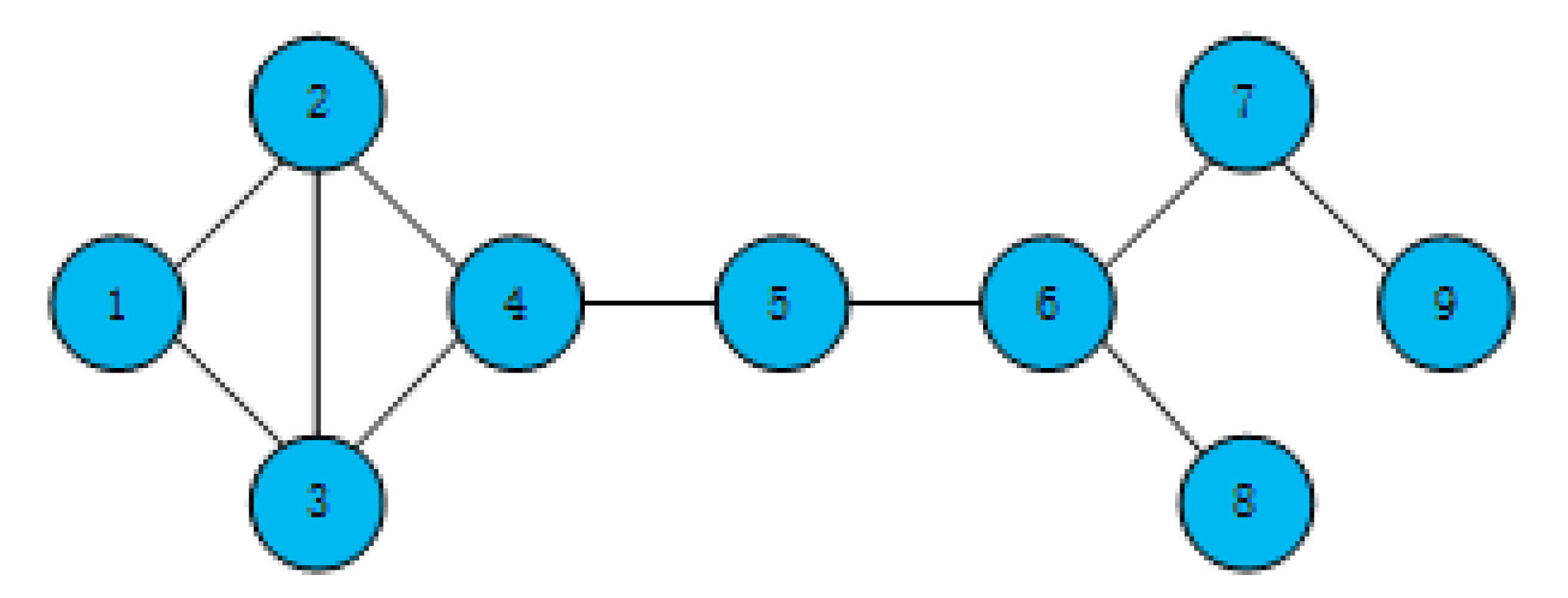
Take the toy network in Figure 1 as an example; the calculated H-indexes of nodes are shown in

Table 1. The H-index of each node in Figure 1.

Node	1	2	3	4	5	6	7	8	9
H-index	2	2	2	2	2	2	1	1	1

.

Algorithm 1: H-Index

Input: network G, node n Output: node’s H-index h nd = {}; h = 0; forvin G.neighbors(n) do   nd[v] = G.neighbors(v).length();   snd = sorted(nd.values(), descending);   for (i = 0; i < snd.length(); i++) do    h = i;    if snd[i] < i then     break; returnh;

2.2.3. SH-Index

Although the H-index can be applied to quickly calculate the influence of a node, the distinction of the node influence is very low, because the H-index only considers the neighboring nodes of a node but does not regard the node itself. In this paper, considering the node itself as well as its neighboring nodes, the SH-index of node $i$ (marked as $SH\left(i\right)$) is proposed, which is relevant to node’s H-index and its neighboring nodes, and it is defined as

$$SH\left(i\right)=\frac{H\left(i\right)\ast \left({\prod }_{j\in N\left(i\right)}H\left(j\right)\right)}{\left|N\left(i\right)\right|},$$

(3)

where $N\left(i\right)$ is the set of node $i$’s neighboring nodes, and $\left|N\left(i\right)\right|$ represents the degree of node $i$. The pseudo-code of calculating a node’s SH-index is shown as Algorithm 2.

Algorithm 2: SH-Index

Input: network G, node n Output: node’s SH-index sh sh = n.H-index(); N = G.neighbors(n).length(); forvin G.neighbors(n) do   sh *= v.H-index(); sh /= G.neighbors(n).length(); returnsh;

Likewise, take the toy network in Figure 1 for instance; the H-index of node 1 is 2, the list of its neighboring nodes is [2,3], and the H-index list of neighboring nodes is [2,2]. According to Equation (3), node 1 has an SH-index of 4. Similarly, the SH-index of all nodes is shown in the following

Table 2. The SH-index of each node in Figure 1.

Node	1	2	3	4	5	6	7	8	9
SH-index	4	5.3	5.3	5.3	4	1.3	1	2	1

.

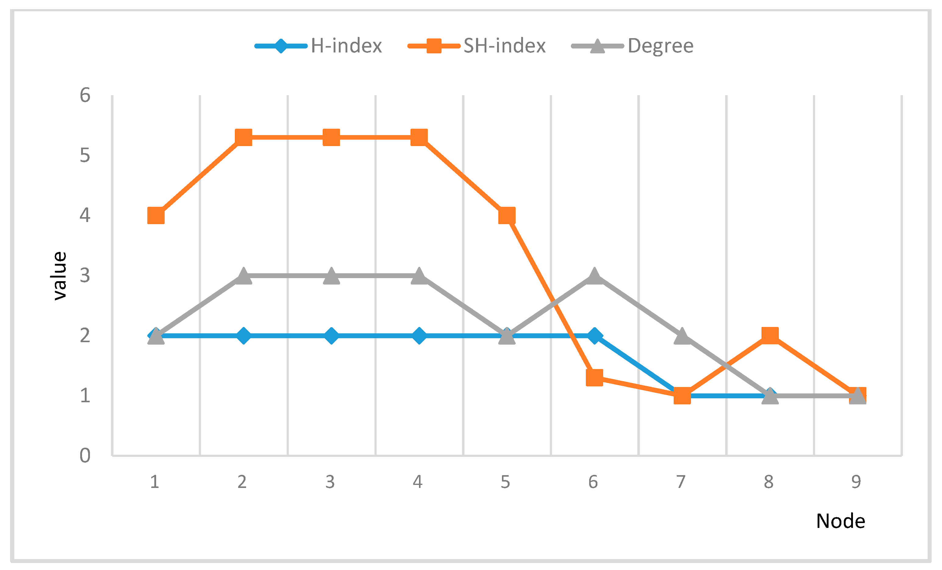
In the toy network in Figure 1, we can calculate the degree, H-index, and SH-index of each node, as shown in Figure 2.

Figure 2 shows that the SH-index can effectively solve the problem that the discrimination of nodes’ H-index is not obvious for nodes with similar degrees.

By employing the SH-index for calculation, the influence of the nodes can be apparently distinguished. Therefore, according to the value of the SH-index, the order of node updating in the LPA algorithm can be improved, and ultimately the stability of the LPA algorithm can be enhanced.

2.2.4. Update Rules of the SH-LPA Algorithm

The randomness of the LPA algorithm updating comes from the randomness of the order of node updating and the randomness of node labels updating, so in order to reduce its randomness, the SH-LPA algorithm changes its updating rules from the following two aspects:

First, the order of node updating. By calculating the SH-index of each node in a graph $G$, sort them in ascending order, and then update the node labels following the sorted order. Updating the labels in ascending order can make the algorithm converge as soon as possible, because a node with a small SH-index is first updated to a node label with a large SH-index in the neighbor, so that when a node with a large SH-index is updated, the label of the neighboring node is exactly its label and resulted without being updated; therefore, the algorithm can converge more quickly.

Second, the order of node labels updating. The node label is first updated according to Equation (1). When there are multiple choices, we update the current node’s label by selecting the node label with the maximal SH-index among the neighboring nodes of the current node rather than just randomly select one, as indicated by

$$l\left(i\right)=\underset{l}{argmax}{\sum }_{j\in N\left(i\right)}SH\left(j\right).$$

(4)

If there is still more than one result, then any one of them is randomly selected as the node label for updating.

2.3. Procedures of SH-LPA Algorithm

Given a network $G=\left(V,E\right)$, the process of the SH-LPA algorithm is as follows:

First step: calculate the SH-index of each node in $G$

(1) Traverse each node in $G$, calculate the H-index of each node in terms of Equation (2), then store each node and its H-index value as a dictionary node_h_index;

(2) Traverse each node in $G$ again, calculate the SH-index of each node according to Equation (3) and the node H-index of node_index, and store each node and the corresponding SH-index into a dictionary node_sh_index;

(3) Sort node_sh_index in ascending order.

Second step: updating the process of the SH-LPA algorithm

(1) Initialize each node in $G$ as a unique label;

(2) Obtain the SH-index list visit sequence of each node;

(3) Traverse each node in the visit sequence in turn and update the label of the node in terms of the update rules in Section 2.2.4;

(4) Repeat Step (3) until the label of each node reaches the maximum value of the neighboring node label or the algorithm iterates to the maximum number of times, and the algorithm terminates.

Third step: re-traverse each node in graph $G$, and then store them in the dictionary communities with the node label as the key and the node as the value, so that the nodes with the same label share the same key; that is, the community division is completed.

The pseudocode of the SH-LPA algorithm and method of calculating the SH-index are as shown in Algorithm 3.

Algorithm 3: SH-LPA

Input: a network G Output: community C initialize node’s label in G and calculate node’s SH-index;//according to Equation (3); visitSequence;//sorting node’s SH-index by ascending order; i = 0; whilei < Kor node’s label != neighbor’s maximum label do   i += 1;   for v in visitSequence do     label = G.node(v).label;     m = getMaxNeighborLabel(v);//according to Equation (1);     if m.length() > 1 then       L = getMaxNeighborSHIndex(v);//according to Equation (4);       if L.length() > 1 then         label = random.choice(L);       label = L; forninG.nodes do   l = n.label;   C[l].append(n); returnC;

2.4. Complexity Analysis

Given a network $G$, the number of nodes is $N$, and the average number of neighboring nodes of each node is $K$.

2.4.1. Space Complexity

For this network $G$, the space required to store each node in the network is $O\left(N\right)$; during the execution of the algorithm, initializing a unique label for each node requires space $O\left(N\right)$; the space required to store the result of calculating H-index is $O\left(N\right)$. According to the H-index of the node, the space required to store the SH-index is $O\left(N\right)$; when sorting the SH-index result sequence, the required space complexity is $O\left(logN\right)$ by the fast sorting algorithm. Therefore, the total space complexity of the algorithm is $O\left(4N+logN\right),$ which is simplified as $O\left(N+ logN\right)$.

2.4.2. Time Complexity

First, initialize a unique label for the node and traverse each node in the graph; the time complexity is $O\left(N\right)$. Then, calculate the H-index of each node and find the neighboring nodes of each node; the time complexity is $O\left(k\right)$, so the time complexity for finding the neighboring nodes of all nodes is $O\left(kN\right)$. The result of the calculated H-index is also stored as the data structure of the dictionary, and the SH-index of the node is calculated according to the H-index of the node. The time complexity of the H-index of the neighbor node of each node is $O\left(k\right)$, the time complexity of finding the H-index is $O\left(1\right)$, the total time complexity is $O\left(kN\right)$, and the data structure of the dictionary is stored. The SH-index sequence of the node is sorted in ascending order, and the time complexity is $O\left(NlogN\right)$. Then, the time complexity of the SH-LPA algorithm used in this part is $O\left(N+2kN+NlogN\right)$, which is approximate to $O\left(kN+NlogN\right)$.

Then, according to the ascending sequence of the SH-index, the process of the LPA algorithm is executed, and the time complexity is $O\left(N\right)$. Assuming that the algorithm converges after m iterations, the time complexity is $O\left(mN\right)$. Then, the total time complexity of the SH-LPA algorithm is $O\left(kN+mN+NlogN\right)$, which is simplified to $O\left(kN+NlogN\right)$. That is, the SH-LPA algorithm is still close to linear time complexity.

3. Community Detection Algorithm for Multilayer Networks (MSH-LPA)

3.1. Constructing the Model for Multilayer Networks

A multilayer network can be regarded as a combination of multiple single-layer networks, but with the same number of nodes in each layer, various edges between nodes in the different layers, and the possibility of isolated nodes. The nodes between any two layers are a one-to-one correspondence. Therefore, a multilayer network consisting of L layers can be represented as $G=\langle G^{\left(1\right)},G^{\left(2\right)},\dots ,G^{\left(l\right)}\rangle$, where $l\in L$ and $G^{\left(l\right)}=\left(V,E\right)$. At present, the main merging methods are as follows: Reference [28] defines a merged adjacency matrix based on a multilayer network. If in a layer or layers of a multilayer network, two nodes are connected by at least one edge, an edge exists between these two nodes in the matrix. This method is easy to understand but ignores the fact that the edges between the same nodes in different layers of a multilayer network represent different meanings. In addition, if community detection is performed using the merged adjacency matrix, the result may be inaccurate, because it does not well reflect the tightness between the multilayer network nodes. The authors in [29] proposed a method called Network Integration to integrate information by calculating the average interaction of nodes in a multilayer network. This method considers the fact that the interaction between the different layers of the network is different, but it treats each layer of the network as equivalent, which makes the network different from the actual situation. Strehl et al. [30] proposed Partition Integration, which first performs community detection at each layer and then constructs a structural similarity matrix for each layer. Within a multilayer network, if two nodes in each layer belong to the same community, then the similarity of these two nodes is 1; otherwise, it is 0. However, only 0 and 1 are insufficient to describe the similarity of each single-layer network because the similarity of the two nodes is different in each layer, but here, they are all set to 1. Some researchers consider the number of edges between two nodes in the process of merging, so that the number of edges is accumulated, and it is regarded as the weight of the edge after merging.

As we have known, in each layer, the meaning of the connected edges between two corresponding nodes in a multilayer network is different, such as the edge between two nodes in a layer representing a relative relationship, but in another level, the connection between the two corresponding nodes may represent a friend relationship, or it may also represent a business relationship, and so on. According to common sense, we know that the edges with a relationship of relatives and friends are more important than that of business, so the weight of the edges should be distinguished, and it is obviously not appropriate to simply accumulate the weights or the number of edges. The following describes the multilayer network merging method proposed in this paper.

In a complex network, the greater the similarity between two nodes, the more similar the two nodes tend to be, and naturally the closer the relationship of the two nodes will be. Therefore, the weight of the edge is obtained by calculating the similarity between two nodes of an edge. The larger the value of the similarity, the larger the weight of the edge will be. In this paper, the similarity is calculated using Jaccard similarity, which is formulated as

$$S_{a,b}=\frac{\left|A{{\displaystyle \cap }}^{\text{}}B\right|}{\left|A{{\displaystyle \cup }}^{\text{}}B\right|},$$

(5)

where $A$ represents the set of neighboring nodes of node $a$, and $B$ represents the set of neighboring nodes of node $b$.

In the process of calculating similarity, two nodes in a multilayer network have no connected edges at each layer, so the similarity is not calculated even if the similarity is high, because in the process of merging the network, if there is no edge in each layer, then there must be no connected edges after merging. Considering an edge that exists in one layer between two nodes but no edge in another layer between the two corresponding nodes, we define two different types of edges:

same_layer_edge: the edge that exists between the nodes in layer l of the multilayer network;

latent_edge: the edge that exists in layer l but does not exist in the other one or more layers.

Depending on the type of the edge, we define the weights of the edges of the merged network as follows:

$$w\left(a,b\right)=S_s\left(a,b\right)+S_l\left(a,b\right),$$

(6)

where $S_s\left(a,b\right)$ denotes the result by employing same_layer_edge, and $S_l\left(a,b\right)$ is the result by using latent_edge.

According to Equation (6), by looping through each layer of the multilayer network, the weights of all edges of the merged network can be calculated until a weighted network is ultimately obtained.

3.2. MSH-LPA Algorithm

After building the multilayer network model, we obtained a weighted network. The larger the sum of the weights of all the edges of a node, the greater the influence of the node will be. Therefore, based on the SH-LPA algorithm, the MSH-LPA algorithm considers the weight of the edge of the node. The influence of the node is calculated by the sum of the SH-index of the node and the weight of the node (indicated as the MSH-index), and the updating order of the nodes and labels of nodes in the network are determined in terms of the size of the MSH-index of the node.

3.2.1. SH-Index Processing

From the calculation of the weight of the merged network, the similarity between two nodes’ ranges can be concluded $\left[0, 1\right]$. Assuming that each layer of the L-layer network is kept the same, and the maximal similarity of the two corresponding nodes is employed, the weight of the merged network is in the range of $\alpha \times \left[0, L\right]$, $\alpha \in \left[-1,1\right]$, and therefore the weight ranges $\left[-L, L\right]$.

In this paper, the log function is employed to reduce the SH-index by a certain proportion, and a new SH-index (denoted as ($\acute{SH}$)) is obtained, which is formulated as

$$\acute{SH}\left(i\right)=\log (\mathrm{SH}\left(i\right)).$$

(7)

3.2.2. MSH-Index

After the normalization of the SH-index, the numerical ranges of the SH-index and the weight are approximately the same, so the weight and the $\acute{SH}$ index can be jointly used to evaluate the influence of the node, which is denoted as follows:

$$MSH\left(i\right)=\acute{SH}\left(i\right)+{\sum }_{j\in N\left(i\right)}\frac{w\left(i,j\right)}{\left|N\left(i\right)\right|},$$

(8)

where $N\left(i\right)$ is the set of neighboring nodes of $i$, and $\left|N\left(i\right)\right|$ represents the number of neighbors. The metric for evaluating $i$ is better because it considers the influence that comes from the neighbors of different layers more. $\acute{SH}\left(i\right)$ depicts the basic influence of node $i$ in a conventional graph model, which dominates the updating order in the improved label propagation algorithm (i.e., MSH-LPA). The influence of neighboring nodes from different layers are represented by $w\left(i,j\right)$ in the transformed weighted network, and it is divided by the degree of node $i$, so the influence is described as ${\displaystyle \sum }_{j\in N\left(i\right)}\frac{w\left(i,j\right)}{\left|N\left(i\right)\right|}$, which is mainly used to distinguish the nodes with the same SH-index. The experiments conducting on SH-LPA have proved that the algorithm is more stable than LPA, and we have fully utilized the layers information and made the nodes easier to distinguish, so the metric is better than the previous one, as the comparison in experiment illustrated.

3.2.3. Updating Rules of MSH-LPA

The MSH-index is proposed based on the SH-LPA algorithm, so the MSH-index determines the order of node updating and node label updating in the MSH-LPA algorithm.

First, update the order of nodes. Here, we follow the same process as the order of node updating for the SH-index in Section 2.2.4, except that we replace the SH-index with the MSH-index.

Second, update the order of labels. Here, we still follow the same process as the order of node labels updating for the SH-index in Section 2.2.4, except that we replace the SH-index with the MSH-index, which is formulated as

$$l\left(i\right)=\underset{l}{argmax}\sum _{j\in N\left(i\right)}MSH\left(j\right),$$

(9)

where $N\left(i\right)$ is the set of neighboring nodes of node $i$.

If there is still more than one maximal neighboring labels at this time, then one of them is randomly selected as the node label for updating.

The detailed implementation process is essentially in agreement with the SH-LPA algorithm, except that SH is replaced by MSH.

3.3. Complexity Analysis

For a merged network $MG$, the number of nodes is defined as $N$, the average degree of nodes is $k$, and the number of edges is $E$.

3.3.1. Space Complexity

For this merged network $MG$, the space required to save each node in the network is $O\left(N\right)$); the space required to store the weight of the edge is $O\left(E\right)$.

Algorithm initialization phase: Initialize a unique label for each node, in which the required space is $O\left(N\right)$. after calculating the node’s H-index, the result needs to be stored, and the required space is $O\left(N\right)$. According to the node’s H-index, the space required to store the result of the SH-index is $O\left(N\right)$; the space complexity required to calculate the $\acute{SH}$ index is $O\left(1\right)$; and the space complexity required to store the MSH-index is $O\left(N\right)$. When sorting the MSH-index result sequence, the required space complexity is $O\left(logN\right)$ by the fast sorting algorithm. Therefore, the subtotal space complexity of the algorithm is $\left(E + 5N+ logN\right)$, and it is approximated as $O\left(E + logN\right)$.

3.3.2. Time Complexity

Initializing the label of the node in the graph $MG$ requires traversing each node in the graph with a time complexity of $O\left(N\right)$.

Calculating the MSH-index of each node: (1) For the H-index of each node, the time complexity required to traverse the neighboring nodes of the node is $O\left(k\right)$, and the H-index calculation result of the node is stored as the data structure of the dictionary. So, the time complexity of $N$ nodes is $O\left(kN\right)$. (2) Then, we calculate the SH-index of the node according to the H-index of the node, and we also need to find the H-index of the neighboring node; here, the time complexity is $O\left(1\right)$, the time complexity of traversing the neighboring nodes is $O\left(k\right)$, and the time complexity for storing the SH-index as a dictionary data structure is $O\left(kN\right)$. (3) The data of the node’s SH-index is normalized to obtain the $\acute{SH}$-index, and the time complexity is $O\left(N\right)$. (4) When calculating the MSH-index of a node, it is necessary to know the weights of all the edges of the node, and still traverse the neighboring nodes of the node; here, the time complexity is $O\left(k\right)$, and the time complexity is $O\left(kN\right)$ for N nodes. (5) The time complexity of sorting the MSH-index sequence in ascending order is $O\left(NlogN\right)$. Then, the partial time complexity of the MSH-LPA algorithm is $O\left(N+3kN+NlogN\right)$, and it is approximated as $O\left(kN+NlogN\right)$.

The process of the LPA algorithm: Execute the LPA algorithm following the SH-index in ascending order, in which the time complexity is $O\left(N\right)$. Assuming that the algorithm converges after the algorithm iterates for $m$ times, the time complexity is $O\left(mN\right)$.

After analyzing the time complexity in the three main stages of the MSH-LPA algorithm, the total time complexity of the algorithm is $O\left(N+kN+NlogN+mN\right)$, which can be approximated as $O\left(N+NlogN\right)$.

4. Experimental Results and Analysis

In this chapter, the SH-LPA algorithm and the MSH-LPA algorithm are compared and analyzed with the LPA algorithm and CDMN algorithm that divides communities by calculating the influence of nodes [31], respectively. We set up the following experimental environment: processor Intel (R) Core (TM) i7-2600CPU@3.40GHz, Memory 8GB, Hard disk 930G, Operating System Windows10, Programming Language Python 3.7.

4.1. SH-LPA Algorithm

The following five network datasets were employed for this experiment. The evaluation index is modularity, and the higher the modularity, the better the experimental results.

4.1.1. Dolphin Network

The dolphin network is a network of dolphins that Lusseau et al. used for seven years to observe the exchanges between 62 dolphins in the Doubtful Sound Channel; the network comprised 62 nodes and 159 edges, in which the average node degree was 5.1290.

Experimenting on the dolphin network, the modularity changing trends of LPA, SH-LPA, GN, and SCAN that nodes are clustered according to the way they share neighbors are shown in Figure 3.

It can be seen from Figure 3 that the modularity of the LPA algorithm fluctuates when the number of iterations follows between 100 and 1000 because of the randomness of the LPA algorithm. The modularity of the improved SH_LPA is marked as an orange line and is relatively stable and even higher than LPA.

4.1.2. Email Network

The Enron email communication network (http://snap.stanford.edu/data/email-Enron.html) covers all the email communication within a dataset of around half a million emails. This data were originally made public, and posted to the web, by the Federal Energy Regulatory Commission during its investigation. This dataset is the largest connected subgraph, comprising 291 nodes and 3099 edges, in which the average node degree equals 21.2990.

Experimenting on the email network, the modularity changing trends of LPA, SH-LPA, GN, and SCAN are shown in Figure 4.

It can be concluded from Figure 4 that the modularity of the LPA algorithm fluctuates from 100 to 400 on account of the randomness of the LPA algorithm. The modularity of the improved SH_LPA, which is marked as a gray line, is comparatively stable and even higher than that of the LPA.

4.1.3. Chengdu Bus Route Network

The network of the Chengdu bus route (https://www.neusncp.com/api/view_dataset?dataset_id=163) comprises 1895 nodes and 3051 edges, in which the average node degree is 3.2760. The dataset of the transportation system in Chengdu, China was collected by our team members manually.

Experimenting on the Chengdu bus route network, the modularity changing trends of LPA, SH-LPA, GN, and SCAN are shown in Figure 5.

It can be seen from Figure 5 that the modularity of SH_LPA is reasonably stable and even higher than that of the LPA algorithm.

4.1.4. DBLP Collaboration Network

The network of the DBLP (Digital Bibliography & Library Project) collaboration (http://snap.stanford.edu/data/com-DBLP.html) comprises 3911 nodes and 6244 edges, in which the average node degree is 3.1930. Since the GN algorithm does not run out of results in the same time, we use the largest connection subgraph of the author’s network.

Experimenting on the authors’ network, the modularity changing trends of LPA, SH-LPA, GN, and SCAN are shown in Figure 6.

It can be seen from Figure 6 that the modularity of the SH_LPA is relatively stable and even higher than that of the LPA algorithm.

4.1.5. Network of Scientists Cooperation

The original dataset (http://www.umich.edu/~mejn/centrality) contains 1589 nodes and 2742 edges. This dataset is the largest connected subgraph, which contains 379 nodes and 914 edges, and the average node degree is 4.8232, mainly representing co-authorships between 379 scientists whose research centers on the properties of networks of one kind or another.

Experimenting on the scientists’ cooperation network, the modularity changing trends of LPA, SH-LPA, GN, and SCAN are shown in Figure 7.

It can be seen from Figure 7 that the modularity of the LPA algorithm fluctuates from 100 to 300. This is because of the randomness of the LPA algorithm. The improved SH_LPA is relatively more stable than that of the LPA and simultaneously holds a higher modularity.

It can be seen from the above five figures that line charts of the SH-LPA algorithm close to a straight line and the line charts of the LPA algorithm are more complicated in the dolphin network, email network, Chengdu bus route network, authors’ network of DBLP, and the scientists’ cooperation network. In short, the variation range of modularity $Q$ in the SH-LPA algorithm is smaller than that in the LPA algorithm, and the SH-LPA algorithm is smoother than the LPA algorithm. Therefore, the experimental results and analysis from the above five experimental datasets can sufficiently prove that the SH-LPA algorithm proposed in this paper improves the stability of the LPA algorithm.

According to the modularity results of the above five experimental SH-LPA, LPA, GN, and SCAN algorithms, the average modularity is shown in Figure 8.

It can be seen from Figure 8 that the average modularity of the SH-LPA algorithm in this paper is comparatively higher than the LPA and the SCAN algorithm, and it is even slightly higher than the GN algorithm accounting to the average modularity. It can be concluded that the SH-LPA algorithm outperforms the LPA algorithm in modularity comparison. It proves that the proposed SH-LPA algorithm improves the stability as well as the accuracy.

4.2. MSH-LPA Algorithm

The experimental results and analysis are based on modularity. The following four datasets are employed as the experimental multilayer networks.

4.2.1. Students’ Cooperation Social Network (SCSN)

The dataset [31] is a social network built on the homework of 185 students in two different majors at Ben-Gurion University to complete the compulsory course of computer network security. The network has a total of 360 edges with three types—‘time’, ‘computer’ and ‘partner’; here, ‘time’ denotes that two students link with each other if they submit assignments within the same period, ‘computer’ means students submit the assignment on the same computer, and ‘partner’ indicates that students complete the assignment together.

4.2.2. Enron’s Mail Network

The network [32] consists of 151 nodes and 266 edges, and there are two types of edges: mail exchanges between supervisors and subordinates and mail exchanges between colleagues.

4.2.3. Indonesian Terrorist Network

The Noordin top terrorism network [33] was drawn primarily from the "Terrorism in Indonesia: Noordin’s Network", which is a publication of the International Crisis Group (2006) and includes relational data on the 79 individuals listed in Appendix C of that publication. The data were initially coded by Naval Postgraduate School students as part of the course “Tracking and Disrupting Dark Networks” under the direction of Professor Sean Everton, Co-Director of the Core Lab, and Professor Nancy Roberts. CORE Lab Research Assistant Daniel Cunningham reviewed and cleaned all the coding made by students. This paper extracts four types of edges from the relationship of the 79 people in the network dataset, namely, ‘classmates’ (175 edges of classmate relationship), ‘training’ (186 edges of training relationship), ‘communication’ (200 edges of communication), and ‘business’ (30 edges of business dealings).

4.2.4. 9/11 Terrorist Dataset

The 9/11 terrorist dataset [34] contains 62 nodes and 153 edges. In the real world, most terrorists of the dataset started as friends, colleagues, or relatives; they were drawn closer by bonds of friendship, loyalty, solidarity, and trust, and rewarded by a powerful sense of belonging and collective identity. The data are supplied in an edge-list file, in which two numbers signify the strength of tie (5 = strong tie, 1 = weak tie) and the level to which the tie has been verified (1 = confirmed close contact, 2 = various recorded interactions, 3 = potential or planned or unconfirmed interactions).

The modularity obtained by the MSH-LPA algorithm and CDMN algorithm on the above four network datasets is shown in Figure 9.

As shown in Figure 9, the MSH-LPA algorithm obtains higher modularity conducting on the four real-world datasets than the CDMN algorithm.

5. Conclusions

By analyzing the instability of the label propagation algorithm (LPA), it is concluded that the randomness of node and node labels updating in the LPA algorithm can be changed by calculating the centrality of the node, and then improving the stability of the LPA algorithm. The deficiency of the H-index directly applied to the LPA algorithm is described in detail, and the SH-index is proposed. Based on the SH-index, the SH-LPA algorithm is presented. The stability of the algorithm is verified by experiments, as is the time complexity of the algorithm is $O\left(kN+NlogN\right)$, which is close to linear time complexity.

In order to solve the problem that much network information may be lost when merging a multilayer network into a single-layer network, the similarity of the nodes is employed to determine the weight of the edge of the merged network, and the multilayer network is merged into a weighted single-layer network, in which the SH-index and the weight of the node jointly determine the order of node and node labels updating. Here, we propose a more accurate MSH-LPA algorithm.

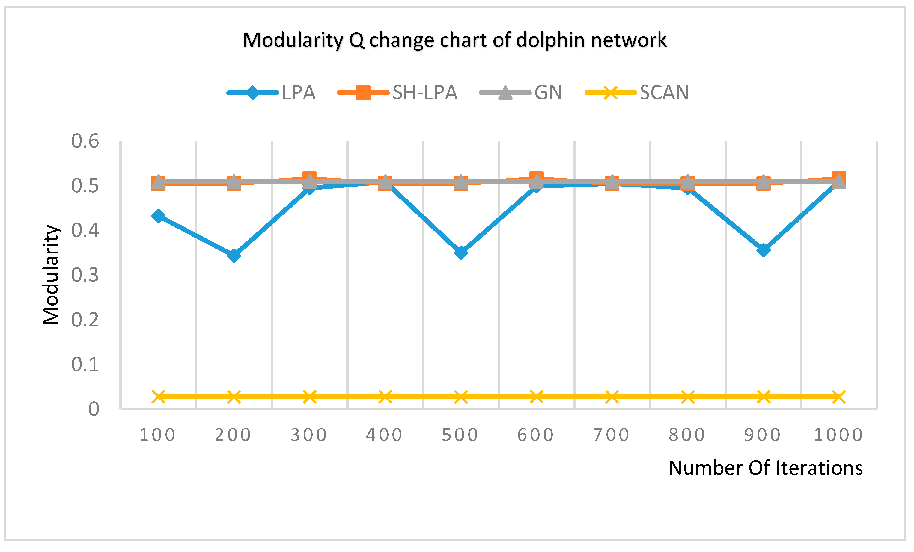
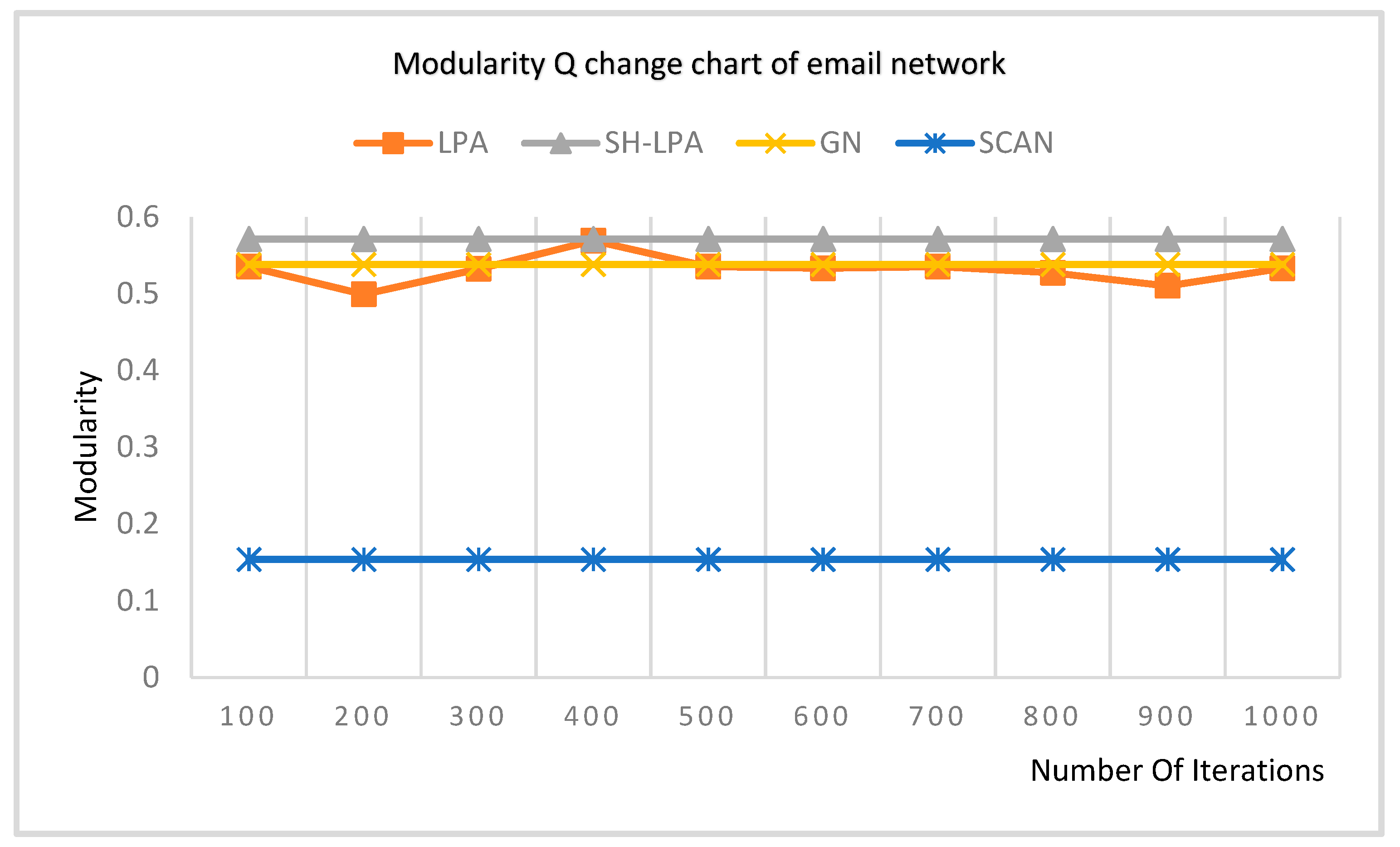
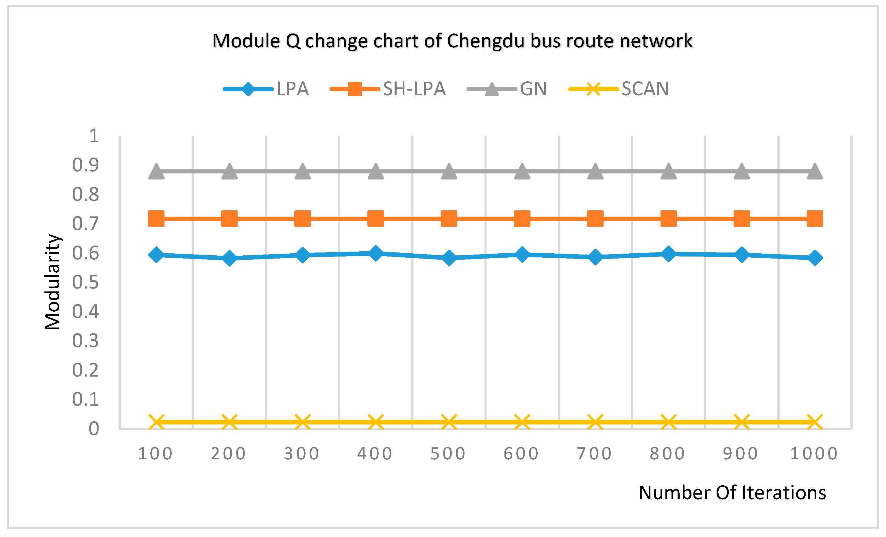
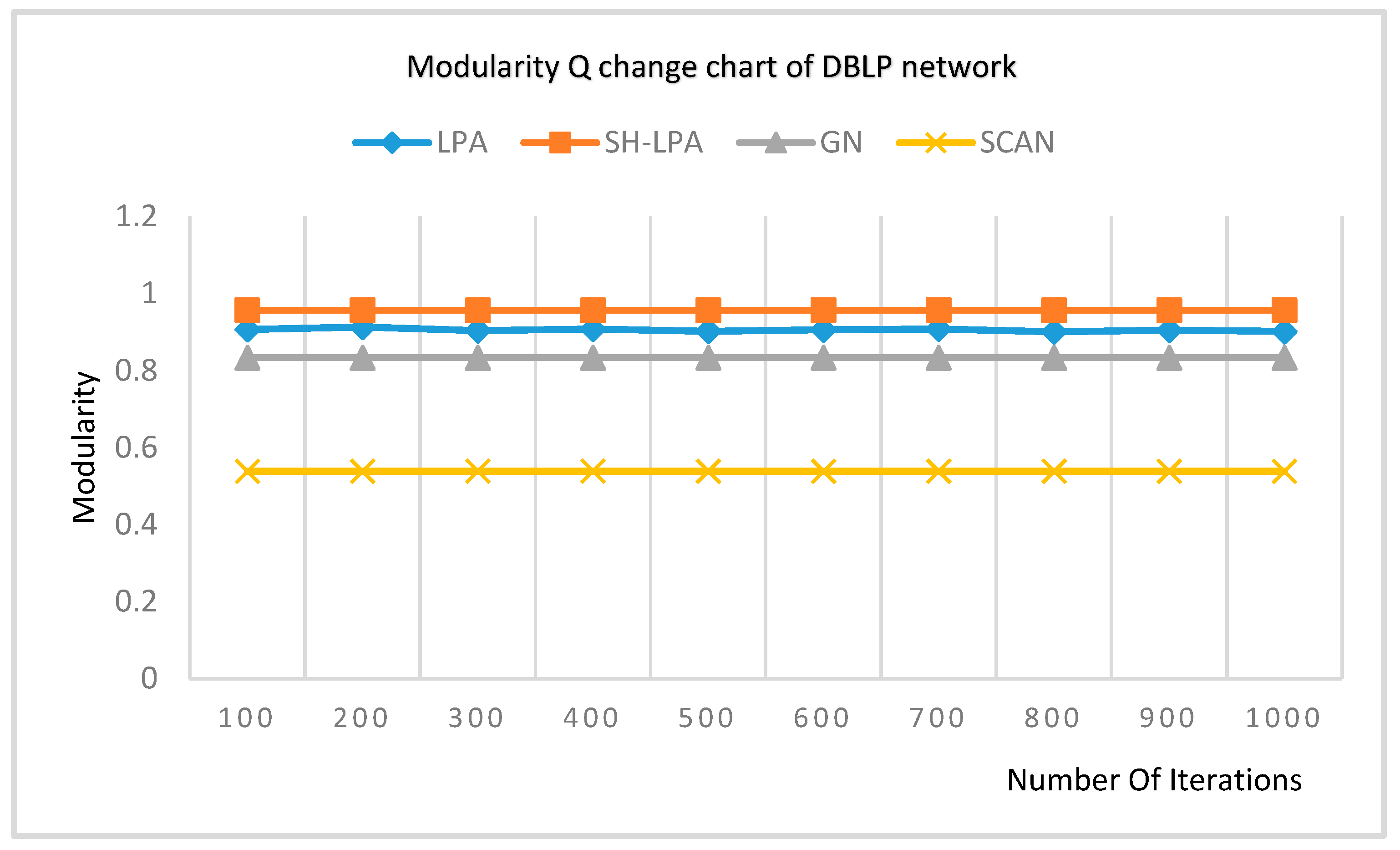
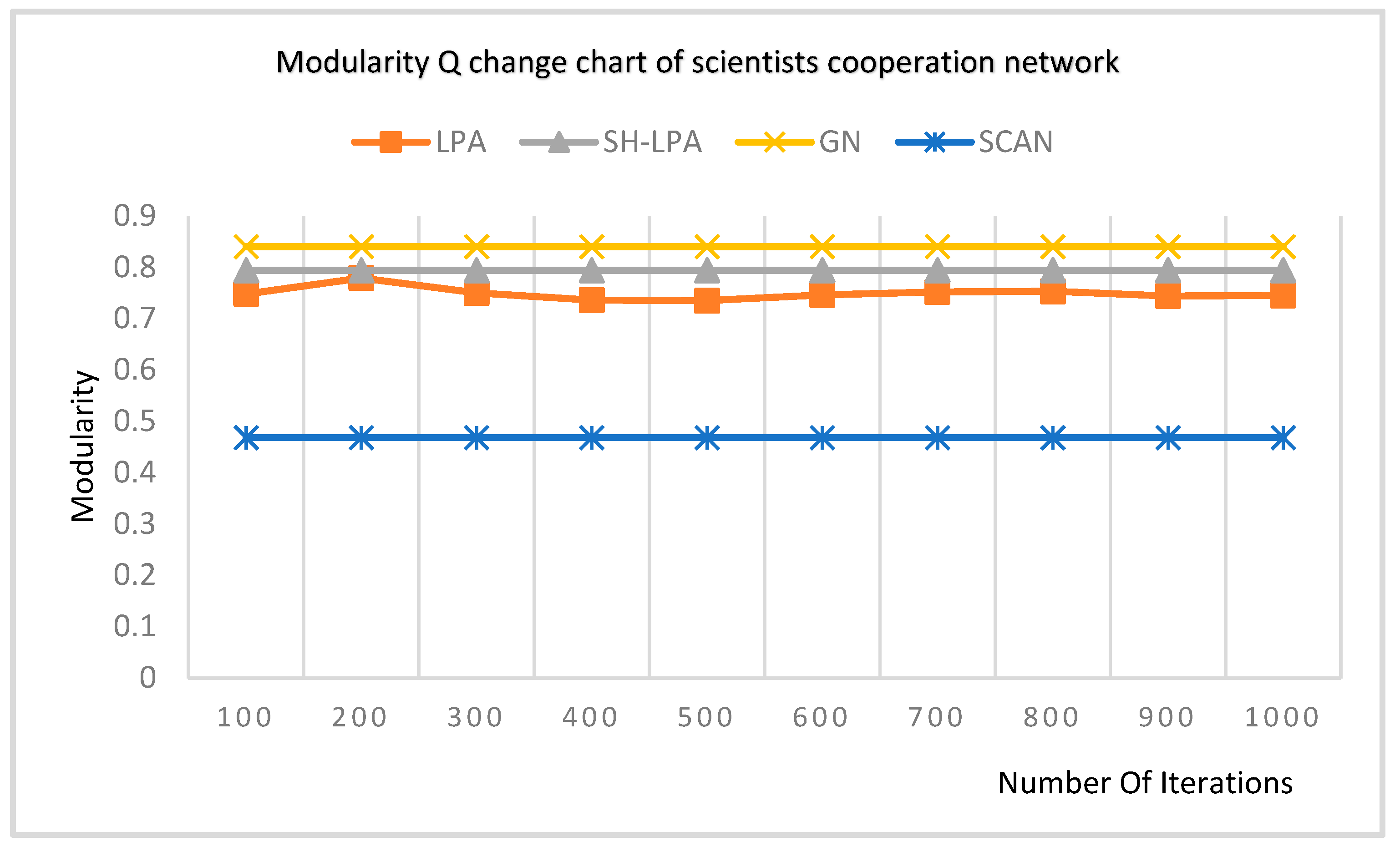
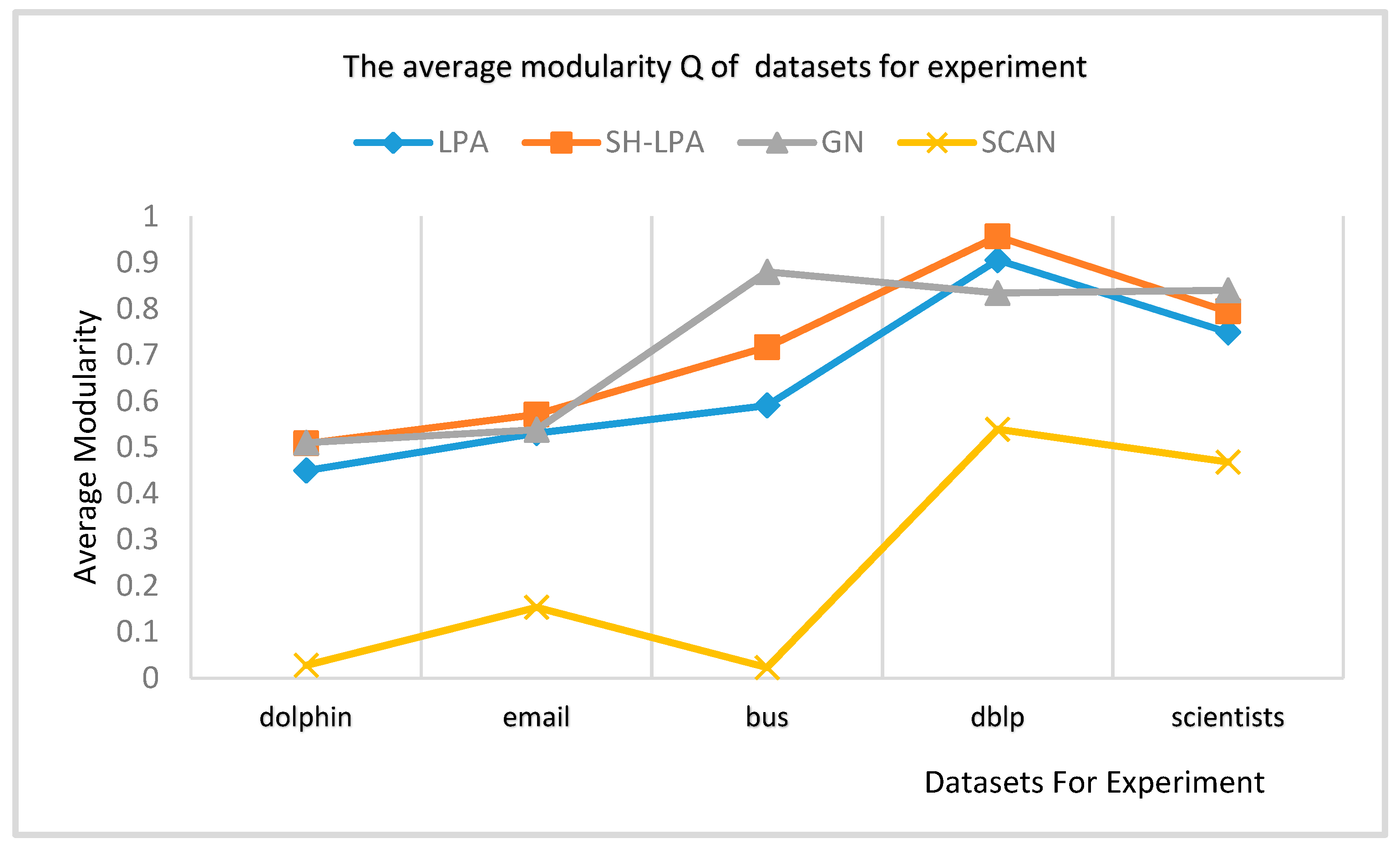
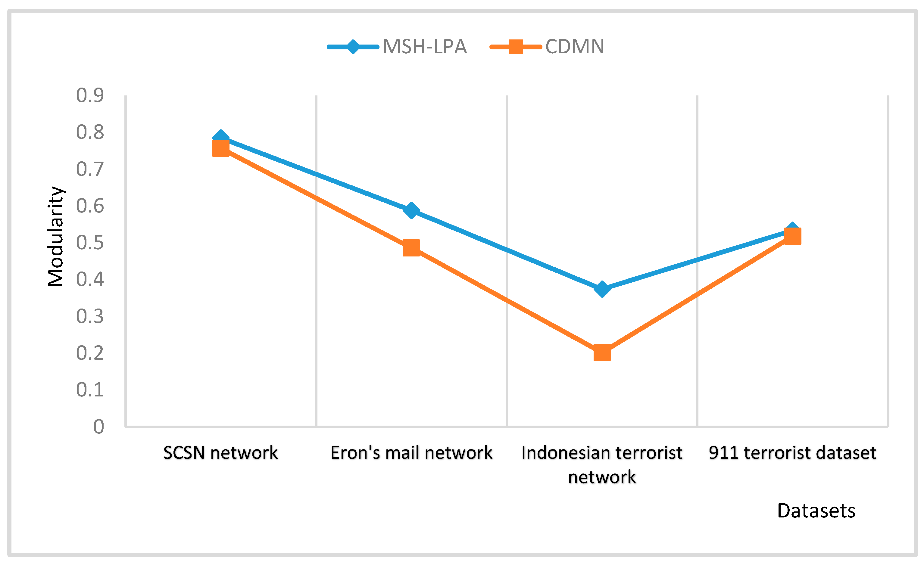
In order to verify the superiority of the SH-LPA algorithm and the MSH-LPA algorithm, the experimental results on five datasets show that the SH-LPA algorithm improves the stability of the LPA algorithm. Compared with the CDMN algorithm on the four multilayer network datasets, it is proved that the MSH-LPA algorithm proposed in this paper achieves larger modularity than the CDMN algorithm, which indicates its higher accuracy.