1. Introduction
Often when solving problems, it becomes necessary to assess the similarity of objects. In some cases, this problem is solved by correlation analysis methods. Moreover, methods of cluster analysis have become widespread, dividing a set of objects according to the values of their attributes into groups. The most famous and simple methods of cluster analysis use the following approach: objects are combined into clusters based on the values of the distances between them, and the merging process is regulated by the selected method, i.e., when solving the problem of cluster analysis, it is necessary to choose a metric and a partitioning method. Different partitioning methods and metrics are better suited for different types of objects and different clustering goals. In particular, for clustering time series, separate types of metrics are required that consider the peculiarities of such data: the presence of a dependence on time, which is expressed in the dynamics of the series, and the complexity of the structure of the series, which is measured by various indices and coefficients. In recent decades, for particular problems, a large number of metrics have been proposed, which either consider a priori assumptions about the form of a model that well describe the dynamics of the series, or measure the distance between objects based on various characteristics of the series. Thus, there is no generally accepted metric for clustering time series; for each task, it is necessary to select an individual approach.
One of the directions in which the analysis of the similarity of time series can be applied is the sphere of speech technologies. A lot of research in this area is aimed at analyzing the parameters of the speech signal. One of these parameters is the fundamental frequency (F0). Knowing the F0 of a signal at a particular point in time is important in many areas of speech technology.
Determining the features in the fundamental frequency of a speech signal is an important task in the field of studying the features of the language. Some languages and accents are characterized by the appearance of an ascending or descending tone, which in its characteristics may be similar to vocal performance. The works of [
1,
2] consider the possibility of using the detection of an ascending–descending tone in speech as a marker for deciding whether a speaker has a Welsh accent. The authors evaluated intonation based on whether the voice was raised or lowered. The resulting F
0 spread was obtained in the range from 169 to 358 Hz. The study of [
3] raised the issue of determining the characteristics in the speech of young people. Based on the assessment of the F
0 of the recordings of speech signals, it was determined that intentional stretching of vowels is characteristic of young people. The authors of works [
4,
5,
6] conducted a study of the pitch-melodic parameter of speech, namely the influence of age-related changes on the rhythmic characteristics of the language. It was determined that with an increase in the speaker’s age, a decrease in the maximum and minimum values of the F
0 is manifested. One of the features of [
7] is the determination of the emotional state of the speaker based on the identification of the characteristics of the melody form in speech. The author drew attention to such characteristics as direction, character and range of tone movement. In this study, the values used in the study of musical melodies were used to measure the F
0. This made it possible to visually represent the features of changes in the speaker’s speech when emotions or intentions are displayed. A similar task was posed in [
8], where, based on the change in the difference in the acoustic values of the average and maximum frequency of a phrase, the evaluativeness in the speech of reporters was determined in order to convey the atmosphere of what was happening.
In addition, in the direction related to the identification of speakers, the F
0 of the speech signal also plays a role. In addition to formants reflecting the individual characteristics of a person, speaker identification systems also analyze the fundamental frequency of the signal under study. This is confirmed by the fact that the determination of the basic frequency of the speech signal, considering the peculiarities of speech formation and speech perception associated with human anatomy and physiology, is extremely important not only in studies on user identification [
9,
10,
11], but also in the field of rehabilitation for cancer patients after resection of the larynx [
12,
13]. The further choice of material for the study of the metric is due to the fact that it is easier to determine the reference frequencies when analyzing vocal performance than when studying speech.
Singing can be thought of as a special form of speech that is created in the same way, but there is additional control to create the musical aspect. The natural melody of speech (prosody) differs in different languages and determines the pitch contour, volume variation, rhythm and tempo of emotional expression. In singing, the pitch, volume and timbre are primarily determined by the composition due to the fact that to match the duration of the note, the vowels sound longer than usual. Speech vowels are characterized by special formant positions. In singing, the position of the formant can be radically altered by changing the length and shape of the vocal tract and the position of the articulators. A review of studies on music processing has shown that from the point of view of signal processing, a melody can be represented by sequences of F0 determined at the moments of sounding, that is, in areas where the instrument that creates the melody is active. This allows us to consider the study of the dynamics of the parameters of a speech signal as a time series.
The review of articles in the field of application of feedback from software for teaching singing showed that this topic is relevant. These studies provide different approaches to providing feedback to a singer based on the melody performed by them. Some of the more popular approaches include spectrogram displays, piano keyboards and frequency graphs [
14,
15,
16,
17]. Among other possibilities, the study of [
16] provides an additional opportunity provided by teaching with a software tool. The program can accumulate the results of the student, which can later be viewed and used to evaluate the changes in development that have occurred. This can have a positive effect on student motivation. Since the provided result is an assessment of physiological parameters (fundamental frequency), in further work, we will call this biofeedback [
18]. However, most of the works concentrate on the teaching method without giving detailed information about the quality of vocal performance processing. The algorithms used in the programs do not allow calculating the value of the fundamental frequency in a vocal performance with high accuracy due to the presence of a high percentage of gross errors in them or are limited by a narrow spectrum of covered frequencies.
The purpose of this research is to test the applicability of the metric of highlighting the synchronicity of time series for assessing the type of vocal performance with a sharp change in the fundamental frequencies. Previous research has concluded that the program complex for vocal recognition is able to identify notes with smooth frequency changes. A detailed description of the applied algorithm for identifying notes in vocal performance and the obtained test results will be published as part of a further study. As a result, vibrato and glissando singing styles were perceived as noise. Thus, the task of identifying these segments appeared.
In this issue, the value of the fundamental frequency is used as estimated information at the recognition of music sung by a speaker. This information is sufficient for identifying notes at each estimated moment in accordance with music theory. Further stages of note recognition include segmentation, taking into account the minimum sound duration and filtering out noise. Speaker identification is not a purpose of this study. Moreover, one of the tasks of the system development is maximizing the objectivity of the evaluation. The recorded note is determined by the fundamental frequency. Accordingly, the individual characteristics of the singer determined by their articulators do not matter for note identification. With further research of adjacent directions associated with more stringent requirements for the set of parameters, it is possible to expand the processed dataset.
Accordingly, the data analysis method should enable determining the type of singing based on the values of the fundamental frequencies in the investigated period of time. The developed software package is aimed at helping the user in individual singing lessons. Biofeedback provided by the program should tell the speaker if they sang the note incorrectly. In this matter, the promptness of the assessment is important. Accordingly, the processing of singing should be done in real time or for a comparable duration. Thus, the less information needs to be processed to get an estimate of the sung melody, the better. This method should not require large numbers of computations and has to be easy to implement.
Otherwise, real-time signal processing would be unattainable. In addition, the system should not depend on the speaker. The use of neural networks will require training the system on examples of singing with a change in the values of the frequencies of the main tone when playing a single note. Due to the fact that the system is being developed to teach speakers how to sing correctly, it is incorrect to set up the system based on the speaker’s initial exercises. There is a possibility that the system will evaluate the user non-objectively, since conclusions about the correct performance will be based on the speaker’s unformed ear for music.
2. Overview of Similarity Analysis Methods
Throughout history, humans have sought and accumulated knowledge about the world around them. Based on the knowledge gained, people ordered objects in accordance with their similarity. Often, such a grouping was essential for survival, for example, the division of plants into edible and inedible, animals based on danger and so on. This process of grouping objects by a person on some grounds is called classification.
A preliminary task for grouping is to determine the degree of similarity of objects by a particular attribute (or a set of attributes). In particular, the study of the degree of similarity of large amounts of data is a popular problem at the intersection of mathematics and climatology. The presence of such a similarity was considered, in particular, in [
19]. The author described the presence of similarities in the dynamics of the magma column shift in Iceland and the Hawaiian Islands and investigated the influence of these shifts on other factors: temperature, continental climate, amount of atmospheric dust, etc. The so far popular task of studying the influence of solar activity on temperature and pressure was considered in the study of [
20]. A large amount of values was investigated when determining the similarity of the behavior of atmospheric pressure at different stations in [
21].
In modern geophysics and climatology, determining the presence of similarity between different data is an important problem. In the books [
22,
23], many problems are considered, one way or another related to the problem of similarity. For example, in [
24,
25,
26], the determination of similarity is necessary to construct a function of the dependence of the maximum density of the annual ring on the total ozone content (TOC) in the atmosphere and for further reconstruction of unknown TOC values from this function. This task of the so-called bioindication is very important, since the series of ring densities are very long, while the TOC values have been measured only since 1927, and it is still impossible to carry out a correct analysis for them.
With the development of science, classification has also developed as one of its fundamental elements. However, until the last century, this process was based, first of all, on the natural capabilities of a person to recognize patterns and group objects. The 20th century is characterized by a sharp increase in scientific knowledge. Effective analysis of information becomes almost impossible for a person due to its volume and complexity and requires new approaches. Under these conditions, the automation of various areas of human activity through the introduction of computer technology has also affected the classification process. This is based on the idea of using mathematical methods to group objects in the real world. It is necessary to conduct research on methods for determining the similarity of objects.
Some of the simplest and most well-known methods for assessing the similarity of time series are correlation analysis methods. For the first time, the term correlation was introduced into scientific circulation by the French paleontologist Georges Cuvier in the 18th century. He deduced the principle of correlation of parts and organs of living beings, with the help of which it is possible to restore the appearance of a fossil animal, having only a part of its remains at disposal. He introduced the principle of correlation between parts and organs of animals. The principle of correlation helps to restore the appearance of an organism from the skull, bones, etc., found in excavations. The appearance of the entire animal and its place in the system can be assumed as follows: if the skull is with horns, then it was a herbivore, and its limbs had hooves; if the paw is with claws, then it is a predatory animal without horns, but with large fangs.
German psychiatrist G.T. Fechner (1801–1887) proposed a measure of the tightness of communication in the form of the ratio of the difference in the number of pairs of coinciding and non-coinciding pairs of signs to the sum of these numbers:
where
is the number of pairs in which the signs of deviations of values from their means coincide, and
is the number of pairs in which the signs of deviations of values from their means do not coincide.
The Fechner coefficient is a rather rough indicator of the tightness of communication, which does not consider the magnitude of deviations of features from the mean values, but it can serve as a certain guideline in assessing the intensity of communication.
One of the most popular correlation indicators is Spearman’s coefficient, calculated by the formula
where
and
are values of two time series of the same length.
When assessing the degree of similarity by calculating the correlation coefficients, a serious inaccuracy is possible, since the correlation coefficient shows the presence of a linear relationship between the data, while the relationship may not be linear or there will be partial similarity of objects.
In econometric problems, such kind of similarity of time series as cointegration is considered. Cointegration [
27] refers to a cause-and-effect relationship in the levels of two (or more) time series, which is expressed in the coincidence or opposite direction of their tendencies and random fluctuations. According to this theory, cointegration exists between two time series if the linear combination of the time series is a stationary time series (i.e., a series containing only a random component and having constant variance over a long period of time).
Additionally, such an approach to assessing the similarity of data as cluster analysis has received great development. The beginning of the development of cluster analysis dates back to the first half of the 20th century. A detailed description of cluster analysis is given in the book [
28]. Cluster analysis has several advantages over other methods of data classification. First of all, this is due to the fact that it allows you to split objects not one by one, but by a whole set of features. Moreover, the influence of each of the parameters can be rather simply strengthened or weakened by introducing the corresponding coefficients into the mathematical formulas. In addition, cluster analysis does not impose restrictions on the type of objects to be grouped and allows considering a variety of initial data of almost arbitrary nature. Another feature of clustering is that many algorithms are able to independently determine the number of clusters into which the data should be split, as well as highlighting the characteristics of these clusters without human intervention, only using the algorithm involved.
The great advantage of cluster analysis is that it allows you to split objects not by one parameter, but by a number of features. In addition, cluster analysis does not impose any restrictions on the type of objects under consideration, and allows considering a variety of initial data of almost arbitrary nature.
On the other hand, one of the key problems of cluster analysis is determining the number of clusters. Some methods require a priori determination of clusters, while in others, their number is determined in the process of agglomeration or division of a set of existing objects. One of the most frequently used methods for determining the number of clusters is the application of the “scree test”. The process of grouping objects in hierarchical cluster analysis corresponds to a gradual decrease in the average distance between clusters with an increase in the number of clusters. At the stage where this measure of distance stops decreasing abruptly, the process of partitioning into clusters must be stopped, since otherwise the partitioning of clusters is unnecessary. The optimal number is considered to be the number of clusters equal to the difference between the number of observations and the number of steps, after which the coefficient decreases smoothly.
Time series clustering methods are divided into two groups:
- (1)
Methods based on estimating the complexity of a time series;
- (2)
Methods based on model assumptions.
The methods of the first group are considered in the works of D. Sankoff and J. Kruskal [
29], D. J. Berndt and J. Clifford [
30], T. Oates, L. Firoiu and P.R. Cohen, E.A. Maharaj, M. Corduas and D. Piccolo, Chouakria A. Douzal, and PN Nagabhushan [
31]—these works propose an algorithm for dynamic-scale transformation, including using the theory of hidden Markov processes, using autocorrelation coefficients, spectral characteristics, wavelet coefficients and the adjustable difference index. In the studies of K.Y. Staroverov and V.M. Bure [
32,
33], they solve the narrower problem of clustering short time series. It is also possible to single out the method of identifying structures described in the works of S.G. Kataev [
34], which is applicable in various problems, including clustering of time series. Among the methods of the second group, the transition to autoregression coefficients is mainly considered as to the features—in particular, in [
35] for classification, in addition to autoregressive coefficients, the characteristics of a series are used—mean value, variance, etc. In [
36], the clustering after transformation and smoothing (CATS) approach is presented, in which it is proposed to construct approximating functions for the compared time series (transformation) before clustering, where the resulting curves are additionally smoothed (smoothing) and then the set of coefficients obtained are used as clustering objects. It is stated further that any clustering method can be applied; the k-means method is used in the work itself.
At the Institute for Monitoring Climatic and Ecological Systems of the Siberian Branch of the Russian Academy of Sciences in the laboratory of bioinformation technologies under the leadership of V.A. Tartakovsky, an approach to assessing the similarity of time series was developed considering the hypothesis of synchrony factors. The results are presented in the works of [
37,
38]. It is believed that the external forcing effect synchronizes natural and climatic processes and manifests itself in the similarity of their essential features. The essence of the approach is that orthogonal components of processes are introduced, which differ in the coincidence and non-coincidence of essential features, orthogonal expansion of the series under study is performed, similar to the principle of trigonometric Fourier transform, and then the correlation coefficient is calculated for the obtained components. If the correlation coefficient is high, the presence of synchronicity in the dynamics of the series is recognized. This method allows one to examine series of different lengths for synchronous behavior.
The concept of synchronicity of time series is also used in this study. We will call time series synchronous if the dynamics of their development are similar. Then, we can consider the problem of assessing the similarity of time series as an assessment of the degree of synchronicity of the series, that is, the synchronicity of the dynamics of time series is a special case of their similarity.
The review of articles has shown that standard classification methods are not suitable for solving this problem. To apply clustering methods, there should be several speakers, while in our task, the singing of one performer is studied, represented by one time series. For classification, it is necessary to preset the characteristics of the vibrato or glissando class, which at this stage of the study is not possible due to the lack of necessary information about the general laws of singing with such effects for any performer. Using Gaussian mixture model (GMM) also involves handling multiple speakers. This parametric probability density function is characterized by a feature data vector with the characteristics of the weights of these features. Accordingly, this approach is not suitable for this study. This is due to the fact that the work of the software package is not aimed at identifying the speaker from several options, but only the value of the fundamental frequency is used in the assessment.
3. Synchronicity Extraction Method
The novelty of the proposed method lies in the possibility of adjusting the parameters when assessing the similarity. Earlier, the software package implemented the ability to independently regulate the system’s requirements for the purity of the note performance. By default, each note is assigned a sound band with boundaries, determined from data from music theory. In this case, the lower boundary of each note starts from the last value that was not included in the previous note’s band. If desired, on the part of the speaker, it is possible to increase the system’s requirements for the quality of performance. This will narrow the boundaries for each note. As a result, the boundary frequencies between the notes will be perceived by the system as noise. This idea can be applied to assess the similarity of multiple time series. In contrast to traditional metrics, the proposed method presents the degree of similarity of time series as a percentage, which is convenient for a qualitative interpretation of the degree of closeness. The requirement for the rigor of the system in assessing similarity can be adjusted taking into account E, which allows increasing (or decreasing, if necessary) the complexity in the learning process.
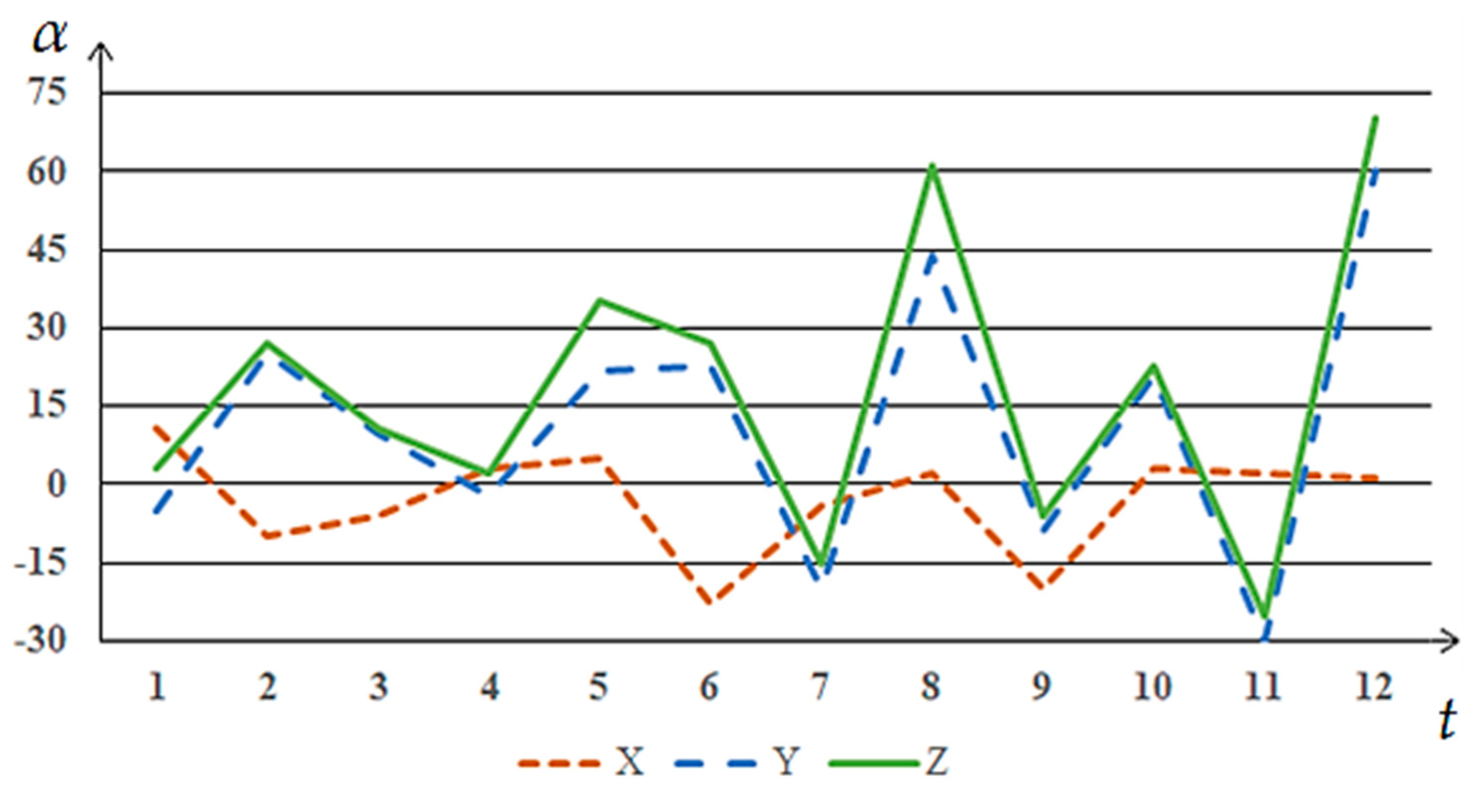
The synchronicity of the dynamics of time series is a rather subjective concept, which follows from the ambiguity of solutions to the problem of assessing the similarity of time series—there is no single indicator of either the degree of similarity of the series or the degree of their synchronicity. The concept of synchronicity can be best illustrated with graphs. Let there be given three time series X, Y and Z. Series X and Y have synchronous dynamics, and the behavior of series Y and Z is different.
Figure 1 shows their comparative graphs with synchronous and non-synchronous dynamics.
To simplify the understanding of the concept of synchronicity, we will assume that this graph shows the dependence of a certain value of alpha on time. The timeline in this example is split into 12 units representing months. The ordinate is the alpha value that changes over time. This value may have positive or negative values. The behavior of a quantity is determined by the research subject. In the presented study, the ordinate will be the fundamental frequency values, measured in Hz, and the abscissa will be the time scale in seconds. Each second of the processed audio recording contains 44,000 values. This number of values per second is determined by the sampling rate of the audio recordings made. The choice of the fundamental frequencies as the object of research is determined by the results of the previous research stages.
One of the most famous models of the time series
assumes its representation as the sum of two quantities:
where
is a deterministic component, which includes the entire pattern of the formation of the dynamics of a series under the influence of time, and
is a random component that describes all deviations caused by the influence of other factors.
Since in defining synchronicity the emphasis is placed on the dynamics of the development of the series, we will investigate only the deterministic component. Further, since the deterministic component can be described by some selected approximation function, we will consider the transition from assessing the similarity of the values of the series themselves to comparing the coefficients or values of the approximating function.
Consider the formal statement of the problem of assessing the degree of synchronicity. Let there be given two time series
. Suppose that the dynamics of series
and
are described, respectively, by the approximating functions
and
of the form
where
are some elementary functions,
, and
are coefficients,
.
Then, we can go from studying the similarity of time series
and
to studying the similarity of functions
and
and give a definition of the similarity metric of the time series. According to this, we call the synchronicity extraction metric the quantity.
where
is the indicator function defined as follows:
,where
is some condition that may or may not be hold, and then the indicator function argument is set to true or false.
Thus, to assess the degree of synchronicity of the dynamics of time series, the number of coefficients that differ by an amount less than a given critical value is calculated—in the framework of this study, we will call such coefficients “equal”. Since the distance is calculated using coefficients, it is necessary to consider the difference in the order of values and the contribution to the total value of the function of the corresponding components. If considering the contribution of the components requires additional information and features of calculating the metric, then the differences in values can be reduced by converting to a single scale using normalization by the formula
where
is the normalized value of the
-th coefficient in the approximating function for the
-th series,
;
is the number of coefficients;
is the original
-th coefficient in the function for the
-th series;
is the sample mean value of the
-th coefficient for the functions of all considered series; and
is the sample standard deviation of the
-th coefficient for the functions of all considered series.
Then, the value can be regarded as the proportion of the variances of the coefficients of the compared series or the variance of the values of the function. This value is selected from subjective considerations during the study of the compared time series.
For clarity, the value of the metric can be converted into a percentage by dividing its value by the total number of coefficients in the expansion—as a result, the percentage of “equal” coefficients in the total number of coefficients will be obtained. Let us consider the proposed estimate using an example. Again, let there be given two time series . For the series, approximating functions were obtained, consisting of 14 terms, which were then normalized by Formula (6). Further, to assess the degree of synchronicity of their dynamics, the value of the metric at was calculated; divide 8 by 14 and get that in percentage terms, then the number of “equal” coefficients is 57 percent of the total number of coefficients. Then, we can describe the result of calculating the metric for series X and Y as follows: “the series X and Y are 57% synchronous with a difference threshold equal to 30% of the variance of the coefficients.”
If the compared series cannot be qualitatively approximated by functions of form (4), but it is possible to obtain an approximation of the series by functions
and
in tabular form, that is, to each given moment of time
corresponds the value of the functions
and
,
, then in calculating the metric, (5) can be used as values of
and
values of approximating functions at given points in time. Then, we get the form of the metric
Further, using the metric, it is possible to simultaneously compare both the expansion coefficients and indicators characterizing the dynamics of the series—for example, the autocorrelation coefficients. Then, to calculate the metric, it is necessary for each series to calculate the values of the compared quantities, normalize them, collect them in one array and carry out the above calculations. Thus, the metric of synchronicity can be considered as a distance, which can consider the coefficients of the time series model, its characteristics or both at the same time.
4. Determining the Similarity of Vocal Performance in Multiple Users
When assessing the degree of similarity of vocal performances of the same melody by different singers, it is not always possible to rely on ear, so the issue arises of a programmatic solution to this problem. To solve it, it is convenient to investigate a time series composed of a sequence of fundamental frequencies (F
0) corresponding to the sung notes. The authors analyzed the modern scientific literature related to the assessment of the similarity of vocal performances [
39,
40,
41,
42,
43,
44]. Publications related to the assessment of signals from birds and other animals were carried out in order to study the approaches used in them. These signals have a similar structure in comparison to vocal performance, which allows them to be considered as a special form of singing. As a result, it was revealed that correlation analysis is mainly used for this purpose.
The authors of [
39] consider the analysis of the similarity of vocal performance by the same adult bird (finch). The finches sang a song composed of repeated syllables that form motifs that form a strumming. After calculating the spectral similarity, hierarchical clustering was applied, and a dendrogram was generated, which shows the similarity between the syllables. To check the similarity, after clustering the syllables, the Pearson correlation coefficient was calculated for each cluster. Their colleagues in the work of [
40] studied the effect of noise on bird singing by assessing the similarity of sparrow singing outside the city and in the urban structure. For the purity of the experiment, the records were mixed. To test the hypothesis on the effect of noise on birds singing, the researchers conducted cluster analysis using the k-means method to group sparrows according to their average song characteristics, and as a result, two groups were identified. After that, the residual plots were studied, a correlation test was performed for diagrams with a normal probability plot of residuals and a test for the constancy of error variance was conducted. The similarity of the designs was compared in terms of maximum frequencies and bandwidths.
The study described in article [
41] uses methods to quantify spatio-temporal synchronization and causality between populations of insect pests. To determine the relationship between the time series, statistical methods were used: cross-correlation, partial cross-correlation and Granger causality indices. Synchronicity was assessed using the correlation coefficient.
The study described in [
42] investigated the similarity of vocalization in domestic mice. For this, the Pearson correlation coefficient was calculated, and the slopes of the regression line were also investigated.
The work of [
43] evaluates synchrony and asynchrony based on a smoothing method, a moving average (over a given number of points), where the desired value is obtained by averaging several values directly adjacent to the central value of the current group. Synchronicity is determined visually according to the graph. To determine the degree of synchrony (asynchrony), a study of the parameters was carried out. The purpose of the study was to assess the relationship between the parameters using the “delta” calculation, as a result of which it can be concluded that the parameters change according to a certain criterion. How the delta was calculated, the authors do not indicate.
In addition to research aimed at determining patterns in the sounds that representatives of the fauna emit, there are several works that study human singing. For example, in the work of [
44], the assessment of choral singing was carried out using the autocorrelation function and the calculation of non-stationary “correlation portraits” of the sound of the choir and their visual comparison.
The analysis showed that the existing approaches do not allow for a numerical assessment of the degree of similarity of several series. Assessment by the synchronicity metric allows one to set, among other things, a threshold value for comparing series. The synchronicity detection metric allows one to consider the dynamics of the series. In order to test the applicability of the metric to the analysis of vocal performances, it was decided to conduct an experiment comparing the vocal performances of several speakers.
To compare the similarity of vocal performances, a standard was chosen—the performance of the melody by a person with musical education and seven versions of performances by other people who listened to the audio recording of the standard and tried to reproduce it. All performers were women aged 22 to 28. In total, eight locations were recorded—four types of melodies were performed with smooth and abrupt sounds.
To determine the F
0 of vocal performances, the program “Amadeus” [
45] was chosen, which determines the frequencies of the main tone of vocal performances and on the basis of which software for singing training will be developed. This program uses a fundamental frequency identification algorithm based on a model of the human auditory system [
46].
Since that, in the process of applying the method of extracting synchronicity, it was not the F0 values themselves that were compared, but rather the coefficients or the values of the functions approximating them, it was necessary to choose an approximation method and make an estimate. For greater versatility, a group of nonparametric statistics methods was chosen, since the true form of the approximating function is unknown, and it cannot be parameterized due to strong non-periodic fluctuations in values. As a result, due to its simplicity and positive results, one of the most famous nonparametric estimates, the Nadaraya–Watson regression, was chosen.
The problem of approximating the time series is posed as follows. A number of F0 values , where , are times. The true form of the dependence of the F0 values on time is unknown. It is required to construct a function that approximates the unknown dependence.
For the calculation, it was decided to use the Nadaraya–Watson estimator [
47]. This estimator is the most famous among the nonparametric estimates and is carried out according to the formula
where
is a non-increasing, smooth, bounded function called the kernel; and
is the blur parameter.
Thus, it was decided to use the most known nuclear functions to solve the problem. The work uses six nuclear functions:
The estimation of the accuracy of the obtained values will be carried out by calculating the absolute and relative average errors of the approximation.
For the mean absolute approximation error, the following formula is used [
48]:
where
is the value of the original time series at time
;
is the time series value obtained after approximation; and
is the length of the time series.
To calculate the average relative error of approximation, the following formula is used:
where
is the mean of the original time series.
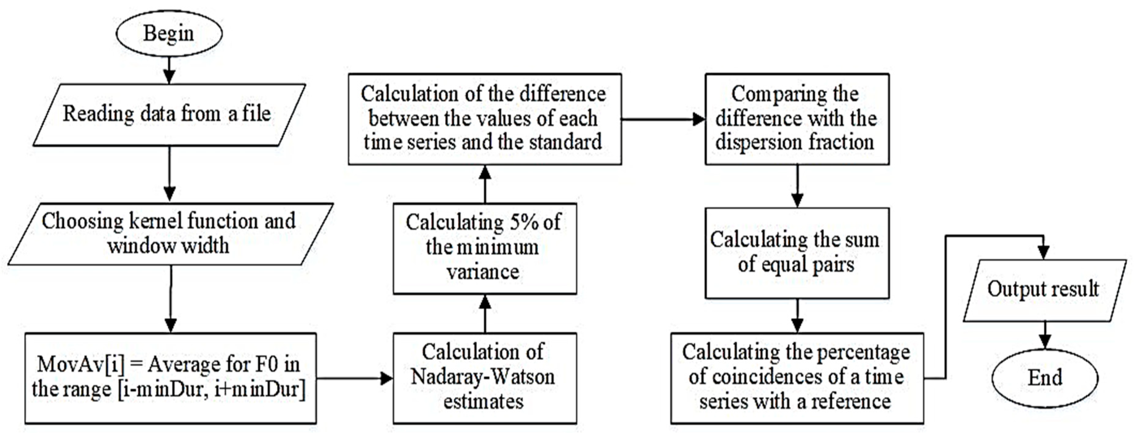
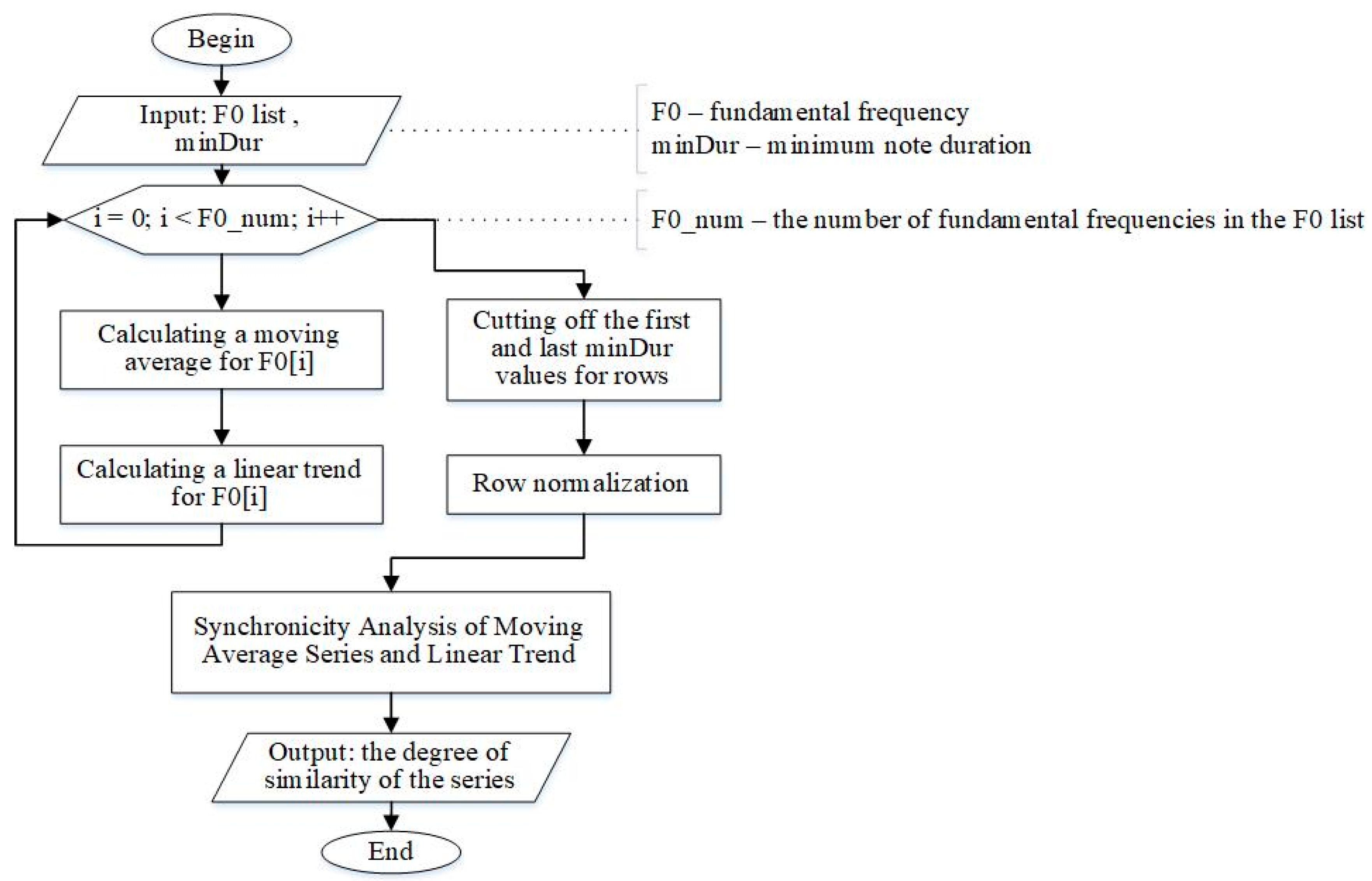
As a result, the software implementation of the algorithm for assessing the similarity of vocal performances was performed (
Figure 2).
The developed algorithm for assessing the similarity of vocal performances, based on the use of the synchronicity extraction metric, contains two stages. At the first stage, the reference and estimated frequency series are approximated; the second stage consists of comparing each value of the approximated estimated series with the corresponding value of the approximated reference series, determining the number of equal pairs and calculating the proportion of coincidences of the time series with the reference. Previously, this algorithm was used to analyze meteorological data [
49].
When investigating the error values choosing different kernels, the following recommendations were made: for triangular, trisquare and tricubic kernels, the window width should be 2. For the rest of the kernels, the window width is 1. The minimum errors were obtained with the Vallée-Poussin kernel and were less than 5%.
Table 1 shows the results of assessing the similarity of vocal performances of each location by each performer. As can be seen from the results obtained, locations 1, 2, 7 and 8 are most accurately executed—the degree of similarity is over 90%, and the results are almost the same for all types of kernels. The differences in the choice of kernels are especially noticeable for evaluating the performance of locations 4 and 6—the use of the Vallée-Poussin and Fisher kernels noticeably increases the degree of similarity for all performers. The best core results for each location sung by the performer are highlighted in bold text.
When listening to the performances, the fourth and sixth locations are indeed performed worse by almost all singers, but their degree of similarity is quite high—more than 50%. Considering that the accuracy of the assessment with the Vallée-Poussin kernel is higher than that of the others, the results obtained show that this method of assessing the degree of similarity using Vallée-Poussin or Fischer kernels can be further developed and used to determine the similarity of vocal performances.
One of the options for using this method of assessing similarity can be to check the quality of the task of performing a sequence of notes when teaching vocals. As indicated in [
50], hitting a note depends on the pitch of the voice, which is the sum of the physiological characteristics of a person [
51]. It is because of these features that a person may not fall into a certain octave of a note. In the initial stages of learning to sing, this should not be taken as a mistake, since the note is sung correctly. Therefore, at the initial levels of training, it is necessary to assess the dynamics of F
0.
5. Vibrato and Glissando Identification in Vocal Performance
5.1. Approach to Vocal Performance Analysis
The tests of the algorithm showed that when processing audio recordings, including various approaches to playing notes in the range from 70 to 800 Hz, the software complex allows you to recognize more than 95% of the notes sung by the speaker. It was determined that when singing arpeggio, crescendo and decrescendo, there is no effect on the quality of the algorithms in the software. The lack of influence on the quality of note identification lies in the fact that the algorithm considers only the frequency of the fundamental tone in the analysis and the specifics of the operation of one of the stages of the note identification algorithm, which is responsible for determining the belonging of a voiced section to a note, lies in the focus on pure performance.
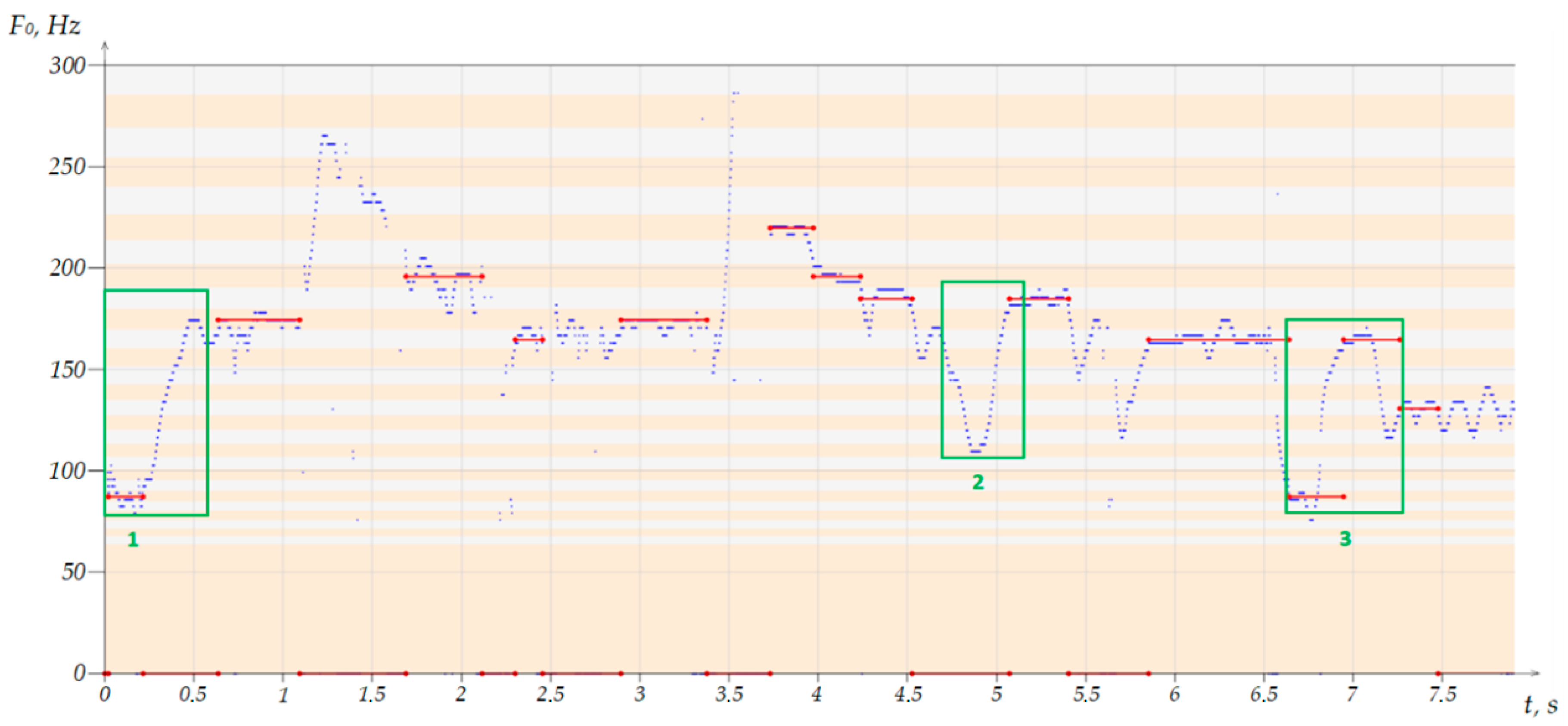
It is quite difficult to play a note so that all frequencies at the moment of singing are within the band allocated for it. For this reason, adjacent notes above and below the played one are considered. In
Figure 3,
Figure 4 and
Figure 5, the frequency spectrum is divided into sections corresponding to the boundaries of the notes. Each area is highlighted with a horizontal bar in the background of the frequency graph. The
X-axis is time, and the
Y-axis is the fundamental frequencies.
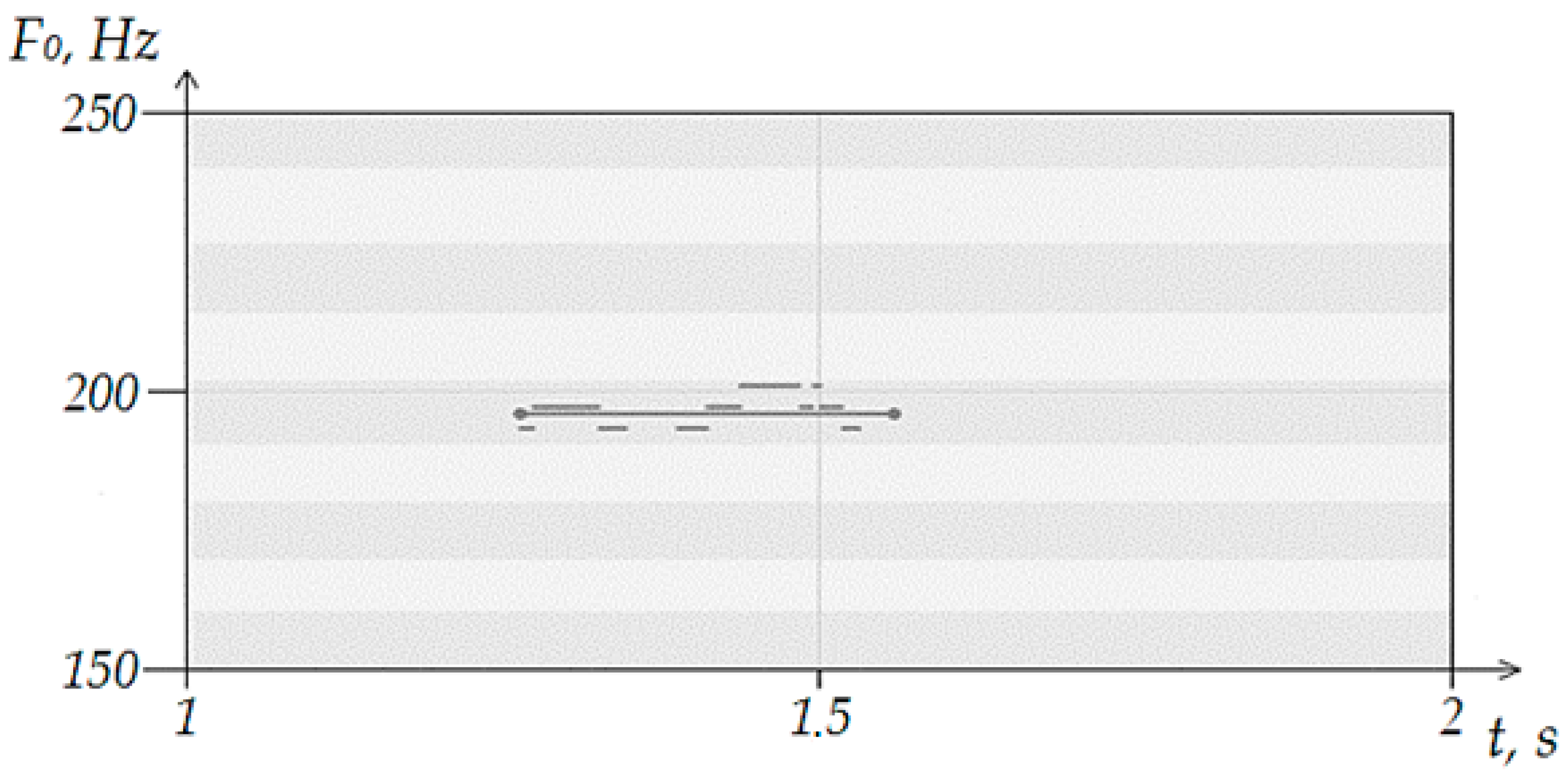
As you can see in
Figure 3, a segment sung within one note was recognized by the program. The number of moments found in adjacent notes is insignificant and did not affect the identification result. The overwhelming majority of recognized fundamental frequencies were in the range of the sung note. Considering the requirements for the accuracy of execution prescribed in the algorithm, the program was able to draw a conclusion about the sung note. If the number of fragments in each of the three sections turned out to be approximately the same, the algorithm perceives the entire voiced segment as noise.
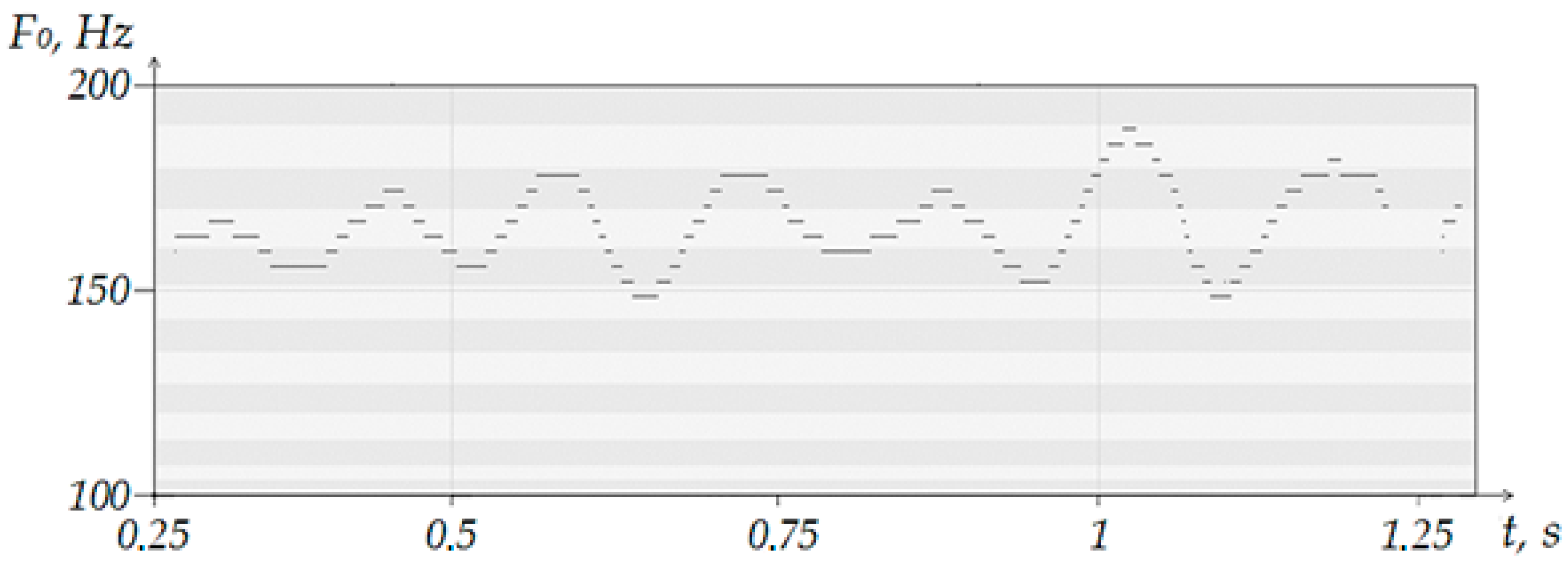
When singing vibrato, fluctuations occur in the frequency of the sound relative to a certain main note within a semitone. It should be noted that there are varieties of vibrato-like vibrations. This includes tremolation and voice swing. Due to the fact that the algorithm is set to detect clean notes, such segments are perceived as noise. As can be seen, the fluctuations during the performance of the main note (in this case, the note “minor octave E”) cover four notes at once. Considering the minimum duration of the sounding of a note leads to the fact that for each of the four notes, the singing within its boundaries took an insufficient amount of time. In this case, the return to this note occurs after the transition to other notes, which reduces the proportion of frequencies related to the main note.
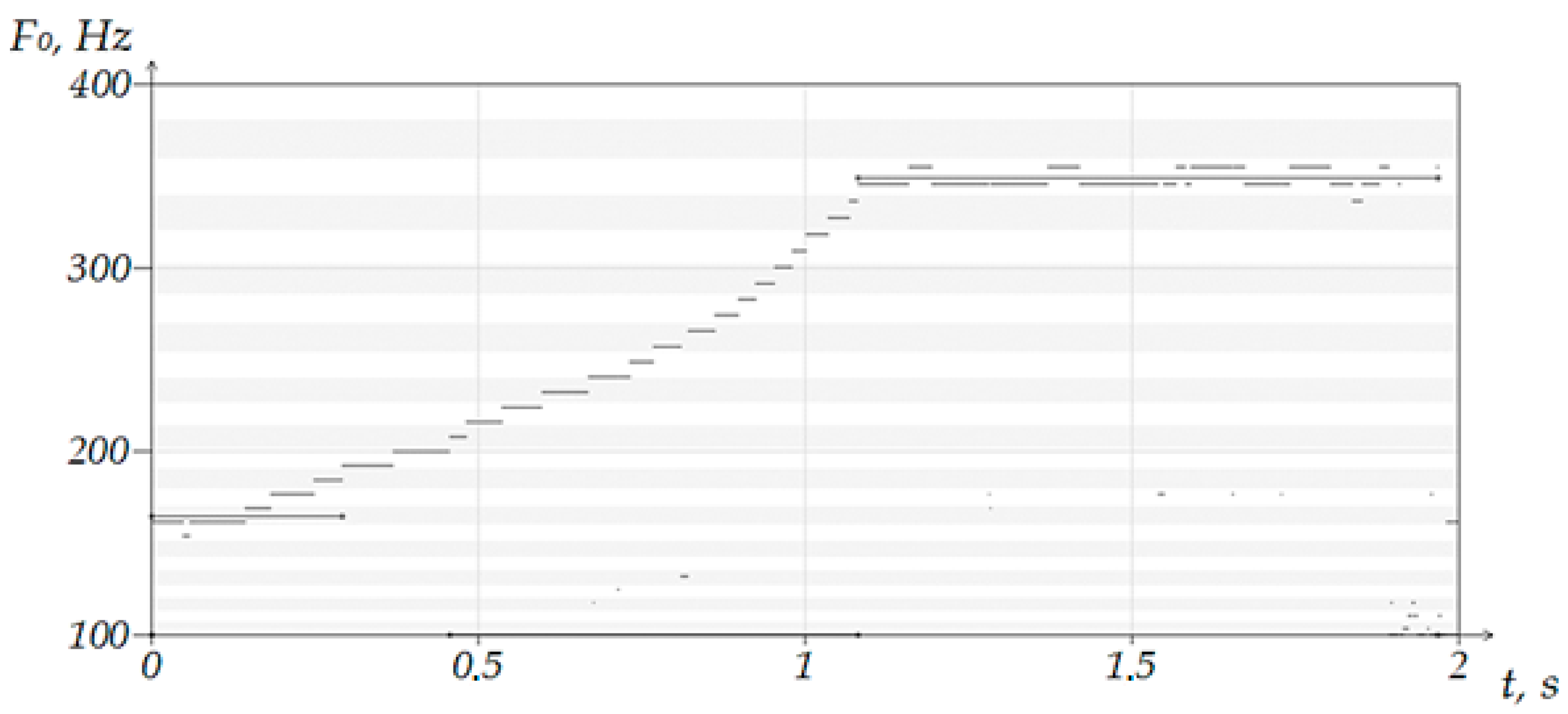
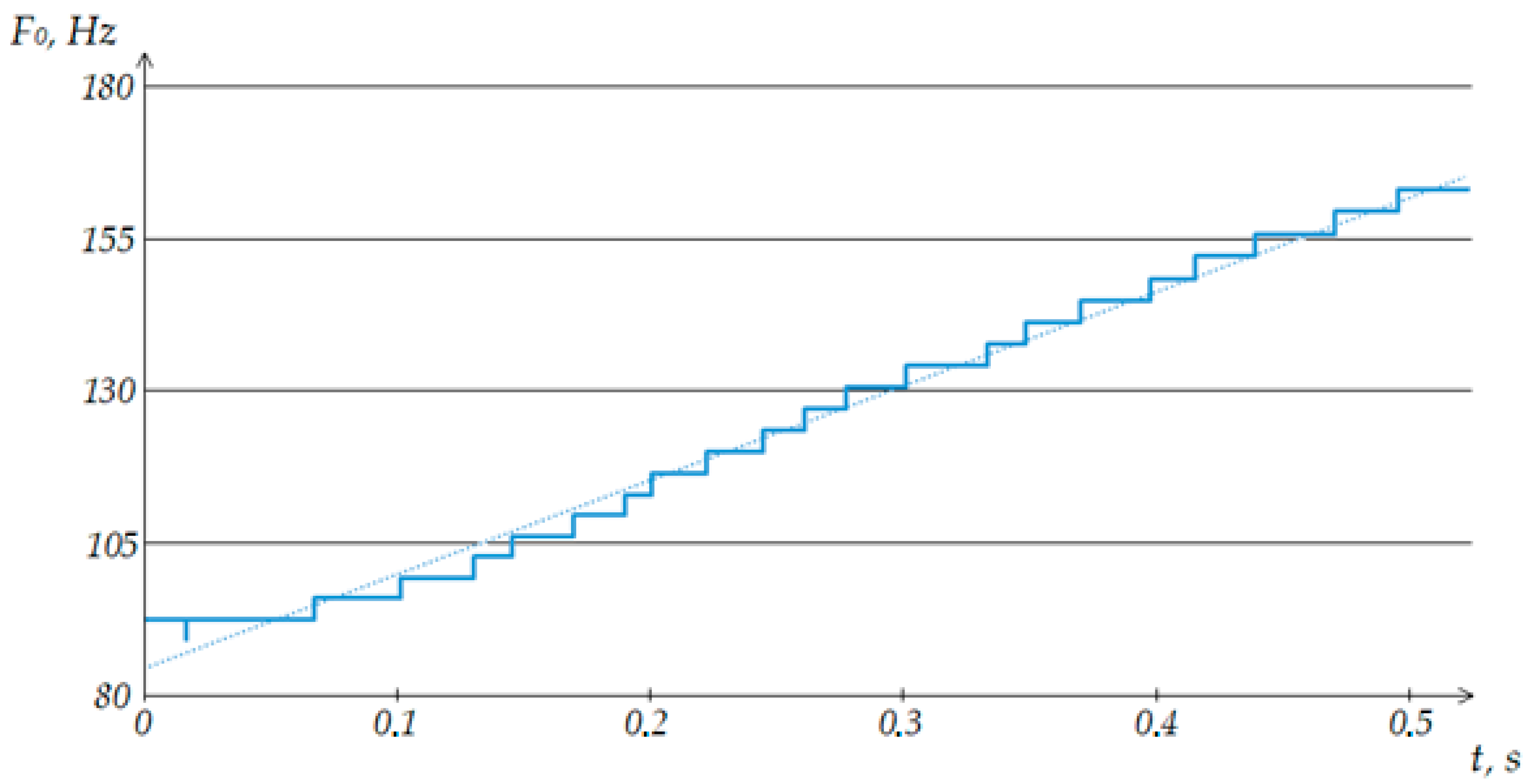
Another example of adding a coloristic effect to singing is such a technique as glissando. As is known from music theory, when singing a glissando, there is a smooth glide from one note to another. With this singing, the transition occurs too quickly in order to be able to identify each individual note at the moment of sliding, since there is less than 0.1 s for each segment of the covered notes. Glissando can be either ascending (as shown in
Figure 5) or descending. As can be seen in the figure, the algorithm is able to determine the start and end notes between which it is sliding. However, the coverage of 12 notes in between is perceived as noise.
Thus, it becomes necessary to identify areas perceived by the program as noise. We will assume that a directed transition from one note to another is a glissando, and oscillations relative to one note within a single segment are tremolation. Determining the type of tremolation will not be considered at this stage.
Since the array of found fundamental frequencies, within which it was not possible to identify a pure note, can be perceived as a time series, it was decided to conduct a preliminary analysis of the data. Among the preliminary analysis procedures, there are anomaly search, time series smoothing, trend checking and calculation of process dynamics indicators.
From the point of view of the considered subject area, anomalous observations can be perceived as bursts of frequencies determined outside the sound of the main melody. This includes any noise that the algorithms filter out during the note segmentation stage. Accordingly, this procedure can be considered completed.
As part of smoothing the time series, the true levels of the series are computed by the calculated values that have smoother dynamics than the initial data. It was decided to focus on the methods of mechanical smoothing, since in the problem under study it is necessary to evaluate each individual leveling of the series considering the actual values of the levels adjacent to it. The weighted moving average method is inapplicable for the problem under study, since it cannot contain a quadratic or cubic trend. Further, there is no need to use the exponential smoothing method, since it is used in the problems of predicting the development of the process after the study area. In this regard, the simple moving average method will be used according to the formula
where
is the number of observations included in the smoothing interval; and
is the number of observations on opposite sides from the smoothed.
As the number of observations included in the smoothing interval, it was decided to use the value of the minimum duration of the sounding of a note, used in the algorithm for the segmentation and identification of notes. The choice is due to the fact that when singing vibrato and glissando, the duration of singing within such sections is significantly higher than this parameter, but the identification of individual clean notes was not carried out by the basic algorithm. The disadvantage of the method is that the first and last observations will remain unsmoothed, which can be neglected due to the total duration of the estimated area.
Testing for the presence of a trend is essentially a test of the hypothesis that the mean value of the time series remains unchanged. For testing, a series can be divided into n parts, each of which is considered as a separate set. The resulting averages for each population will be compared. If the average values increase or decrease, we will assume that the segment under study may contain a glissando (ascending or descending, respectively).
All preliminary calculations were carried out in Microsoft Excel. The built-in functionality contains the “Data Analysis” function, in which a moving average can be plotted for the selected series.
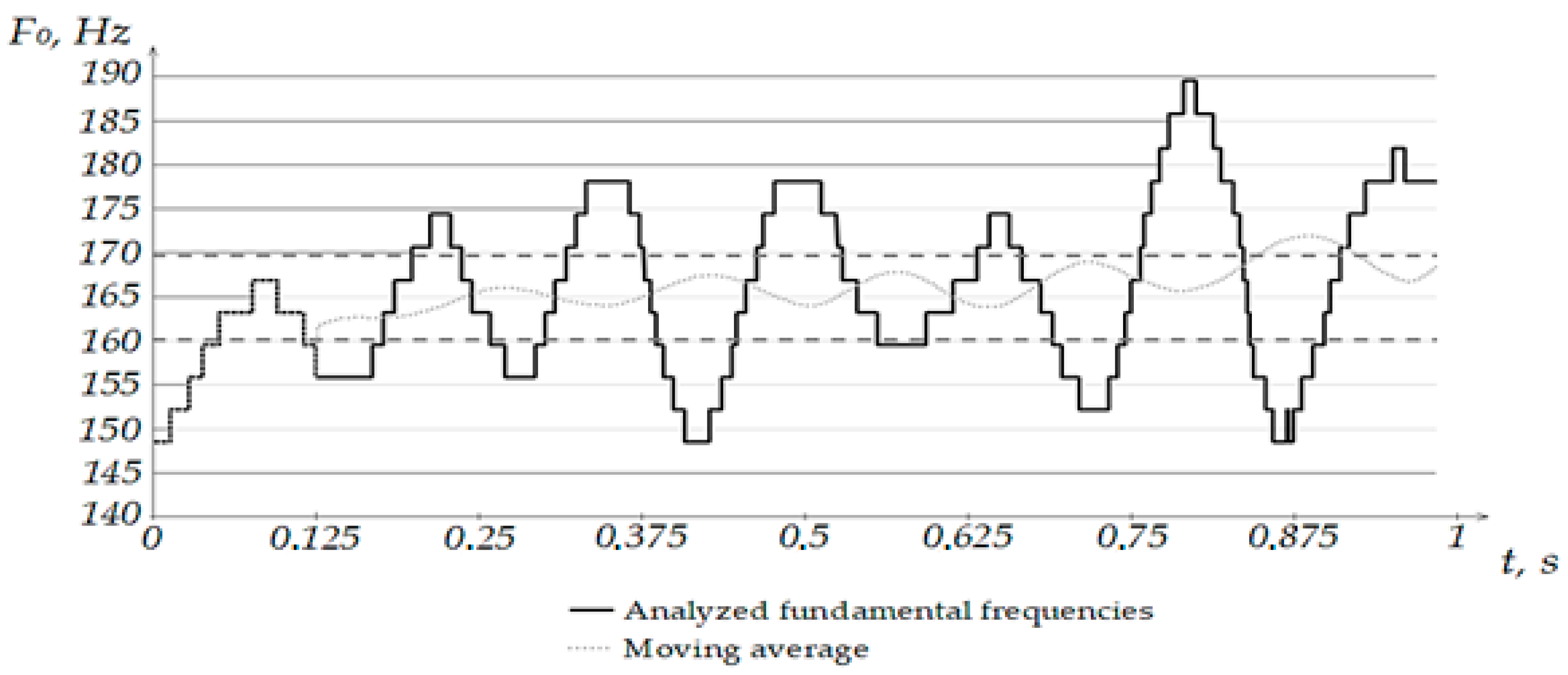
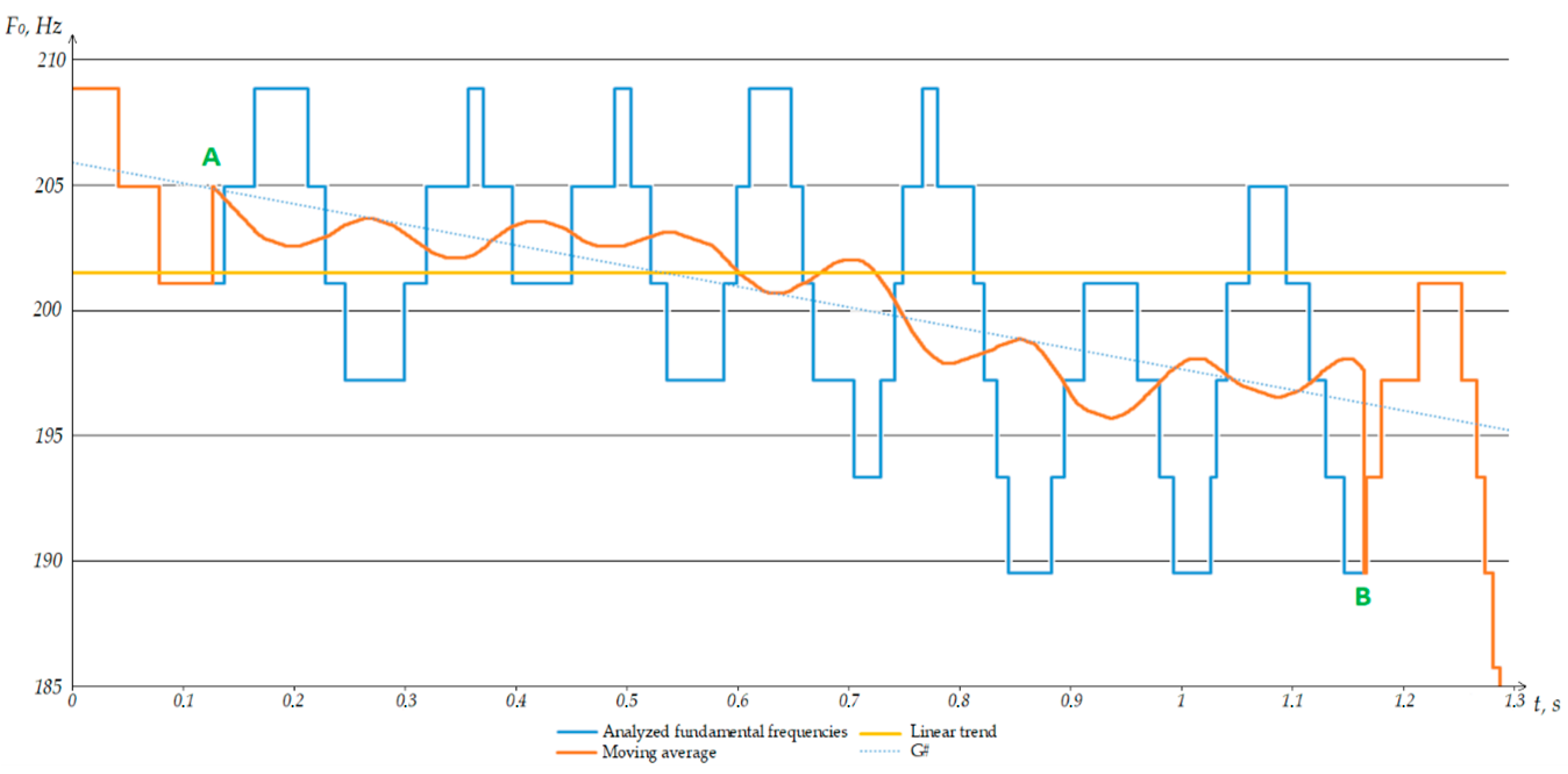
Figure 6 shows the result of applying this method. In the built-in method, only the previous values are analyzed, without considering the following after the estimated one, which makes it possible to obtain an envelope curve that is uninformative within the framework of the study. In order to solve this problem, the classical formula of sliding smoothing was used, considering the measurements before and after the smoothing one, with 0.5 *
values preceding the smoothing one, and the same number of subsequent values was included in the smoothing interval (
Figure 6). As a result, at the interval from 0 to 0.5 *
p, the values of the series will coincide, but starting from the next value, we will be able to see the averaging. The solid line indicates the values of the analyzed fundamental frequencies, and the dashed oscillating line indicates the smoothed values.
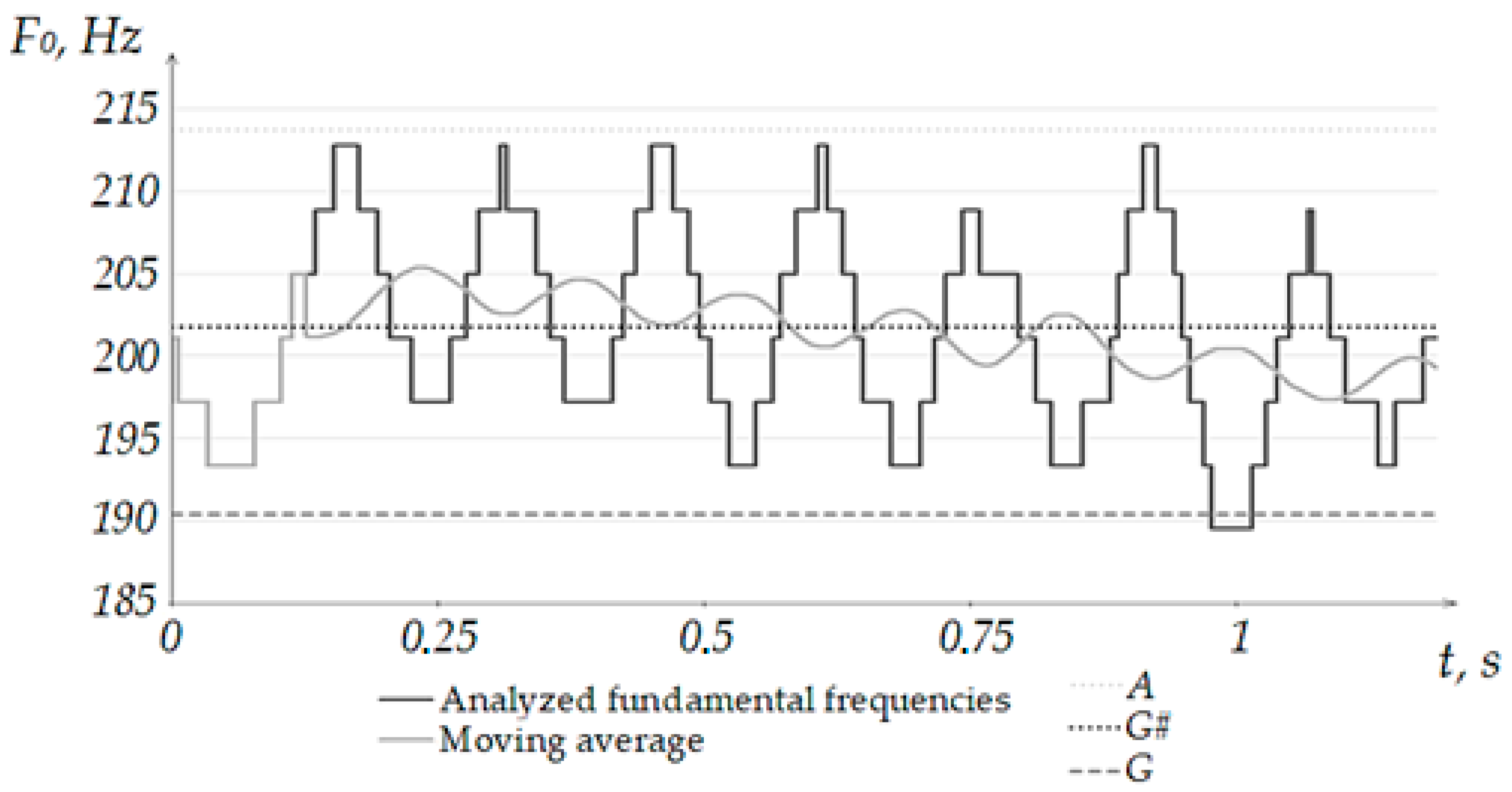
In the figure presented, for the note “minor octave E”, parallel dashed lines indicate the lower (160.121 Hz) and upper (169.643 Hz) sounding limits, determined using the logarithmic average. Note that in the studied segment, there are seven oscillations in the frequency of the fundamental tone, judging by the graph. On further investigation of the type of vibration in singing, this aspect can be used as a criterion for distinguishing vibrato from tremolation.
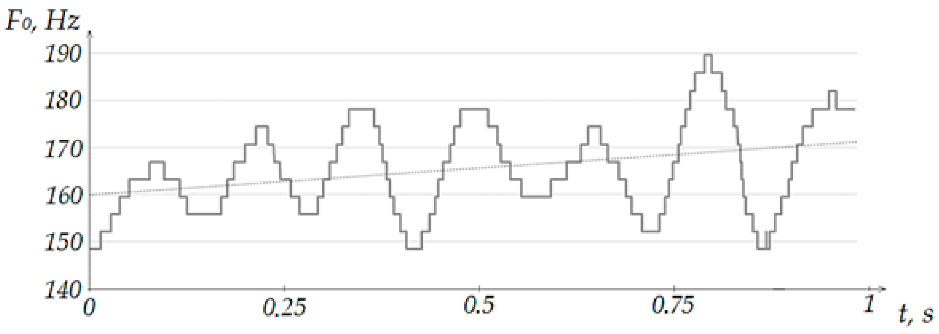
As mentioned earlier, the presence of a trend is determined by comparing the obtained mean values for each of the sets of the studied series. Further, by means of Excel, on the graph of the fundamental frequencies for the series, one can set the construction of a linear trend (
Figure 7). At the stage of analyzing the applicability of the method to the problem under study, we will use the built-in function in Excel, and at the stage of implementation in the software package, we will compare the average values for segments of the studied range.
As can be seen from the figure above, the linear trend allows one to determine that in most of the surveyed area, the average frequency values refer to one note. However, it is impossible to assess the presence of fluctuations in the fundamental frequencies from a linear trend. In this regard, it is not possible to use only a linear trend for assessing areas with tremolation. The trend allows you to estimate the number of notes covered in the study area, but not the type of performance. In turn, the moving average simultaneously interprets both the presence of vibrations and the covered notes, which makes this estimation method more preferable for vibrato-like areas.
To determine the glissando in the studied area, one must complete another task. The basic algorithm for the segmentation and identification of notes determines two notes in such situations: the one with which the slip began, and the one at which the slip ended. Accordingly, the first task to be solved to determine the presence of glissando is to compare notes at the boundaries of the area under study. If the notes turn out to be identical, then the area between them cannot correspond to the glissando and should be considered for attribution to vibrato. In other cases, we will observe a trend line passing through several notes. The greater the difference between the notes and the faster the transition between them, the greater the angle of the resulting trend line relative to the time axis.
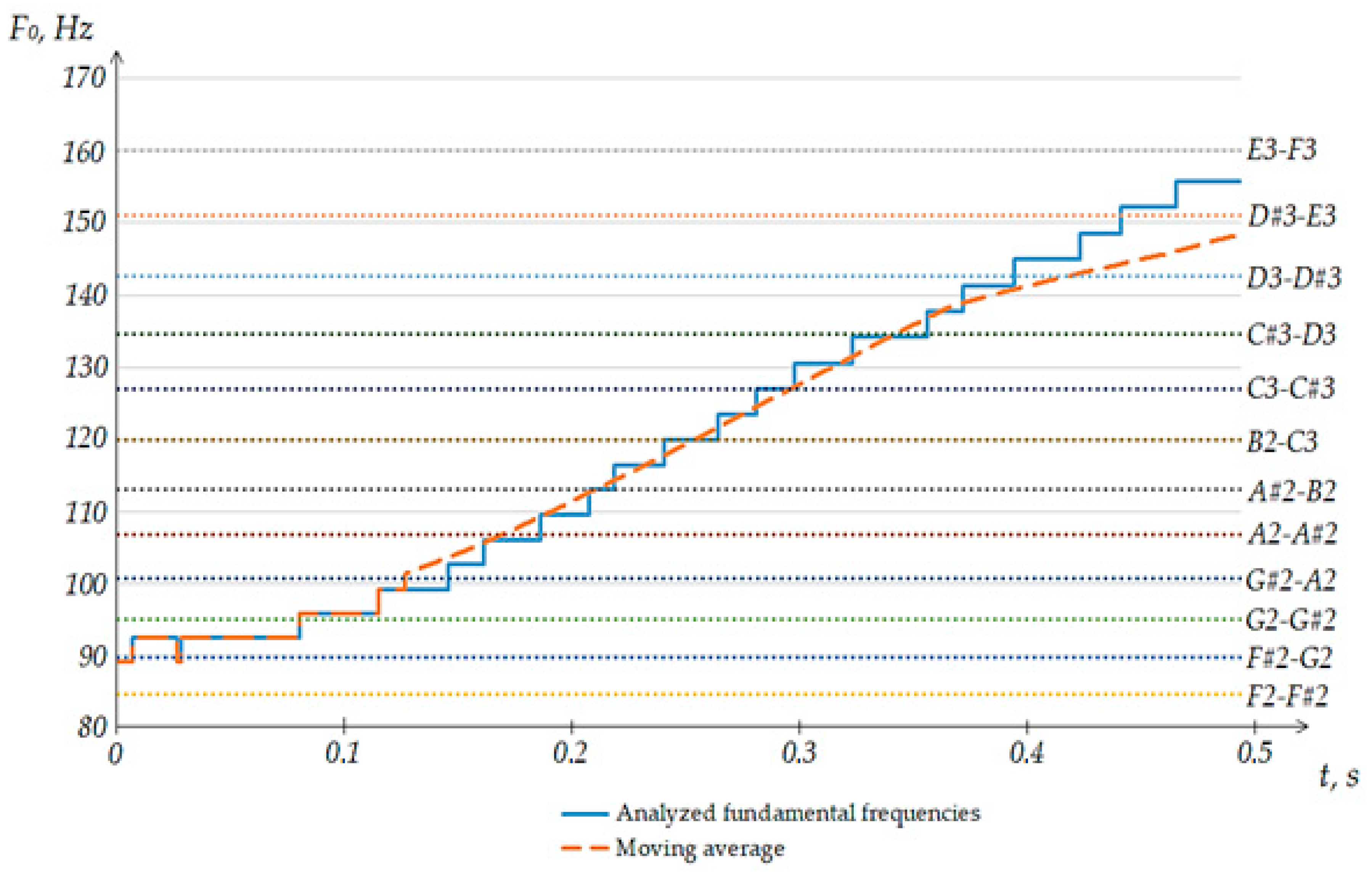
As for the tremolation section, consider the moving average for the range under study. As can be seen in
Figure 8, there are no obvious fluctuations in the frequency of the main tone in the transition from the note “minor octave G” to the note “1st octave E”. The solid line on the graph indicates the fundamental frequencies, and the dashed line indicates the moving average for the range under study. Parallel dotted lines correspond to note boundaries. The resulting moving average line goes through nine notes. Thus, the data obtained indicate an ascending glissando. Below (
Figure 9) is a graph for a linear trend obtained on the studied range. In fact, the linear trend for the range under study is close to the result obtained when plotting the moving average.
As can be seen from the results obtained, when using a moving average for areas with tremolation, an oscillation effect is observed that is absent in the linear trend for this area. On the other hand, for the glissando, the moving average and the linear trend behave in a similar way. This allows us to apply both methods in an integrated manner to determine the current situation.
The proposed idea is to obtain both estimates for the segment under study. The resulting datasets will be compared for the degree of similarity between their estimates for a certain parameter . The size of the value of this parameter requires a separate experiment. Within the framework of this experiment, mixed situations should be considered, in which the time series behave ambiguously, in order to reduce the number of errors of the first and second kinds when determining the type of the studied fundamental frequency ranges.
If there was a glissando in the singing, the results of the moving average and linear trend for the given time series will be close. For this situation, it will be necessary to check for the number of notes through which the transition was made, and the direction of the transition (ascending or descending glissando). As a result, it will be possible to filter out areas with noise between adjacent segments corresponding to one note and areas with a burst of noise outside the range between notes.
For situations in which the difference in the estimates of the time series will exceed the value of the criterion, we will assume that there was singing with vibrato in the voice. As noted earlier, the moving average has a wave-like structure in the case of fluctuations in the studied area. Counting the number of oscillations per unit of time can be used in the classification problem of the tremolation type. This parameter will be useful when teaching vocal performance in case of too frequent or rare fluctuations in the performance of a note. In addition, in the case of detecting vibrato in singing, it will also be necessary to control the number of notes through which the trend passed. As can be seen in
Figure 10, the oscillations for the sung note slide downward. In fact, in this example, glissando and vibrato are mixed. However, this section cannot be attributed to any of the types for two reasons: the presence of vibrations in the voice is not typical for glissando, and for vibrato, there should be no slips to another note.
5.2. Description of the Collected Audio Database
As a material for calculating the values of the moving average and linear trend, audio recordings with vocal performances by students of a music studio were considered. Each student was given the task to listen to the reference recording and make five recordings with the singing of the assigned task. In total, 17 master records and 740 student records were collected, containing a total of 13,078 sung notes. The database contains recordings with different ranges of notes, sung by both male and female voices of different ages. The duration of the audio recordings varies from 2 to 20 s, depending on the exercise performed by the speakers.
Each of the collected audio recordings has the following parameters:
Each of the audio recordings was segmented into separate notes and sections, within which the notes were not identified. Sections with vibrato-like or glissando singing were separately identified. Each recording was rated by vocal teachers from the music school. The consistency in expert estimates for the audio recordings was checked using the Kendall coefficient. Further evaluation was carried out in accordance with the exhibited expert assessments.
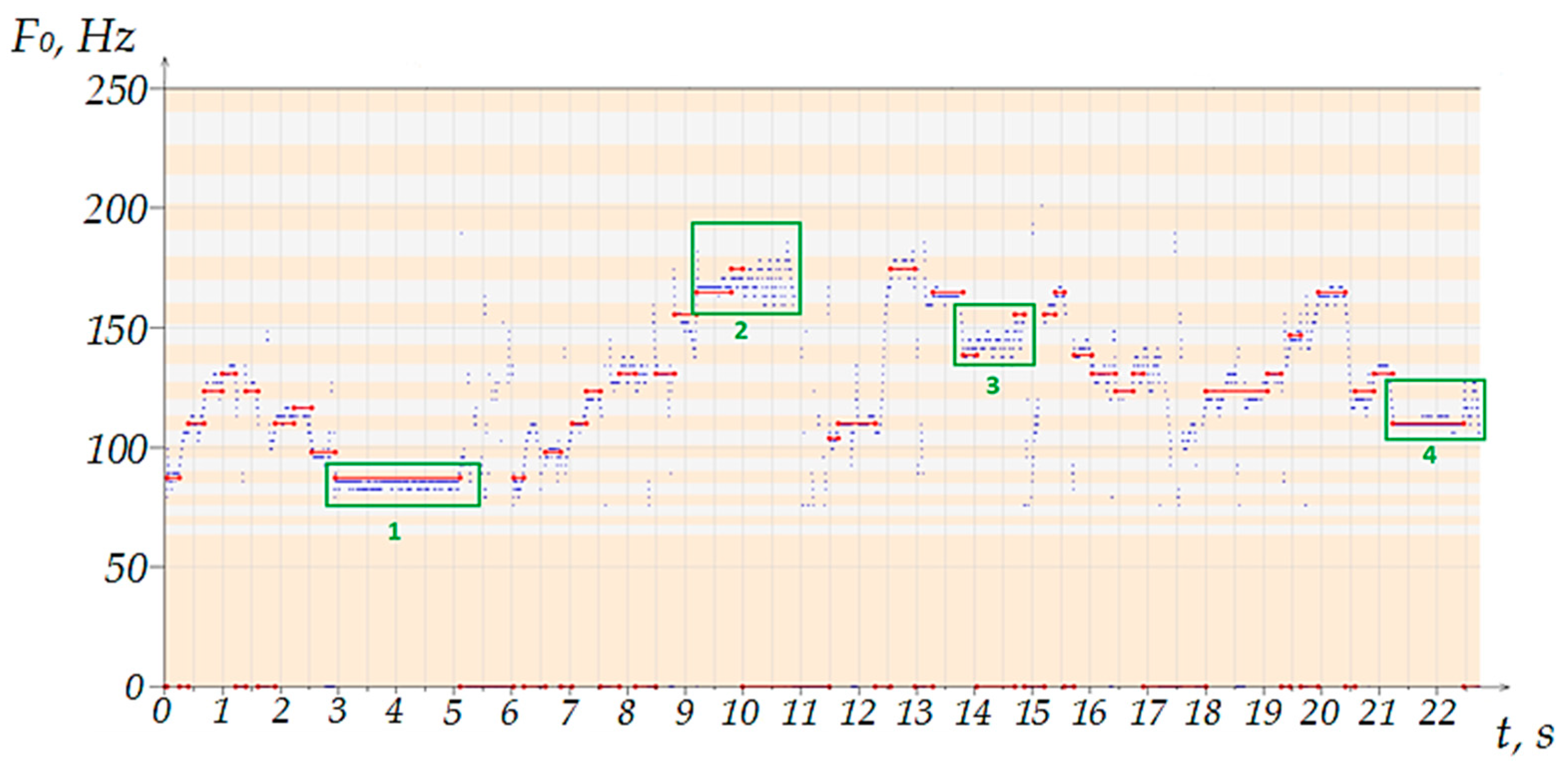
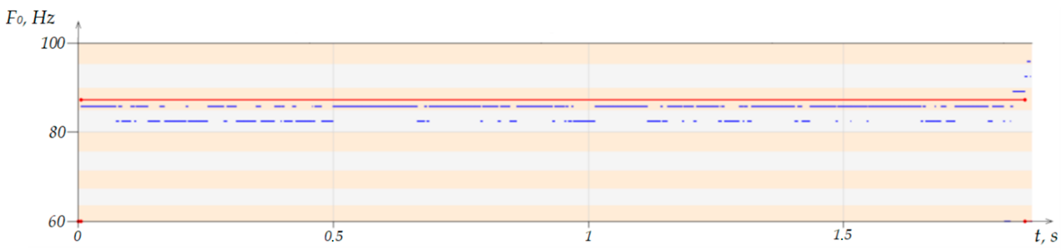
Figure 11 shows an example with four highlighted areas corresponding to singing with vibrato in the voice. As can be seen, in
Section 1, fluctuations occur within one note (
Figure 12), which made it possible to identify the note. A similar situation is observed in the fourth section.
Despite the fact that the presence of vibrations in the voice did not affect the accuracy of recognizing notes in the situations considered, it was decided to re-examine such areas in order to find possible distinguishing features that would allow us to classify similar segments. This will help to not only more accurately recognize notes with fluctuations, but also consider the intentional transitions to adjacent notes when assessing the quality of singing. In addition, similar segments will not be overlooked in the analysis phase of the vibrato-like performance type.
Figure 13 shows an example with segmented sections containing an upward glissando. As can be seen for segments 1 and 3, the note recognition algorithm was able to identify the initial and final values of the notes between which the slip occurs, and the frequencies between them are perceived as noise. For segment №2, the starting moment of the ascending glissando is also the final one for the descending one from the previous note.
A total of 740 audio recordings were segmented into 149 vibrato-like singing sections and 68 glissando sections, of which 54 were ascending and 14 were descending. The duration of the audio recordings varies from 0.5 to 3 s. For each audio recording, the values of the fundamental frequencies were obtained, which were preliminary estimated manually in MS Excel using the functions described above.
5.3. Analysis of Audio with Vibrato and Glissando Singing
Within the framework of the software package [
52], a module was developed that is responsible for the analysis of the selected fundamental frequency range. The algorithm of the module is shown in
Figure 14. The module receives an array with the fundamental frequencies of a segment that is not recognized by the note recognition algorithm and is considered for the presence of tremolation or glissando transition between notes. In addition, it is necessary to inform the module about the minimum duration of the sounding of notes, corresponding to the considered audio recording.
For the investigated array of frequencies, using Formula (17), an array is formed with the values of the moving average at each moment of time in the studied range. When calculating the values of the linear trend at each time point, the least squares method was used.
Since the initial and final observations of the moving average remained equal to the initial values of the fundamental frequencies, the series of the moving average and linear trend were cut off at the first and last values. The remaining values were normalized and processed using the synchronicity extraction metric. The evaluation of the similarity of time series by the metric is launched by calling the subroutine. For each selected audio recording, the fundamental frequencies were calculated and analyzed using the developed module.
5.4. Audio Processing Results
A fragment of the experimental results is presented in
Table 2.
Analysis of 217 audio recordings showed that glissando has a 5 to 15% synchronicity rate between a linear trend and a moving average, while vibrato singing has a range of 65 to 85%. At the same time, the cleaner the vibrato singing, the higher the percentage of discrepancy between the series. For glissando, on the contrary, the lower the percentage, the less side frequencies there were when switching to singing. In addition, 67 recordings with a combination of vibrato and glissando in singing were processed. The mixed types of singing described before
Figure 10 are perceived by the method as 45–50% different.
Figure 15 shows an example in which a mixture of vibrato in singing with a transition to a lower note leads to the impossibility of identifying separately each of the applied singing methods. The presence of a trend towards a decrease or increase in the overall sound of a segment in the frequency domain leads to a smoother change in the moving average for the area under study.
The results obtained make it possible to automate the assessment of areas that were not recognized by the basic algorithm for recognizing notes in vocal performance. By dividing the range of accepted results from the method of separating the synchronicity of time series into sections, it is possible to unambiguously classify areas with a sharp change in the fundamental frequency. If the difference is no more than 15%, one can assume that there is a glissando in the singing of the treated area. With estimates in the range from 65% to 85%, we will assume that the studied segment was sung with vibrato-like vibrations. Intermediate values (from 16 to 64%) will be perceived as noise.
6. Conclusions
In the course of this study, a metric for assessing the degree of similarity of time series was developed and applied. This metric makes it possible to consider the assumptions about the model of the series and to compare the values of the corresponding characteristics. The sphere of speech technologies was chosen as an area of application of this approach for assessing the similarity of time series. Tests were carried out with the values of the fundamental frequencies of vocal performances in several directions.
One of the directions for assessing the similarity of vocal performances was the comparison of the functions of the dependence of fundamental frequencies on time for several speakers. As a test, one speaker was given the task to sing a sequence of notes, and the rest of the speakers were given the task to reproduce the melody they heard. It was determined that the use of the synchronicity allocation metric allows for an exercise in which students need to repeat the melody after the teacher. This teaching model is the closest to that implemented in the framework of teaching singing in music schools.
Another application of the synchronicity extraction metric is the implementation of an algorithm for identifying segments with a sharp change in fundamental frequencies. The tests of the software complex showed that the note recognition algorithm is able to identify up to 95% of the notes sung by the speaker. The exceptions are notes played with glissando and vibrato. The basic algorithm of the program considered only clean notes, which did not allow identifying vocal performances with a sharp change in frequencies. For the analysis of unrecognized areas, the synchronicity detection metric was applied to the time series estimates. It was determined that glissando is characterized by a high degree of similarity for the linear trend and the moving average for the study area, while the opposite is true for vibrato. For vocal performances with tremolation, differences from 65 to 85% are characteristic.
The results obtained show that the use of the synchronicity extraction metric in the analysis of speech signals allows one to determine the similarity of both several speech signals and estimates of the behavior of the fundamental frequency for one recording. This will allow the described metric to be considered in other studies. One of the applications can be the use of the metric in the task of identifying a speaker. In this direction, it is possible to evaluate the similarities of the reference recording with the speaker’s voice to the recordings of a legal user and intruders, as well as the signal parameters determined by the articulators of different speakers.
This work is devoted to the study of the possibility of identifying singing with a sharp change in fundamental frequencies. Within the framework of the described study, the features of the software package are redundant. A detailed description of the applied algorithm for identifying notes in vocal performance and the obtained test results will be published as part of a further study.


