Generation of Julia and Mandelbrot Sets via Fixed Points

Abstract

The aim of this paper is to present an application of a fixed point iterative process in generation of fractals namely Julia and Mandelbrot sets for the complex polynomials of the form $T\left(x\right)=x^n+mx+r$ where $m,r\in \mathbb{C}$ and $n\ge 2$. Fractals represent the phenomena of expanding or unfolding symmetries which exhibit similar patterns displayed at every scale. We prove some escape time results for the generation of Julia and Mandelbrot sets using a Picard Ishikawa type iterative process. A visualization of the Julia and Mandelbrot sets for certain complex polynomials is presented and their graphical behaviour is examined. We also discuss the effects of parameters on the color variation and shape of fractals.

1. Introduction

Fixed point theory provides a suitable framework to investigate various nonlinear phenomena arising in the applied sciences including complex graphics, geometry, biology and physics [1,2,3,4]. Complex graphical shapes such as fractals, were discovered as fixed points of certain set maps [1]. Informally, fractals can be treated as self similar mathematical structures which have similarity and symmetry such that considerably small parts of the shape are geometrically akin to the whole shape. Fractals are also known as expanding symmetries or unfolding symmetries. Although, fractals do not have a formal definition, however they are identified through their irregular structure that cannot be found in Euclidean geometry. Julia [5] who is considered as one of the pioneers of fractal geometry, studied iterated complex polynomials and introduced Julia set as a classical example of fractals. Let $\mathbb{C}$ be the complex space, $T:\mathbb{C}\to \mathbb{C}$ be a complex polynomial of degree $n\ge 2$ with complex coefficients and $T^i\left(x\right)$ be the $i^{th}$ iterate of x. The behaviour of the iterates $T^i\left(x\right)$ for large i determine the Julia set (see [1,6,7,8]).

Definition 1

([1]). The set of points in $\mathbb{C}$ whose orbits do not converge to a point at infinity is known as filled Julia set, $K_T$, that is,

$$K_T=\left\{x\in \mathbb{C}:\left\{\right|T^i\left(x\right){\left|\right\}}_{i=0}^{\infty }\mathit{is}\mathit{bounded}\right\}.$$

Julia set of T denoted by $J_T$ is the boundary of filled Julia set, that is, $J_T=\partial K_T$.

Therefore, we may say that $x\in J_T$ if for every neighborhood of x there exist points w and v such that $T^i\left(w\right)\to \infty$ and $T^i\left(v\right)\nrightarrow \infty$. The complement of a Julia set is a Fatou set.

Let $p\in \mathbb{C}$ be a fixed point of T and $|{\left(T^i\right)}^{\prime }p|=\rho$, where prime denotes the complex differentiation. A point p is called a periodic point if $p=T^{i}p$ for some integer $i\ge 0$. Let $\left\{p,Tp,\dots ,T^{i}p,\dots \right\}$ be an orbit of p. The point p is called an attracting point if $0\le \rho <1$ and a repelling point if $\rho >1$ [6,7]. The following result gives a significant connection between repelling points of a polynomial and the Julia set.

Theorem 1

([6]). If T is a complex polynomial, then $J_T$ is the closure of the repelling periodic points of T.

Let p be an attracting fixed point of T. Then, the set $A\left(p\right)$ is called the basin of attraction of p if

$$A\left(p\right)=\left\{x\in \mathbb{C}:T^{i}x\to p\mathrm{as}i\to \infty \right\}.$$

The basin of attraction of infinity, $A(\infty )$, is defined in the same way. The following lemma is pivotal in determining Julia sets.

Lemma 1.

[7] Let p be an attracting fixed point of T. Then, $J_T=\partial A\left(p\right)$.

Thus, the Julia set is the boundary of the basin of attraction of each attracting fixed point of T, including ∞. The existence of the fixed point p for any complex polynomial is guaranteed by Brouwer fixed point theorem [9]. However, the existence of an attracting fixed point depends on the choice of the parameters. Consider the polynomial $Q_r\left(x\right)=x^2+r.$ Then it has two fixed points excluding infinity. In this case, a fixed point p is attracting if $\left|2p\right|<1$ i.e., $|1-\sqrt{\frac{1}{4}-r}|<1$. Fix $v_r=\sqrt{\frac{1}{4}-r}$, then the set of parameters r such that $Q_r$ has an attracting fixed point is given by $S=\left\{r\in \mathbb{C}:|1-v_r|<1\right\}$. Julia sets, $J_{Q_r}$, on the real axis i.e., $r=0$ are reflection symmetric while those with complex parameter values, $r\in \mathbb{C}$ demonstrate rotational symmetry.

Mandelbrot [10] extended the idea of Julia sets and presented the notion of fractals. He investigated the graphical behaviour of connected Julia sets and plotted them for complex function, $Q_r\left(x\right)=x^2+r$, where $x\in \mathbb{C}$ is a complex variable and $r\in \mathbb{C}$ is an input parameter. He noted that various geometrical properties involving dimension, symmetry and similarity play consequential role in the study of fractal geometry.

Definition 2

([6]). Let T be any complex polynomial of degree $n\ge 2$. A Mandelbrot set M is the set consisting of all parameters r for which the Julia set, $J_{Q_r}$, is connected, that is,

$$M=\left\{r\in \mathbb{C}:J_{Q_r}\mathit{is}\mathit{connected}\right\},$$

or an equivalent definition is

$$M=\left\{r\in \mathbb{C}:\left\{\right|Q_r^n\left(0\right)\left|\right\}\nrightarrow \infty \mathit{as}n\to \infty \right\}.$$

Mandelbrot [10,11] noted that records of heart beat, irregular coastal structures, variations of traffic flow and many naturally existing textures are examples of fractals.

In order to generate and analyze fractals, various techniques are used such as iterated function systems, random fractals, escape time criterion etc. The escape time algorithm is the stopping criterion that is based on the number of iterations necessary to determine if the orbit sequence tends to infinity or not. This algorithm provides a suitable mechanism used to demonstrate some attributes of dynamic system under iterative process. Generally, the escape criterion for Julia and Mandelbrot sets is given by:

Theorem 2

([6]). For $Q_r\left(x\right)=x^2+r$, $x,r\in \mathbb{C}$, if there exists $i\ge 0$ such that

$$|Q_r^i\left(x\right)|>max\left\{\left|r\right|,2\right\},$$

then $Q_r^i\left(x\right)\to \infty$ as $i\to \infty$.

The term $max\left\{\left|r\right|,2\right\}$ is also known as escape radius threshold. The escape radius varies in each iteration. The escape radius has a key role in visualizing the fractals.

Historically, Julia and Mandelbrot sets are investigated for the polynomials $Q_r$ but the study has been extended to quadratic, cubic, and $n^{th}$ degree complex polynomials. Lakhtakia et al. [12] explored the Julia sets for general complex function of the form $T\left(x\right)=x^n+r$ where $n\in \mathbb{N}$. The superior Julia and superior Mandelbrot sets for such complex polynomials in the context of noises arising in the objects were analyzed by Negi et al. [13,14]. Rochon [15] considered a more generalized form of Mandelbrot sets in bi-complex planes, see also [16,17].

Many authors have utilized various iterative processes to generate fractals. Julia and Mandelbrot sets have usually been studied for quadratic, cubic and higher degree polynomials in Picard orbit [8]. Let $T:\mathbb{C}\to \mathbb{C}$ and $x_0\in \mathbb{C}$. The Picard orbit [6] is a sequence $\left\{x_i\right\}$ which is given by

$$x_{i+1}=T\left(x_i\right),$$

where $i\ge 0$.

Since the convergence of Picard process is slow, various faster converging iterative processes have been introduced to generate Julia and Mandelbrot sets. Rani and Kumar [18,19] used one-step Mann iterative process to generate superior Julia and Mandelbrot sets for $n^{th}$ degree complex polynomials of the form $T\left(x\right)=x^n+r$. The Mann orbit, for any $x_0\in \mathbb{C}$, is a sequence $\left\{x_i\right\}$ which is given by

$$x_{i+1}=(1-\alpha )\left(x_i\right)+\alpha T\left(x_i\right),$$

where $i=0,1,\dots$ and $\alpha \in (0,1]$.

In 2010, a two-step Ishikawa iteration was used by Rana and Kumar [20] and Chauhan et al. [21] to study relative superior Julia and relative superior Mandelbrot sets, respectively. The dynamics of the nth order complex polynomial for non integer values were investigated in [22]. The authors also obtained new Julia and Mandelbrot sets via Ishikawa orbit. The Ishikawa orbit, for any $x_0\in \mathbb{C}$, is a sequence $\left\{x_i\right\}$ which is given by

$$\left\{\begin{array}{cc}{x}_{i+1}\hfill & =(1-\alpha )x_i+\alpha T{y}_i,\hfill \\ y_i\hfill & =(1-\beta )x_i+\beta T{x}_i,\hfill \end{array}\right.$$

where $i=0,1,\dots$ and $\alpha ,\beta \in (0,1]$.

Ashish and Rani [23] investigated the three-step Noor iteration process for Julia and Mandelbrot sets. The Noor orbit, for any $x_0\in \mathbb{C}$, is a sequence $\left\{x_i\right\}$ which is given by

$$\left\{\begin{array}{c}{x}_{i+1}=(1-\alpha )T{x}_i+\alpha T{y}_i,\hfill \\ y_i=(1-\beta )T{x}_i+\alpha T{u}_i,\hfill \\ u_i=(1-\gamma )T{x}_i+\gamma T{x}_i,\hfill \end{array}\right.$$

where $i=0,1,\dots$ and $\alpha ,\beta ,\gamma \in (0,1]$.

The modified Ishikawa process, S-iteration, was employed by Kang et al. [24,25] to study relative superior Mandelbrot sets, tricorn and multicorns. The S-orbit, for any $x_0\in \mathbb{C}$, is a sequence $\left\{x_i\right\}$ given by

$$\left\{\begin{array}{c}{x}_{i+1}=(1-\alpha )x_i+\alpha T{y}_i,\hfill \\ y_i=(1-\beta )x_i+\alpha T{x}_i,\hfill \end{array}\right.$$

where $i=0,1,\dots$ and $\alpha ,\beta \in (0,1]$.

Kumari et al. [26] used a four-step iterative process which is faster than of Picard, Mann and S-iteration processes and obtained some generalizations of Julia and Mandelbrot sets for quadratic, cubic and higher degree polynomials.

It is noteworthy that for each iterative process the behaviour and dynamics of the Julia and Mandelbrot sets differ. For some thought-provoking and fascinating comparisons, the reader may refer to [1,24,27,28,29] and references therein.

Complex polynomials of the form $T\left(x\right)=x^n+mx+r$, where $m,r\in \mathbb{C}$ occur in various engineering problems including digital signal processing. These complex polynomials are used to determine the pole-zero plots for signals and the study of the structure and solutions of linear time invariant (LTI) state-space models, for details see [30]. Thus the study of behaviour of these polynomials and their Julia and Mandelbrot sets has gained immense interest among researchers. Kang et al. [28] introduced Julia and Mandelbrot sets in implicit Jungck Mann and Jungck Ishikawa orbits. Later, several researchers [27,29,31,32,33] employed this implicit iterative process to generate graphs of such complex polynomials. In order to achieve this, they split the polynomial T into two functions $T_1\left(x\right)=x^n+r$ and $T_2\left(x\right)=mx$. However, the Jungck iterative process and its variants are used to determine the common fixed points of two mappings. Therefore, the question arises whether we can obtain an escape criterion and generate fractals for polynomials of the form T using explicit iterative processes.

The purpose of this paper is to answer this question. In this paper, we discuss the graphical behaviour of the complex polynomial of the form $T\left(x\right)=x^n+mx+r$ where $m,r\in \mathbb{C}$ and $n\ge 2$ using Picard Ishikawa type fixed point iteration process for the generation of fractals. Note that the Julia and Mandelbrot sets generated have distinctive shapes for the proposed iterative process as compared to already present iterative processes in the literature. Further, we show the effect of change of parameters on color variation and graph of the sets.

The Picard Ishikawa type iteration process was introduced by Piri et al. [34]. They claimed that this iterative process converges faster than Mann and Ishikawa iteration processes. Let D be a subset of a Banach space and $f:D\to D$ then the three step iteration process is given by

$$\left\{\begin{array}{c}{x}_1=x\in D,\hfill \\ x_{i+1}=(1-{\alpha }_i)y_i+{\alpha }_{i}f{y}_i,\hfill \\ y_i=f{z}_i,\hfill \\ z_i=f((1-{\beta }_i)x_i+{\beta }_{i}f{x}_i),i\ge 0,\hfill \end{array}\right.$$

(1)

where ${\alpha }_i,{\beta }_i\in (0,1]$.

2. Main Results

In this section, we use a Picard Ishikawa type iterative process and some prove escape criterions to determine the escape radius for this process. Throughout this paper we assume that for any complex polynomial the parameters are chosen in a way that at the least one attracting fixed point exists.

Let $\mathbb{C}$ be a complex space and $T_{\mathbb{C}}:\mathbb{C}\to \mathbb{C}$ be a complex polynomial with complex coefficients. The Picard Ishikawa type orbit around any $x_0\in \mathbb{C}$, is a sequence $\left\{x_i\right\}$ given by

$$\left\{\begin{array}{c}{x}_{i+1}=(1-\alpha )y_i+\alpha T_{\mathbb{C}}{y}_i,\hfill \\ y_i=T_{\mathbb{C}}{z}_i,\hfill \\ z_i=T_{\mathbb{C}}{t}_i,\hfill \\ t_i=(1-\beta )x_i+\beta T_{\mathbb{C}}{x}_i,\hfill \end{array}\right.$$

(2)

where $i=0,1,2,\dots$ and $\alpha ,\beta \in (0,1]$.

We need the following escape criterions for the quadratics, cubic and higher degree polynomials.

2.1. Escape Criterion for Quadratic Complex Polynomials in a Picard Ishikawa Type Orbit

For the quadratic polynomial $T_{\mathbb{C}}\left(x\right)=x^2+mx+r$ where $m,r\in \mathbb{C}$, we have the following result.

Theorem 3.

Suppose that $\left|x\right|\ge \left|r\right|>max\left\{\frac{2(1+|m\left|\right)}{\alpha },\frac{2(1+|m\left|\right)}{\beta }\right\}$, $\alpha ,\beta \in (0,1]$. Define ${\left\{x_i\right\}}_{i\in \mathbb{N}}$ as in (2) where $x_0=x$, $y_0=y$, $z_0=z$ and $t_0=t$. Then, $|x_i|\to \infty$ as $i\to \infty$.

Proof. 

As, $T_{\mathbb{C}}\left(x\right)=x^2+mx+r$. From (2), we have

$$\begin{array}{cc}\hfill \left|t\right|& =|(1-\beta )x+\beta T_{\mathbb{C}}x|\hfill \\ & =|(1-\beta )x+\beta (x^2+mx+r)|\hfill \\ & \ge |(1-\beta )x+\beta (x^2+mx)|-\beta |r|.\hfill \end{array}$$

The assumption $\left|x\right|\ge \left|r\right|$ yields

$$\begin{array}{cc}\hfill \left|t\right|& \ge |(1-\beta )x+\beta (x^2+mx)|-\beta |x|\hfill \\ & \ge \beta |x^2|-(1-\beta +\beta \left|m\right|\left)\right|x|-\beta |x|\hfill \\ & =\beta |x^2|-(1+\beta \left|m\right|\left)\right|x|\hfill \\ & =\left|x\right|\left(\beta \left|x\right|-(1+\beta |m\left|\right)\right).\hfill \end{array}$$

Since $\beta \le 1$, we obtain $-(1+\beta |m\left|\right)>-(1+|m\left|\right)$ which implies that

$$\left|t\right|\ge \left|x\right|\left(\beta \left|x\right|-(1+|m\left|\right)\right).$$

Thus, we have

$$\left|t\right|\ge \left|x\right|(1+\left|m\right|)\left(\frac{\beta \left|x\right|}{1+\left|m\right|}-1\right).$$

Therefore,

$$\begin{array}{cc}\hfill \left|t\right|& \ge \frac{\left|t\right|}{(1+|m\left|\right)}\hfill \\ & \ge \left|x\right|\left(\frac{\beta \left|x\right|}{1+\left|m\right|}-1\right).\hfill \end{array}$$

(3)

From our assumption; $\left|x\right|>max\left\{\frac{2(1+|m\left|\right)}{\alpha },\frac{2(1+|m\left|\right)}{\beta }\right\},$ we get

$$\left(\frac{\beta \left|x\right|}{1+\left|m\right|}-1\right)>1.$$

(4)

Now, (3) gives that

$$\left|t\right|>\left|x\right|.$$

(5)

As $z=z_0$, (2) gives

$$\begin{array}{cc}\hfill \left|z\right|& =|T_{\mathbb{C}}\left(t\right)|\hfill \\ & =|t^2+mt+r|\ge |t^2+mt|-|r|.\hfill \end{array}$$

Since $\beta \le 1$, it follows from (5) and assumption $\left|x\right|\ge \left|r\right|$ that

$$\begin{array}{cc}\hfill \left|z\right|\ge & |t^2+mt|-|x|\hfill \\ \hfill \ge & \beta |t^2|-|m\left|\right|t|-|t|\hfill \\ \hfill =& \left|t\right|\left(\beta \left|t\right|-(1+|m\left|\right)\right),\hfill \end{array}$$

which further implies that

$$\left|z\right|\ge \frac{\left|z\right|}{(1+|m\left|\right)}\ge \left|t\right|\left(\frac{\beta \left|t\right|}{(1+|m\left|\right)}-1\right).$$

(6)

Using (4) and (5) we have

$$\begin{array}{cc}\hfill \left|t\right|>& \left|x\right|\hfill \\ \hfill \Rightarrow \frac{\beta \left|t\right|}{1+\left|m\right|}>& \frac{\beta \left|x\right|}{1+\left|m\right|}\hfill \\ \hfill \Rightarrow \left(\frac{\beta \left|t\right|}{1+\left|m\right|}-1\right)>& \left(\frac{\beta \left|x\right|}{1+\left|m\right|}-1\right)>1.\hfill \end{array}$$

(7)

Consequently, (5)–(7) yield

$$\left|z\right|>\left|x\right|.$$

(8)

Moreover, let $y=y_0$, $\left|y\right|=|T_{\mathbb{C}}\left(z\right)|=|z^2+mz+r|$. Then, by an assumption $\left|x\right|\ge \left|r\right|$, (8) and the fact that $\beta \le 1$ we obtain

$$\begin{array}{cc}\hfill \left|y\right|& \ge |z^2+mz|-|r|\hfill \\ & \ge \beta {\left|z\right|}^2-\left|m\right|\left|z\right|-\left|z\right|\hfill \\ & \ge \left|z\right|\left(\beta \left|z\right|-(1+|m\left|\right)\right).\hfill \end{array}$$

This implies

$$\left|y\right|\ge \left|z\right|\left(\frac{\beta \left|z\right|}{1+\left|m\right|}-1\right).$$

From (4) and (8) we obtain

$$\left|y\right|\ge \left|x\right|\left(\frac{\beta \left|x\right|}{1+\left|m\right|}-1\right)>\left|x\right|.$$

(9)

Finally, we have

$$\begin{array}{cc}\hfill |x_1|& =|(1-\alpha )y+\alpha T_{\mathbb{C}}\left(y\right)|\hfill \\ & =|(1-\alpha )y+\alpha (y^2+my+r)|.\hfill \end{array}$$

Furthermore, from $\left|x\right|\ge \left|r\right|$ and (9) we get that

$$\begin{array}{cc}\hfill |x_1|=& |(1-\alpha )y+\alpha (y^2+my+r)|\hfill \\ \hfill \ge & \alpha |y^2|-(1-\alpha +\alpha \left|m\right|\left)\right|y|-\alpha |r|\hfill \\ \hfill \ge & \alpha |y^2|-(1-\alpha +\alpha \left|m\right|\left)\right|y|-\alpha |y|\hfill \\ \hfill =& \alpha |y^2|-(1+\alpha \left|m\right|\left)\right|y|\hfill \\ \hfill =& \left|y\right|\left(\alpha \left|y\right|-(1+\alpha |m\left|\right)\right).\hfill \end{array}$$

As $\alpha \le 1,$ we obtain

$$\begin{array}{cc}\hfill |x_1|\ge & \left|y\right|\left(\alpha \left|y\right|-(1+\alpha |m\left|\right)\right)\hfill \\ \hfill \ge & \left|y\right|\left(\alpha \left|y\right|-(1+|m\left|\right)\right)\hfill \\ \hfill \ge & \left|y\right|(1+\left|m\right|)\left(\frac{\alpha \left|y\right|}{(1+|m\left|\right)}-1\right).\hfill \end{array}$$

By (9), we have

$$|x_1|\ge |x|\left(\frac{\alpha \left|x\right|}{1+\left|m\right|}-1\right).$$

From our given assumption, we have $\left|x\right|>\frac{2(1+|m\left|\right)}{\alpha }$ and hence $\left(\frac{\alpha \left|x\right|}{1+\left|m\right|}-1\right)>1$. Thus, there exists a real number $\rho >0$ such that

$$\left(\frac{\alpha \left|x\right|}{1+\left|m\right|}-1\right)>1+\rho .$$

It follows that

$$|x_1|>(1+\rho )|x|.$$

In particular, $|x_1|>|x|$. Continuing in the same manner yields

$$|x_i{|>(1+\rho )}^i\left|x\right|.$$

Therefore, the orbit of x tends to infinity. □

The following corollary is the refinement of the Theorem 3.

Corollary 1.

Suppose that $|x_i|>max\left\{\left|r\right|,\frac{2(1+|m\left|\right)}{\alpha },\frac{2(1+|m\left|\right)}{\beta }\right\}$ where $\alpha ,\beta \in (0,1]$ then $|x_i|\to \infty$ as $i\to \infty$.

2.2. Escape Criterion for Cubic Complex Polynomials in a Picard Ishikawa Type Orbit

For the cubic polynomial $T_{\mathbb{C}}\left(x\right)=x^3+mx+r$ where $m,r\in \mathbb{C}$, we have the following result.

Theorem 4.

Suppose $\left|x\right|\ge \left|r\right|>max\left\{{\left(\frac{2(1+|m\left|\right)}{\alpha }\right)}^{\frac{1}{2}},{\left(\frac{2(1+|m\left|\right)}{\beta }\right)}^{\frac{1}{2}}\right\}$, $\alpha ,\beta \in (0,1]$. Define a sequence ${\left\{x_i\right\}}_{i\in \mathbb{N}}$ as in (2) where $x_0=x$, $y_0=y$, $z_0=z$ and $t_0=t$. Then, $|x_i|\to \infty$ as $i\to \infty$.

Proof. 

As $T_{\mathbb{C}}\left(x\right)=x^3+mx+r$, from (2) we have

$$\begin{array}{cc}\hfill \left|t\right|=& |(1-\beta )x+\beta T_{\mathbb{C}}\left(x\right)|\hfill \\ \hfill =& |(1-\beta )x+\beta (x^3+mx+r)|\hfill \\ \hfill \ge & |(1-\beta )x+\beta (x^3+mx)|-\beta |r|.\hfill \end{array}$$

The assumption $\left|x\right|\ge \left|r\right|$ yields that

$$\begin{array}{cc}\hfill \left|t\right|\ge & |(1-\beta )x+\beta (x^3+mx)|-\beta |x|\hfill \\ \hfill \ge & \beta |x^3|-(1-\beta +\beta \left|m\right|\left)\right|x|-\beta |x|\hfill \\ \hfill =& \beta |x^3|-(1+\beta \left|m\right|\left)\right|x|\hfill \\ \hfill =& \left|x\right|\left(\beta |x^2|-(1+\beta \left|m\right|)\right).\hfill \end{array}$$

As $\beta \le 1$,

$$\left|t\right|\ge \left|x\right|\left(\beta |x^2|-(1+\left|m\right|)\right).$$

Therefore,

$$\begin{array}{cc}\hfill \left|t\right|\ge & \frac{\left|t\right|}{(1+|m\left|\right)}\hfill \\ \hfill \ge & \left|x\right|\left(\frac{\beta |x^2|}{1+\left|m\right|}-1\right).\hfill \end{array}$$

(10)

The assumption, $\left|x\right|>max\left\{{\left(\frac{2(1+|m\left|\right)}{\alpha }\right)}^{\frac{1}{2}},{\left(\frac{2(1+|m\left|\right)}{\beta }\right)}^{\frac{1}{2}}\right\}$ implies that

$$\left(\frac{\beta |x^2|}{1+\left|m\right|}-1\right)>1.$$

(11)

It follows from (10) that

$$\left|t\right|>\left|x\right|.$$

(12)

As $z=z_0,$ by (2) we have

$$\begin{array}{cc}\hfill \left|z\right|=& |T_{\mathbb{C}}\left(t\right)|\hfill \\ \hfill \ge & |t^3+mt|-|r|.\hfill \end{array}$$

As $\beta \le 1$, from (12) and assumption $\left|x\right|\ge \left|r\right|$ we obtain

$$\begin{array}{cc}\hfill \left|z\right|\ge & |t^3+mt|-|x|\hfill \\ \hfill =& \left|t\right|\left(\beta |t^2|-(1+\left|m\right|)\right)\hfill \end{array}$$

which further implies that

$$\left|z\right|\ge \left|t\right|\left(\frac{\beta |t^2|}{(1+|m\left|\right)}-1\right).$$

(13)

Now by (12) and (11), we have

$$\left(\frac{{\beta \left|t\right|}^2}{1+\left|m\right|}-1\right)\ge \left(\frac{{\beta \left|x\right|}^2}{1+\left|m\right|}-1\right)>1.$$

(14)

Consequently, (5), (20) and (14) imply that

$$\left|z\right|>\left|x\right|.$$

(15)

Also, $y=y_0$, $\left|y\right|=|T_{\mathbb{C}}\left(z\right)|=|z^3+mz+r|$. Then, the given assumption $\left|x\right|\ge \left|r\right|$, (8) and the fact that $\beta \le 1$ yield

$$\begin{array}{cc}\hfill \left|y\right|& \ge |z^3+mz|-|r|\hfill \\ \hfill \ge & \left|z\right|\left(\beta |z^2|-(1+\left|m\right|)\right).\hfill \end{array}$$

Thus

$$\left|y\right|\ge \left|z\right|\left(\frac{\beta |z^2|}{1+\left|m\right|}-1\right).$$

From (11) and (15), we obtain

$$\left|y\right|\ge \left|x\right|\left(\frac{\beta |x^2|}{1+\left|m\right|}-1\right)>\left|x\right|.$$

(16)

Lastly, we have

$$\begin{array}{cc}\hfill |x_1|=& |(1-\alpha )y+\alpha T_{\mathbb{C}}y|\hfill \\ \hfill =& |(1-\alpha )y+\alpha (y^3+my+r)|.\hfill \end{array}$$

From $\left|x\right|\ge \left|r\right|$, (16) and $\alpha \le 1,$ we have

$$\begin{array}{cc}\hfill |x_1|=& |(1-\alpha )y+\alpha (y^3+my+r)|\hfill \\ \hfill \ge & \alpha |y^3|-(1-\alpha +\alpha \left|m\right|\left)\right|y|-\alpha |y|\hfill \\ \hfill =& \alpha |y^2|-(1+\alpha \left|m\right|\left)\right|y|\hfill \\ \hfill \ge & \left|y\right|\left(\alpha |y^2|-(1+\left|m\right|)\right)\hfill \\ \hfill \ge & \left|y\right|(1+\left|m\right|)\left(\frac{\alpha |y^2|}{(1+|m\left|\right)}-1\right).\hfill \end{array}$$

From (16), we have

$$|x_1|\ge |x|\left(\frac{\alpha |x^2|}{1+\left|m\right|}-1\right).$$

By our assumption we have $\left|x\right|>{\left(\frac{2(1+|m\left|\right)}{\alpha }\right)}^{\frac{1}{2}}$ and hence $\left(\frac{\alpha |x^2|}{1+\left|m\right|}-1\right)>1$. Thus, there exists a real number $\rho >0$ such that

$$\left(\frac{\alpha |x^2|}{1+\left|m\right|}-1\right)>1+\rho .$$

It follows that

$$|x_1|>(1+\rho )|x|.$$

Continuing in the same manner, we obtain

$$|x_i{|>(1+\rho )}^i\left|x\right|.$$

Therefore, the orbit of x tends to infinity. □

The following corollary is the refinement of the Theorem 4.

Corollary 2.

Suppose that $|x_i|>max\left\{\left|r\right|,{\left(\frac{2(1+|m\left|\right)}{\alpha }\right)}^{\frac{1}{2}},{\left(\frac{2(1+|m\left|\right)}{\beta }\right)}^{\frac{1}{2}}\right\}$ where $\alpha ,\beta \in (0,1]$ then $|x_i|\to \infty$ as $i\to \infty$.

2.3. Escape Criterion for General Complex Polynomials in a Picard Ishikawa Type Orbit

For the general complex polynomial $T_{\mathbb{C}}\left(x\right)=x^n+mx+r$ where $m,r\in \mathbb{C}$, we have the following result.

Theorem 5.

Suppose $\left|x\right|\ge \left|r\right|>max\left\{{\left(\frac{2(1+|m\left|\right)}{\alpha }\right)}^{\frac{1}{n-1}},{\left(\frac{2(1+|m\left|\right)}{\beta }\right)}^{\frac{1}{n-1}}\right\}$, with $n\ge 2$ and $\alpha ,\beta \in (0,1]$. Define a sequence ${\left\{x_i\right\}}_{i\in \mathbb{N}}$ as in (2) where $x_0=x$, $y_0=y$, $z_0=z$ and $t_0=t$. Then, $|x_i|\to \infty$ as $i\to \infty$.

Proof. 

Let $T_{\mathbb{C}}\left(x\right)=x^n+mx+r$. Note that (2), assumptions $\left|x\right|\ge \left|r\right|$ and $\beta \le 1$ give

$$\begin{array}{cc}\hfill \left|t\right|=& |(1-\beta )x+\beta T_{\mathbb{C}}\left(x\right)|\hfill \\ \hfill \ge & |(1-\beta )x+\beta (x^n+mx)|-\beta |r|\hfill \\ \hfill \ge & \beta |x^n|-(1-\beta +\beta \left|m\right|\left)\right|x|-\beta |x|\hfill \\ \hfill =& \left|x\right|\left(\beta |x^{n-1}|-(1+\beta \left|m\right|)\right)\hfill \\ \hfill \ge & \left|x\right|\left(\beta |x^{n-1}|-(1+\left|m\right|)\right).\hfill \end{array}$$

Therefore,

$$\left|t\right|\ge \left|x\right|\left(\frac{\beta |x^{n-1}|}{1+\left|m\right|}-1\right).$$

(17)

By our assumption, we have $\left|x\right|>{\left(\frac{2(1+|m\left|\right)}{\beta }\right)}^{\frac{1}{n-1}}$ and hence

$$\left(\frac{\beta |x^{n-1}|}{1+\left|m\right|}-1\right)>1.$$

(18)

It follows from (17) that

$$\left|t\right|>\left|x\right|.$$

(19)

Since $z=z_0$, so from (2) we obtain

$$\left|z\right|\ge |t^n+mt|-|r|.$$

As $\beta \le 1$, from (19) and assumption $\left|x\right|\ge \left|r\right|,$ we have

$$\left|z\right|\ge \left|t\right|\left(\frac{\beta |t^{n-1}|}{(1+|m\left|\right)}-1\right).$$

(20)

Now by (18) and (19), we have

$$\left(\frac{{\beta \left|t\right|}^{n-1}}{1+\left|m\right|}-1\right)>1.$$

Hence,

$$\left|z\right|>\left|x\right|.$$

(21)

As $y=y_0$, $\left|y\right|=|T_{\mathbb{C}}\left(z\right)|=|z^n+mz+r|$, so using the similar arguments as before we obtain

$$\left|y\right|\ge \left|x\right|\left(\frac{\beta |x^{n-1}|}{1+\left|m\right|}-1\right)>\left|x\right|.$$

(22)

Also, from $\left|x\right|\ge \left|r\right|$, (22), and $\alpha \le 1$ we have

$$\begin{array}{cc}\hfill |x_1|=& |(1-\alpha )y+\alpha (y^n+my+r)|\hfill \\ \hfill \ge & \alpha |y^n|-(1-\alpha +\alpha \left|m\right|\left)\right|y|-|r|\hfill \\ \hfill =& \alpha |y^2|-(1+\alpha \left|m\right|\left)\right|y|\hfill \\ \hfill =& \left|y\right|\left(\alpha |y^2|-(1+\alpha \left|m\right|)\right)\hfill \\ \hfill \ge & \left|x\right|\left(\frac{\alpha |x^2|}{1+\left|m\right|}-1\right).\hfill \end{array}$$

Furthermore, from our assumption we have $\left|x\right|>{\left(\frac{2(1+|m\left|\right)}{\alpha }\right)}^{\frac{1}{n-1}}$ and thus $\left(\frac{\alpha |x^{n-1}|}{1+\left|m\right|}-1\right)>1$. Thus, there exists a real number $\rho >0$ such that

$$\left(\frac{\alpha |x^{n-1}|}{1+\left|m\right|}-1\right)>1+\rho .$$

Finally, we obtain

$$|x_1|>(1+\rho )|x|.$$

Now, continuing this process

$$|x_i{|>(1+\rho )}^i\left|x\right|.$$

Therefore, the orbit of x tends to infinity. □

The following corollary is the refinement of the Theorem 5.

Corollary 3.

Suppose that $|x_i|>max\left\{\left|r\right|,{\left(\frac{2(1+|m\left|\right)}{\alpha }\right)}^{\frac{1}{n-1}},{\left(\frac{2(1+|m\left|\right)}{\beta }\right)}^{\frac{1}{n-1}}\right\}$ where $n\ge 2$ and $\alpha ,\beta \in (0,1]$ then $|x_i|\to \infty$ as $i\to \infty$.

Theorem 6.

Suppose that ${\left\{x_i\right\}}_{i\in \mathbb{N}\cup \left\{0\right\}}$ is a sequence in the Picard Ishikawa type orbit for the complex polynomial $T_{\mathbb{C}}\left(x\right)=x^n+mx+r$ where $m,r\in \mathbb{C}$ with $n\ge 2$ such that $|x_i|\to \infty$ as $i\to \infty$, then $\left|x\right|\ge \left|r\right|>{\left(\frac{2(1+|m\left|\right)}{\alpha }\right)}^{\frac{1}{n-1}}$ and $\left|x\right|\ge \left|r\right|>{\left(\frac{2(1+|m\left|\right)}{\beta }\right)}^{\frac{1}{n-1}}$, $\alpha ,\beta \in (0,1]$.

Proof. 

Let ${\left\{x_i\right\}}_{i\in \mathbb{N}}$ be a sequence in Picard Ishikawa type orbit. First, we prove that $\left|x\right|\ge \left|r\right|$. According to hypothesis, $|x_i|\to \infty$ as $i\to \infty$, the sequence $\left\{\right|x_i\left|\right\}$ must be unbounded. Hence, $|x_i|\ge |r|$ for all $i\in \mathbb{N}\cup \left\{0\right\}$ and therefore $\left|x\right|\ge \left|r\right|$. Let $T_{\mathbb{C}}\left(x\right)=x^n+mx+r$, $m,r\in \mathbb{C}$ where $t_0=t$, $x_0=x$, $y_0=y$ and $z_0=z,$ then $\left|x\right|\ge \left|r\right|$ implies that

$$\begin{array}{cc}\hfill \left|t\right|=& |(1-\beta )x+\beta T_{\mathbb{C}}x|\hfill \\ \hfill =& |(1-\beta )x+\beta (x^n+mx+r)|\hfill \\ \hfill \ge & |\beta x^n|+((1-\beta )+m\beta )x|-\beta \left|r\right|\hfill \\ \hfill \ge & \beta |x^n|-((1-\beta )+\left|m\right|\beta \left)\right|x|-\beta |x|\hfill \\ \hfill \ge & \beta |x^n|-(1+\left|m\right|\beta \left)\right|x|.\hfill \end{array}$$

Thus,

$$\begin{array}{cc}\hfill \left|t\right|\ge & \left|x\right|\left(\beta \right|x^{n-1}|-(1+\left|m\right|\left)\right)\hfill \\ \hfill & =\left|x\right|(1+\left|m\right|)\left(\frac{\beta |x^{n-1}|}{1+\left|m\right|}-1\right)\hfill \end{array}$$

implies

$$\left|t\right|\ge \left|x\right|\left(\frac{\beta |x^{n-1}|}{1+\left|m\right|}-1\right).$$

(23)

Here, we have two possibilities; either $\left(\frac{\beta |x^{n-1}|}{1+\left|m\right|}-1\right)\le 1$ or $\left(\frac{\beta |x^{n-1}|}{1+\left|m\right|}-1\right)>1$. If $\left(\frac{\beta |x^{n-1}|}{1+\left|m\right|}-1\right)\le 1$ we have

$$\frac{\beta |x^{n-1}|}{1+\left|m\right|}\le 2$$

which implies that

$$|x^{n-1}|\le \frac{2(1+|m\left|\right)}{\beta }$$

and hence

$$\left|x\right|\le {\left(\frac{2(1+|m\left|\right)}{\beta }\right)}^{\frac{1}{n-1}},$$

a contradiction. Indeed, $\left\{\right|x_i\left|\right\}$ is not bounded where $i\in \mathbb{N}\cup \left\{0\right\}$. Therefore, we must have $\left(\frac{\beta |x^{n-1}|}{1+\left|m\right|}-1\right)>1$. Thus, $\left|x\right|>{\left(\frac{2(1+|m\left|\right)}{\beta }\right)}^{\frac{1}{n-1}}$. Now, inequality (23) implies that

$$\left|t\right|\ge \left|x\right|\left(\frac{\beta |x^{n-1}|}{1+\left|m\right|}-1\right)>\left|x\right|.$$

Furthermore, $\beta \le 1$ and $\left|x\right|\ge \left|r\right|$ give

$$\begin{array}{cc}\hfill \left|z\right|=& |T_{\mathbb{C}}\left(t\right)|\hfill \\ \hfill \ge & |t^n+mt|-|r|\ge \beta |t^n|-|m\left|\right|t|-|x|\hfill \\ \hfill =& \left|t\right|\left(\beta \right|t^{n-1}|-|(1+|m\left|\right)).\hfill \end{array}$$

As $\left(\frac{\beta |x^{n-1}|}{(1+|m\left|\right)}-1\right)>1,$ so we have

$$\left|t\right|>\left|x\right|\left(\frac{\beta |x^{n-1}|}{1+\left|m\right|}-1\right)>\left|x\right|.$$

As a consequence we obtain

$$\begin{array}{cc}\hfill \left|z\right|\ge & \left|x\right|\left(\frac{\beta |x^{n-1}|}{1+\left|m\right|}-1\right)(1+|m\left|\right).\hfill \\ \hfill \end{array}$$

Thus,

$$\left|z\right|\ge \left|x\right|\left(\frac{\beta |x^{n-1}|}{1+\left|m\right|}-1\right)>\left|x\right|.$$

(24)

Similarly, $\left|y\right|=|T_{\mathbb{C}}\left(z\right)|=|z^n+mz+r|$, $\left|x\right|>\left|r\right|$ and $\beta \le 1$ imply that

$$\left|y\right|\ge \left|x\right|\left(\frac{\beta |x^{n-1}|}{1+\left|m\right|}-1\right).$$

Consequently,

$$\left|y\right|\ge \left|x\right|\left(\frac{\beta |x^{n-1}|}{1+\left|m\right|}-1\right)>\left|x\right|.$$

(25)

Finally, we have

$$\begin{array}{cc}\hfill |x_1|=& |(1-\alpha )y+\alpha T_{\mathbb{C}}\left(y\right)|\hfill \\ \hfill =& |(1-\alpha )y+\alpha (y^n+my+r)|\hfill \\ \hfill \ge & \alpha |y^n|-(1-\alpha +\alpha \left|m\right|\left)\right|y|-\alpha |r|\hfill \\ \hfill \ge & \alpha |y^n|-(1-\alpha +\alpha \left|m\right|\left)\right|y|-\alpha |y|\hfill \\ \hfill \ge & \alpha |y^n|-(1+\alpha \left|m\right|\left)\right|y|\hfill \\ \hfill \ge & \alpha |y^n|-(1+\left|m\right|\left)\right|y|\hfill \\ \hfill =& \left|y\right|\left(\alpha \right|y^{n-1}|-(1+\left|m\right|\left)\right)\hfill \\ \hfill \ge & \left|x\right|\left(\alpha \right|x^{n-1}|-(1+\left|m\right|\left)\right).\hfill \end{array}$$

Hence

$$|x_1|\ge |x|\left(\frac{\alpha |x^{n-1}|}{1+\left|m\right|}-1\right).$$

Using arguments similar to those as before, we only have one possibility that $\left(\frac{\alpha |x^{n-1}|}{1+\left|m\right|}-1\right)>1$. Therefore, $\left|x\right|>{\left(\frac{2(1+|m\left|\right)}{\alpha }\right)}^{\frac{1}{n-1}}$. This completes the proof. □

3. Visualization of Fractals

In this section, we present some Julia and Mandelbrot sets for quadratic and higher order polynomials. We found several captivating new fractals having various geometric shapes. However, we have chosen some figures. The color variation occurs due to the change of input parameters. We have also investigated the effect of change of parameters $\alpha$ and $\beta$ on the shape and the variation of colors. The number of iterations was fixed at 10.

3.1. Generation of Julia sets

Following Algorithm 1 is the pseudocode for the generation of Julia sets. Note that $T^{\prime }\left(z\right)$ represents the iteration process.

Algorithm 1: Generation of Julia Set.

Now, we present quadratic, cubic and septic Julia sets in Picard Ishikawa type orbit for the complex polynomial, $T_{\mathbb{C}}\left(x\right)=x^n+mx+r$.

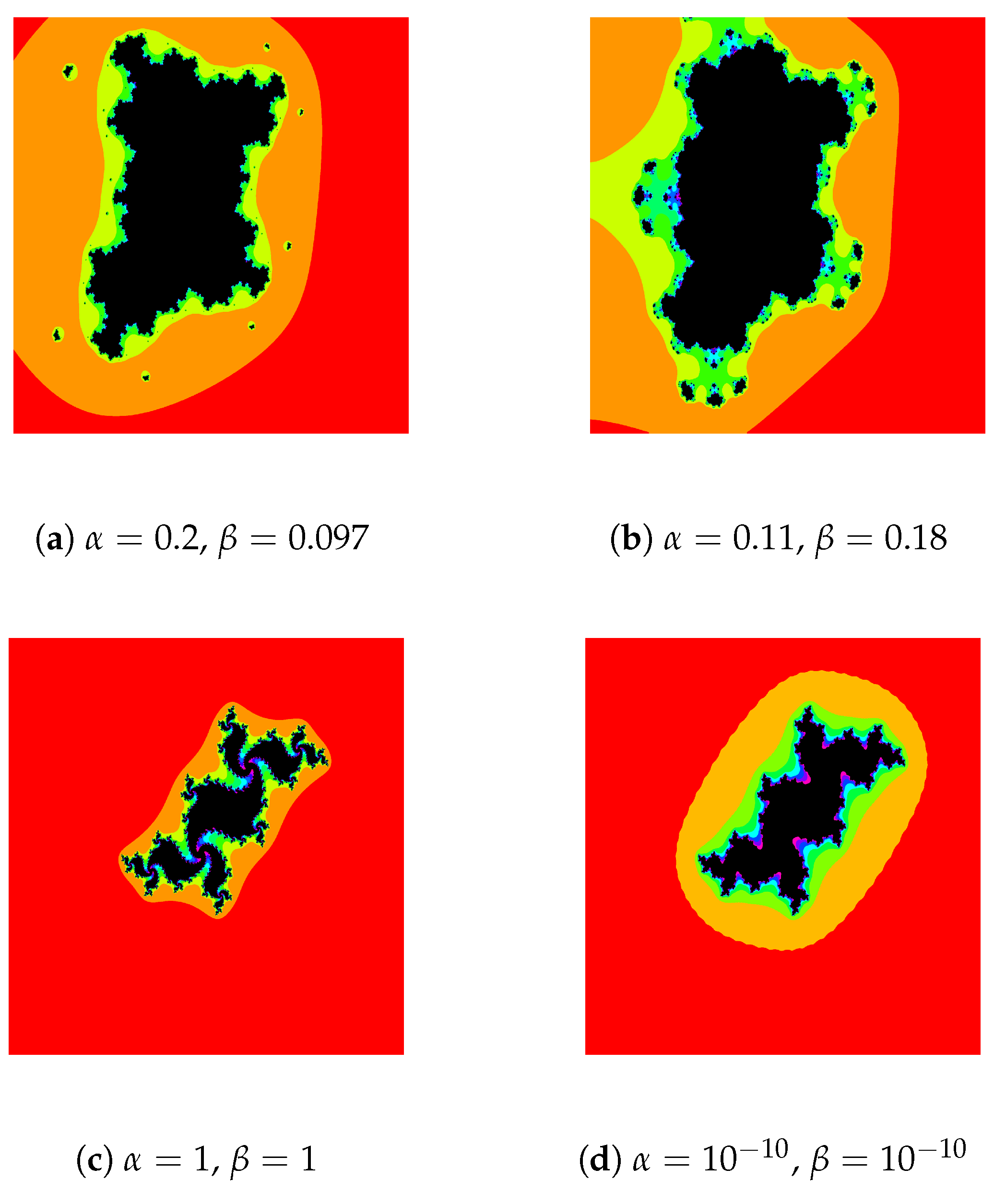
• For Figure 1, we consider the polynomial $T\left(x\right)=x^2+(-0.5+0.7i)x+(-0.01+0.18i)$ and $A=[-2.5,2.5]\times [-2.1,2.1]$. It is easy to see that T has one attracting fixed point, $p=-0.1427+0.1019i$. Observe that for $\alpha =0.2$, $\beta =0.097$ and $\alpha =0.11$,$\beta =0.18$ we obtain different images due to color variation caused by parameters. It is interesting to note that for $\alpha =1$, $\beta =1$ and $\alpha ={10}^{-10}$, $\beta ={10}^{-10}$ we have similar shapes but there is clear variation of colors.
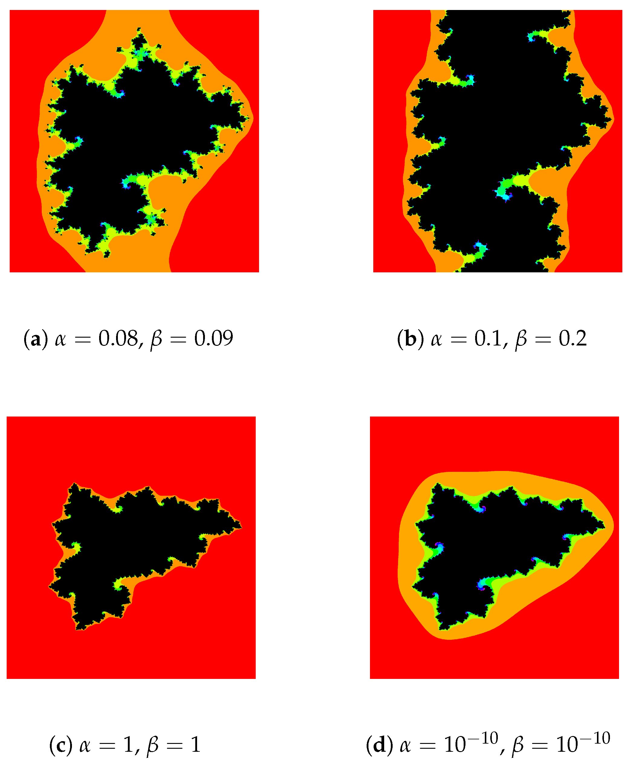
• For Figure 2, we consider the polynomial $T\left(x\right)=x^3+(-0.275+0.5i)x+(-0.559+0.35i)$ and $A=[-1.5,1.5]\times [-1.8,1.8]$. The polynomial T has attracting fixed point $p\sim -0.6434+0.2687i$ in A. Note that the cubic Julia sets for $\alpha =0.08$ and $\beta =0.09$ have more color variation as compared to the Julia sets for $\alpha =0.1$, and $\beta =0.2$. Again, for $\alpha =1$, $\beta =1$ and $\alpha ={10}^{-10}$, $\beta ={10}^{-10}$ the shapes are same but there is variability in colors.
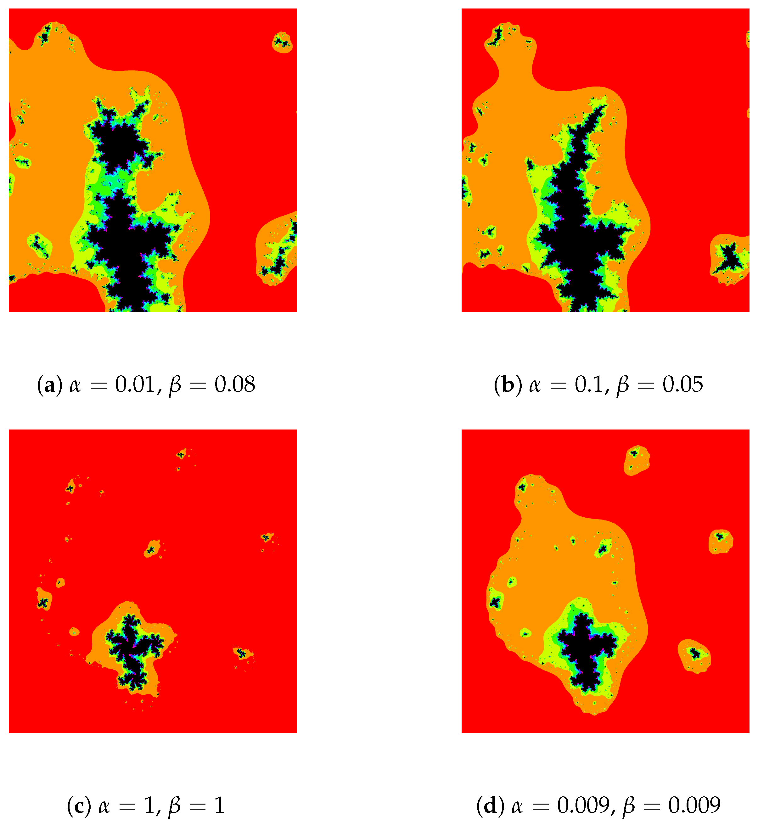
• For Figure 3, we input $T\left(x\right)=x^7+(0.23+1.2i)x+(0.5+0.7i)$ and $A={[-1.3,1.3]}^2$. The attracting fixed point of the polynomial is $p\sim -0.2391+0.5835i$. We can see that for $\alpha =0.01$ and $\beta =0.08$ the shape is spread and stretched while the shape is dense and neatly packed for $\alpha =0.1$ and $\beta =0.05$. Note the variation of colors in figures (C) and (D) as well.

3.2. Generation of Mandelbrot Sets

Following Algorithm 2 is the pseudocode for the generation of Mandelbrot sets. Note that $T^{\prime }\left(z\right)$ represents the iteration process.

Algorithm 2: Generation of Mandelbrot set.

For Figure 4 we input $A=[-2,2]\times [-1.2,2.5]$ and observe that for $\alpha =0.1$ and $\beta =0.3$, the shape is stretched and the bulb is wider and for $\alpha =0.75$ and $\beta =0.7$ the shape is compact with defined bulb. Notice the variation of colors for Mandelbrot sets for $\alpha =1$, $\beta =1$ and $\alpha =0.009$, $\beta =0.009$. Also, observe that Mandelbot sets generated are symmetric about origin.

4. Conclusions

In this paper, a Picard Ishikawa type orbit was used to study the behaviour of complex poylnomials. We obtained escape criterions for complex quadratic, cubic and higher degree polynomials. Some alluring Julia and Mandelbrot sets have been generated. We also observed that the variation of parameters has shown eminent changes in the Julia and Mandelbrot sets. Our results are different from comparable existing results as we obtain escape criterion and fractals for polynomials of the form $T\left(x\right)=x^n+mx+r$ where $m,r\in \mathbb{C}$ without using the Jungck iterative process. It is also worth mentioning that the behaviour of the polynomial and shape of the fractal generated under the iterative process (2) is different and unique as compared to the iterative process studied before in the literature [1,24,29,32].

References

1. Barnsley, M. Fractals Everywhere, 2nd ed.; Academic Press: San Diego, CA, USA, 1993. [Google Scholar]
2. Hundertmark-Zauôkovù, A. On the convergence of fixed point iterations for the moving geometry in a fluid-structure interaction problem. J. Differ. Equ. 2019, 267, 7002–7046. [Google Scholar] [CrossRef]
3. Rahmani, M.; Koutsopoulos, H.N.; Jenelius, E. Travel time estimation from sparse floating car data with consistent path inference: A fixed point approach. Transp. Res. Part C Emerg. Technol. 2017, 85, 628–643. [Google Scholar] [CrossRef]
4. Strogatz, S.H. Nonlinear Dynamics and Chaos With Applications to Physics, Biology, Chemistry, and Engineering, 2nd ed.; CRC Press: Boca Raton, FL, USA, 2018. [Google Scholar]
5. Julia, G. Memoire sur l’iteration des functions rationnelles. J. Math. Pures Appl. 1918, 8, 737–747. [Google Scholar]
6. Devaney, R.L. A First Course in Chaotic Dynamical Systems: Theory and Experiment, 2nd ed.; Addison-Wesley: Boston, MA, USA, 1992. [Google Scholar]
7. Falconer, K. Fractal Geometry: Mathematical Foundations and Applications, 2nd ed.; John Wiley & Sons: Chichester, UK, 2004. [Google Scholar]
8. Frame, M.; Robertson, J. A generalized Mandelbrot set and the role of critical points. Comput. Graph. 1992, 16, 35–40. [Google Scholar] [CrossRef]
9. Brouwer, L.E.J. Über Abbildungen von Mannigfaltigkeiten. Math. Ann. 1912, 71, 97–115. [Google Scholar] [CrossRef] [Green Version]
10. Mandelbrot, B.B. The Fractal Geometry of Nature; W.H. Freeman: New York, NY, USA, 1983; Volume 2. [Google Scholar]
11. Debnath, L. A brief historical introduction to fractals and fractal geometry. Int. J. Math. Educ. Sci. Technol. 2006, 37, 29–50. [Google Scholar] [CrossRef]
12. Lakhtakia, A.; Varadan, W.; Messier, R.; Varadan, V.K. On the symmetries of the Julia sets for the process zp + c. J. Phys. A Math. Gen. 1987, 20, 3533–3535. [Google Scholar] [CrossRef]
13. Negi, A.; Rani, M. Midgets of superior Mandelbrot set. Chaos Solitons Fract. 2008, 36, 237–245. [Google Scholar] [CrossRef]
14. Negi, A.; Rani, M. A new approach to dynamic noise on superior Mandelbrot set. Chaos Solitons Fract. 2008, 36, 1089–1096. [Google Scholar] [CrossRef]
15. Rochon, D. A generalized Mandelbrot set for bicomplex numbers. Fractals 2000, 8, 355–368. [Google Scholar] [CrossRef]
16. Wang, X.; Sun, Y. The general quaternionic M-J sets on the mapping zzα + c(α ∈ ℕ). Comput. Math. Appl. 2007, 53, 1718–1732. [Google Scholar] [CrossRef] [Green Version]
17. Rani, M. Theoretical Framework for Fractal Models under Two-Step Feedback Process. Ph.D. Thesis, Kumaun University, Nainital, India, 2016. [Google Scholar]
18. Rani, M.; Kumar, V. Superior Julia set. Res. Math. Educ. 2004, 8, 261–277. [Google Scholar]
19. Rani, M.; Kumar, V. Superior Mandelbrot set. Res. Math. Educ. 2004, 8, 279–291. [Google Scholar]
20. Rani, M.; Chauhan, Y.S.; Negi, A. Non linear dynamics of Ishikawa iteration. Int. J. Comput. Appl. 2010, 7, 43–49. [Google Scholar] [CrossRef]
21. Chauhan, Y.S.; Rana, R.; Negi, A. New Julia sets of Ishikawa iterates. Int. J. Comput. Appl. 2010, 7, 34–42. [Google Scholar] [CrossRef]
22. Chauhan, Y.S.; Rana, R.; Negi, A. Complex dynamics of Ishikawa iterates for non integer values. Int. J. Comput. Appl. 2010, 9, 9–16. [Google Scholar] [CrossRef]
23. Ashish; Rani, M.; Chugh, R. Julia sets and Mandelbrot sets in Noor orbit. Appl. Math. Comput. 2014, 228, 615–631. [Google Scholar]
24. Kang, S.M.; Rafiq, A.; Latif, A.; Shahid, A.A.; Ali, F. Fractals through modified iteration scheme. Filomat 2016, 30, 3033–3046. [Google Scholar] [CrossRef] [Green Version]
25. Kang, S.M.; Rafiq, A.; Latif, A.; Shahid, A.A.; Kwun, Y.C. Tricorns and multicorns of S-iteration scheme. J. Funct. Spaces 2015, 2015, 417167. [Google Scholar]
26. Kumari, M.; Ashish, R.C. New Julia and Mandelbrot sets for a new faster iterative process. Int. J. Pure Appl. Math. 2016, 107, 161–177. [Google Scholar] [CrossRef] [Green Version]
27. Kang, S.M.; Nazeer, W.; Tanveer, M.; Shahid, A.A. New fixed point results for fractal generation in Jungck Noor orbit with s-convexity. J. Funct. Spaces 2015, 2015, 963016. [Google Scholar] [CrossRef] [Green Version]
28. Kang, S.M.; Rafiq, A.; Tanveer, M.; Ali, F.; Kwun, Y.C. Julia and Mandelbrot sets in modified Jungck three-step orbit. Wulfenia J. 2015, 22, 167–185. [Google Scholar]
29. Kwun, Y.C.; Tanveer, M.; Nazeer, W.; Abbas, M.; Kang, S.M. Fractal generation in modified Jungck-S orbit. IEEE Access 2019, 7, 35060–35071. [Google Scholar] [CrossRef]
30. Proakis, J.G.; Manolakis, D.G. Digital Signal Processing: Principles, Algorithms and Applications, 4th ed.; Pearson: Bengaluru, India, 2007. [Google Scholar]
31. Mishra, M.K.; Ojha, D.B.; Sharma, D. Fixed point results in tricorn and multicorns of Ishikawa iteration and s-convexity. IJEST 2011, 2, 157–160. [Google Scholar]
32. Cho, S.Y.; Shahid, A.A.; Nazeer, W.; Kang, S.M. Fixed point results for fractal generation in noor orbit and s-convexity. SpringerPlus 2016, 5, 1843. [Google Scholar] [CrossRef] [PubMed] [Green Version]
33. Nazeer, W.; Kang, S.M.; Tanveer, M.; Shahid, A.A. Fixed point results in the generation of Julia and Mandelbrot sets. J. Inequal. Appl. 2015, 2015, 298. [Google Scholar] [CrossRef] [Green Version]
34. Piri, H.; Daraby, B.; Rahrovi, S.; Ghasemi, M. Approximating fixed points of generalized α-nonexpansive mappings Banach spaces by new faster iteration process. Numer. Algorithms 2018, 81, 1129–1148. [Google Scholar] [CrossRef]
Figure 1. Quadratic Julia sets.
Symmetry 12 00086 g001
Figure 2. Cubic Julia sets.
Symmetry 12 00086 g002
Figure 3. Septic Julia sets.
Symmetry 12 00086 g003
Figure 4. Mandelbrot sets.
Symmetry 12 00086 g004