Evaluation of Rolling Bearing Performance Degradation Using Wavelet Packet Energy Entropy and RBF Neural Network

Abstract

Rolling bearings are the most important parts in rotating machinery, and one of the most vulnerable parts to failure. The rolling bearing is a cyclic symmetrical structure that is stable under normal operating conditions. However, when the rolling bearing fails, its symmetry is destroyed, resulting in unstable performance and causing major accidents. If the performance of rolling bearings can be monitored and evaluated in real time, maintenance strategies can be implemented promptly. In this paper, by using wavelet packet energy entropy (WPEE), the early fault-free features of bearing and the failure samples of similar bearings are decomposed firstly, and the energy value is extracted as the original feature, simultaneously. Secondly, a radial basis function (RBF) neural network model is established by using early fault-free features and similar bearing failure characteristics. The bearing full-life data characteristics of the extracted features are added into the RBF model in an iterative manner to obtain performance degradation Indicator. Boxplot was introduced as an adaptive threshold method to determine the failure threshold. Finally, the results are verified by empirical mode decomposition and Hilbert envelope demodulation. A bearing accelerated life experiment is performed to validate the feasibility and validity of the proposed method. The experimental results show that the method can diagnose early fault points in time and evaluate the degree of bearing degradation, which is of great significance for industrial practical applications.

1. Introduction

Rolling bearing, as an important part of rotating machinery, plays a key role in the stable and safe operation of mechanical equipment. Therefore, real-time monitoring and performance degradation evaluation of rolling bearings are of great significance [1]. In general, damage to rolling bearings requires a process covering shifts from normal to degraded to failure. If the bearing can be quantitatively evaluated during the degradation process, major industrial losses caused by bearing failure can largely be avoided with timely targeted planning for the maintenance of the equipment [2].

The evaluation basis of bearing faults includes vibration signals [3], temperature changes [4], etc., while the most important part is the study of vibration signals. Bearing defects main sources of bearing-induced vibration in the bearing components. Defect identification has great influence on real-time monitoring systems [5]. Bearing defects can be classified as distributed and localized defects. Distributed defects, such as misaligned races, surface roughness, and waviness, are caused by the improper installation or manufacturing process [6]. It may lead to out-of-balance rotations of the spindle, which contribute significantly to the vibration of the spindle in many cases. Localized defects, such as cracks, pits, and spalls, are caused by fatigue damage on the rolling surfaces [7]. In addition, the vibration of the bearing also has interferences such as natural frequency and resonance phenomenon, which will be the content of bearing failure research.

In recent years, many researchers have carried out a lot of exploratory research on the feature extraction and performance degradation evaluation of rolling bearings. Chen et al. used information entropy theory to extract the performance degradation index (DI) sequence of bearing signals. Then the least square support vector machine (LS-SVM) is used to perform regression prediction on the extracted features, and accurate prediction results are obtained, which has strong practicability [8]. Soualhi et al. used empirical mode decomposition (EMD) to decompose the signal and extract the spectral amplitude corresponding to the characteristic frequency of the rolling bearing fault to form the eigenvector, and construct the rolling bearing fault DI through a support vector machine (SVM) [9]. Cheng et al. proposed the limited feature select sample (LFSS) algorithm for the feature selection problem of performance degradation assessment. The root mean square value and the 3$\sigma$ rule were used to judge the initial point of fault to determine the feature selection sample [10]. Brkovic et al. perform early fault detection on bearings in the energy system. The normalized vibration signal is wavelet transformed, and the logarithmic energy entropy and standard deviation are extracted as features. Finally, the secondary classifier is used for fault detection and diagnosis. This technical result is applied in the actual production environment [11]. In addition, methods for processing bearing vibration signals include time domain analysis [12], frequency domain analysis [13], and variational mode decomposition [14]. The above methods have achieved good results in the evaluation of bearing performance degradation, but there are still some problems. For example, information entropy can reflect the nonlinearity of the signal, but cannot handle non-stationary information very well. EMD decomposition signals are prone to modal aliasing. The LFSS algorithm selects the feature samples to use 3$\sigma$ and the samples need to follow the normal distribution. The traditional time domain and frequency domain analysis considers the vibration signal as a stationary signal processing, and has drawbacks such as insufficient representation of the bearing characteristics of the bearing and insufficient evaluation capability. Although the variational mode decomposition (VMD) can solve the EMD modal aliasing problem, it needs to use the optimization algorithm to select the preset scale and the penalty factor, which increases the complexity and difficulty of the operation.

In this paper, by combining the features of wavelet packet decomposition and information entropy, wavelet packet energy entropy (WPEE) is proposed as the feature extraction method. This method can not only highlight the good resolution of wavelet packet decomposition for non-stationary signal feature analysis, but also process nonlinear signal with information entropy. Wan et al. used the wavelet packet transform as the band decomposition method of the bearing vibration signal, and proposed the Teager energy entropy ratio as the calculation index of the wavelet bun zone. WPT replaced the traditional filter to more clearly divide the frequency band while suppressing noise interference. The TEER is used as the calculation index of the wavelet sub-band, the impact characteristics and periodic characteristics can be adaptively reflected [15]. Ma et al. combine wavelet packet transform with information entropy, and propose a fault diagnosis method based on wavelet packet energy entropy (WPEE) and fuzzy limit learning machine. The method uses the WPEE method to extract sensitive and transient features in massive data, and improves the recognition accuracy and reliability of subsequent classification models [16]. Li et al. proposed an improved WPEE and GA-SVM (Genetic Algorithm optimization support vector machine) combination to overcome the difficulty in accurately extracting feature vectors in bearing fault diagnosis. The improved WPEE method is applied to the fault feature extraction of rolling bearings, and compared with the unmodified wavelet packet feature extraction method. The results show that the improved WPEE processed signal can better characterize the fault characteristics [17]. Research literature and experimental analysis shows that the combination of wavelet packet transform and energy entropy can more fully reflect the detailed information of a fault signal.

Early fault diagnosis based on artificial intelligence (AI) as an effective solution for emerging industrial applications and fault identification is receiving more and more attention from academic and industrial circles [18]. The early fault diagnosis method based on AI, by machine learning technology, which can effectively overcome the limitation that researchers require rich professional knowledge. In early fault diagnosis schemes by AI-based, the most commonly used models are Support Vector Data Description (SVDD) [19], Support Vector Machine (SVM) [20], Gauss Mixture Model (GMM) [21], and Artificial Neural Network (ANN) [22].

As an artificial intelligence model, ANN is widely used in pattern recognition, prediction and estimation, automatic control, industrial modeling and other fields [23]. Durodola proposed an artificial neural network approach that included the effects of mean stress in the frequency domain method to predict fatigue damage. The results show that the method can predict fatigue damage including the influence of average stress. Compared with other methods, neural network method has higher resolution [24]. Al-Abdullah used artificial neural network method to establish a suitable force and temperature model based on real experimental measurement data of cancellous artificial tissue bone milling. The calculation results are in good agreement with the experimental results. The model can be used to optimize the real-time bone milling control [25]. It can be seen that neural network is powerful and has obvious advantages. In the evaluation of bearing performance degradation, the neural network mainly uses the strong nonlinearity of ANN to establish the relationship between the characteristics and the bearing state, and then evaluates the degradation state of the bearing. Hong et al. used self-organizing map neural network (SOM) to evaluate the health status of rolling bearings, by training SOM with data in the non-fault state, and obtain health monitoring values from the data under test [26]. Chen et al. carried on the principal component analysis to generate features as an input into the SOM neural network, and then carried on the fault diagnosis and the performance degradation appraisal to the bearing [27]. Liu et al. used the firefly optimization algorithm to obtain the optimal initial weight and threshold of BP neural network, and used the optimized BP neural network to evaluate the degree of bearing performance degradation [28]. However, the back propagation (BP) neural network has problems such as local minimization and different network structure selection. The SOM algorithm converges slowly and the network size is difficult to determine. RBF neural network is widely used in industrial and intelligent diagnostic system fields because of its strong generalization ability, fast convergence speed, good global convergence, and simple structure. Arnaiz used neural networks as an analytical tool for predicting tool deflection errors. Two types of neural networks, multilayer perceptron (MLP) and RBF, were tested. The results indicate that RBF has a good advantage in the training and tuning time of the model [29]. Mahmoud et al. combined the RBF neural network with the fuzzy logic system for the fault detection of photovoltaic systems and achieved good results [30]. Zhao et al. used RBF neural network in bearing fault diagnosis. The S-transform and Singular Value Decomposition (SVD) theory were used to process the vibration signal. Zhao et al. then trained an RBF neural network for pattern recognition and fault diagnosis [31]. The existing article used the RBF neural network for qualitative identification of failure modes and did not involve quantitative assessment of the degree of failure or degree of performance degradation. Therefore, the RBF neural network is used in our analysis of the rolling bearing fatigue test to quantitatively analyze the degradation state of bearing performance.

To this end, this paper proposes a combination of WPEE and RBF neural network performance degradation assessment method. In light of the advantages of WPEE in dealing with vibration signals, an RBF neural network is applied to quantitatively evaluate the performance degradation. In this paper, the feature of rolling bearing data is extracted by WPEE. The model of the RBF neural network, by using early faultless samples and similar bearing failure samples, is established, and the bearing life test data is input into the model through iterative methods to obtain the performance degradation evaluation curve, which is established as the threshold curve. The box plot is calculated based on the actual existing data. The curve can be adjusted adaptively, and the early fault point of the bearing is determined according to the intersection of the threshold curve and the performance degradation evaluation curve. In the experimental part, the discrete seeded fault bearing test data was used first to verify the ability to distinguish the bearing faults of different sizes, and then the feasibility of the method was tested with the whole life test data of bearings that were obtained from healthy operation to failure. Three RBF neural network models with different radial basis functions were selected for the performance degradation evaluation curve, and the optimal Gaussian basis function was selected as the radial basis function to act as a comparison. The performance degradation assessment curve is made by using the commonly used monitoring indicators, which is compared with the proposed method, to highlight the superiority of the proposed method. Finally, the envelope demodulation is used to verify the accuracy of the experimental results, and the rolling bearing accelerated fatigue life test is conducted to verify the feasibility of the method.

2. Backgrounds

2.1. Wavelet Packet Energy Entropy

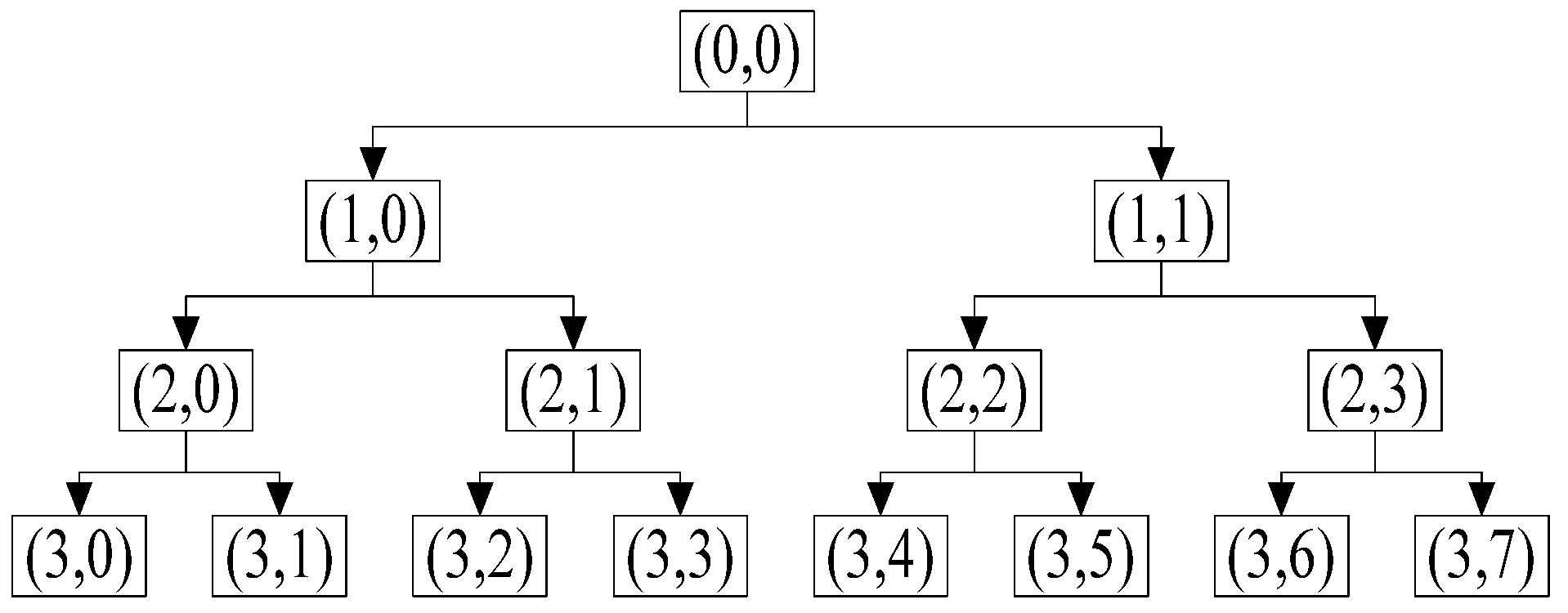
2.1.1. Wavelet Packet Decomposition Layers and Selection of Wavelet Basis

Wavelet packet transform is a technique of time-frequency analysis that automatically selects the frequency band range and completes the band matching [32]. As a mathematical tool for processing non-stationary signals, wavelet packet transform is widely used in signal processing.

Wavelet function definition: Let $\psi \left(t\right)$ be a square integrable function if its Fourier transform $\psi \left(\omega \right)$ satisfies:

$$C_{\psi }={\displaystyle {\int }_R\frac{\left|\psi \left(\omega \right)\right|}{\left|\omega \right|}}d\omega <\infty$$

(1)

where $\psi \left(t\right)$ is called a basic wavelet.

Wavelet analysis is a time-frequency localization analysis method that can change the time window and frequency window. The signal is decomposed into components located in different frequency bands and time periods, which not only can decompose the low frequency part of the signal, but also effectively decompose the high frequency of the signal. By decomposing and reconstructing the signal in different scales, wavelet analysis can obtain detailed information about the distribution of the original signal in different frequency bands. The tree structure diagram of the 3-layer wavelet packet decomposition is shown in Figure 1. The wavelet packet decomposition coefficient reconstruction can extract 8 sub-bands of the wavelet packet energy from the low frequency to the high frequency.

Choosing an appropriate wavelet basis function can more accurately highlight the characteristics of the signal, which has a decisive effect on the evaluation results of the model. In this paper, the wavelet basis function Daubechies 5 is selected, and its time domain waveform is similar to the rolling bearing vibration signal waveform, which can accurately reflect the prominent points of the fault signal. The increase of the number of decomposition layers can more accurately depict the vibration signal. Therefore 3-layer wavelet packet decomposition method is selected in this paper.

2.1.2. Wavelet Packet Energy Entropy Feature Extraction

The basic idea of the WPEE is to decompose the vibration signal through the wavelet packet, obtain the decomposition coefficient, reconstruct the coefficient, and calculate the energy of the reconstruction coefficient feature, then to find the ratio of the energy of each node to the total energy. Finally, the information entropy of the feature energy ratio is obtained. This process gives an evaluation measure of the complexity of the vibration signal.

The information entropy calculation formula is as shown in Equation (2):

$$S_i=-g_i{\log }_2{g}_i$$

(2)

where $S_i$ is the energy entropy of the $ith$ wavelet packet node and $g_i$ is the energy ratio of the $ith$ wavelet packet node.

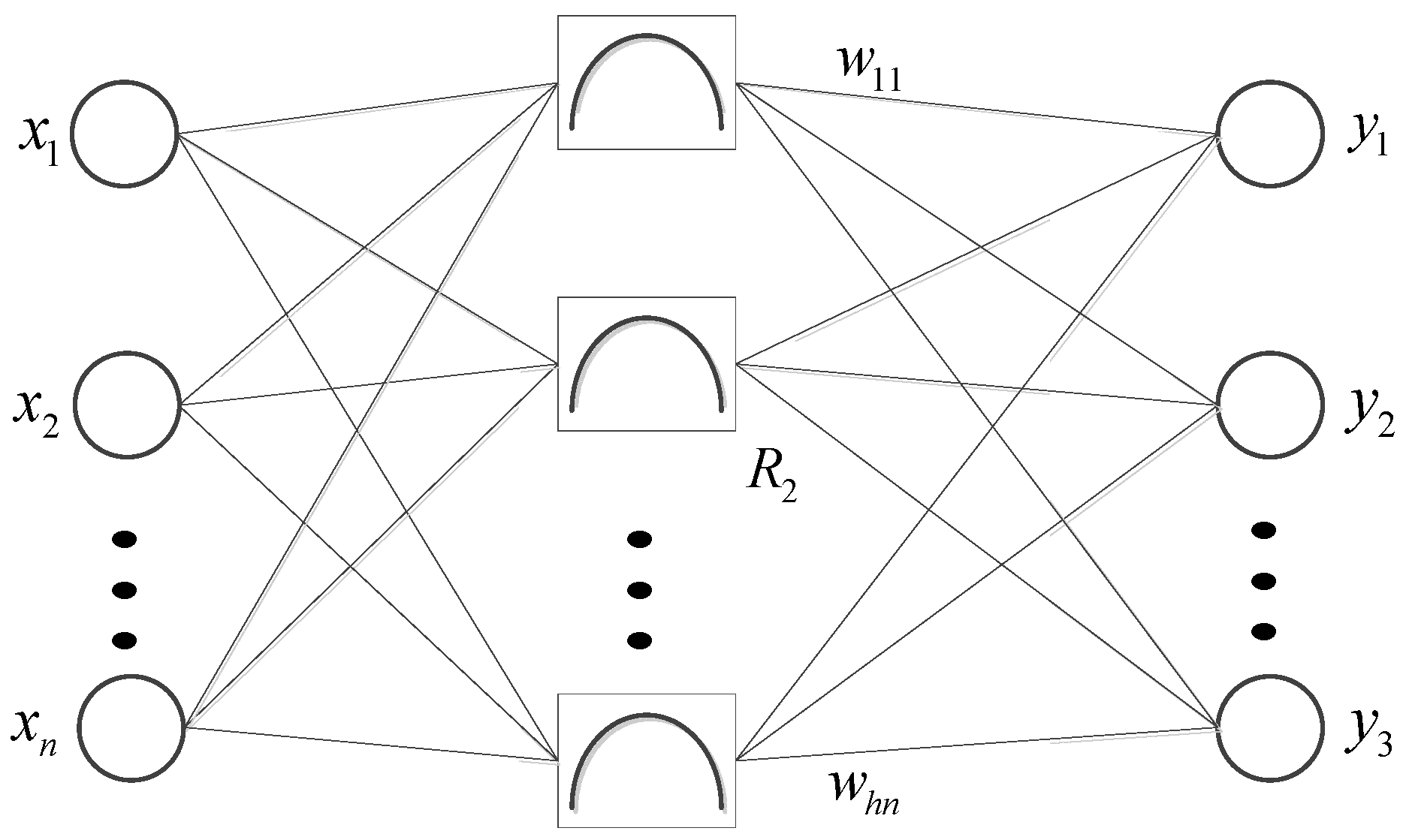
2.2. RBF Neural Network Model

The RBF neural network is a single hidden layer structure and is one of the most important neural network models [33]. RBF neural network is a kind of forward neural network with good performance. It has the advantages of a simple network structure, fast convergence speed, excellent approximation performance, and no local minimum problem. The functions of the hidden layer nodes are generally non-linear. In general, the number of hidden layer neurons is sufficient, and the RBF neural network can approximate any single-valued continuous function with arbitrary precision.

The basic idea of RBF neural network is to use radial basis function as node activation function of hidden layer and map input vector to hidden space, so that the low-dimensional linear non-separable data of input layer can be mapped to the high-dimensional data of output layer, and the data can be linearly separable in high-dimensional space [34]. The topology of the RBF network is shown in Figure 2.

The Gauss function is usually selected as the radial basis function, as shown in Equation (3):

$$h_j\left(x\right)=\exp ((-\frac{1}{r_j{}^2}){\Vert x-c_j\Vert }^2)$$

(3)

For the convenience of comparison, Reflected Sigmoidal function and Inverse Multiquadrics function are also selected as radial basis functions, and their formulas as shown in Equations (4) and (5), respectively.

$$h_j\left(x\right)=\frac{1}{1+\exp ((-\frac{1}{r_j{}^2}){\Vert x-c_j\Vert }^2)}$$

(4)

$$h_j(x)=\frac{1}{{({\Vert x-c_j\Vert }^2+r_j{}^2)}^{1/2}}$$

(5)

where $h_j\left(x\right)$ is the output of the $jth$ RBF node; $c_j$ and $r_j$ are the center value and width of the $jth$ RBF node, respectively.

The output layer of the RBF neural network is a linear output, as shown in Equation (6):

$$y_k={\displaystyle \sum _{j=1}^m{w}_{kj}{h}_j(x)}{+\mathrm{b}}_k$$

(6)

where $y_k(x)$ is the $kth$ output of the network for the input vector $x$;$m$ is the number of hidden nodes; $w_{kj}$ is the connection weight of the $kth$ output node and the $jth$ hidden node, and $b_k$ is the off set, $j=1,2,\cdots m$.

The training data of the extracted WPEE is adopted to train the RBF neural network model. The classification results are two different types, so the number of hidden nodes is set as 2 and the overlap coefficient of hidden nodes is set as 1.0. The target tag was set, with the fault-free sample as 0 and the failure sample of similar bearing as 1. The classification center was saved through Gaussian kernel function classification. The bearing life test data is taken as the test sample, and the characteristics are extracted and input into the model. The model calculates the Euclidean distance from the sample to the classification center, input to Formula (6), the output vector is calculated.

2.3. Adaptive Threshold Setting

A box-plot consists of five statistics in the data: upper limit (Maximum value in non-abnormal range), upper quartile, median, lower quartile and lower bound (Minimum value in non-abnormal range). It is a method for describing data, which can be used to identify data outliers, compare the shapes of several batches of data, and so on. As shown in Figure 3. Hua et al. use box plots to identify abnormal conditions in the ethylene production process [35]. Liu et al. used box plots to denoise the original signal of the bearing [36]. This paper uses it as an adaptive threshold to determine the data outliers. The abnormality data in the bearing life is identified by the data of the performance degradation index, and the fault diagnosis is performed.

The basic principle of box plot analysis is to arrange the data from small to large and calculate the quartile of the data. Calculate the anomaly of the data by quartiles:

$$K\le L_1-1.5(L_3-L_1)$$

(7)

$$K\ge L_3+1.5(L_3-L_1)$$

(8)

where $K$ is an outlier, that is, the data is in an abnormal state; $L_1$ is the upper quartile; $L_3$ is the lower quartile.

The drawing of the box plot is based on the actual data to calculate the quartiles. Box plots are somewhat different from the classic way of identifying outliers. Classical methods such as the 3σ rule or the Z-score method based on normal distribution presuppose that the assumed data obeys the normal distribution, but the actual data often does not strictly obey the normal distribution, so the validity of the abnormal data is limited. The drawing of the box plot depends on the actual data. It is not necessary to assume that the data is subject to a specific distribution form, and there is no restriction on the data, so that the original shape of the data shape can be expressed visually and intuitively. Up to a quarter of the data can be moved away from normal data without affecting the quartile to a large extent, so outliers do not affect the drawing criteria of the box plot, the effect of identifying outliers is more objective. In summary, the box plot has certain advantages in judging data outliers. Therefore, this paper selects the box plot as the abnormal data identification method, and selects the maximum value of the box plot as the adaptive alarm threshold for performance degradation assessment.

The box-plot diagram is introduced as a method for setting the adaptive alarm threshold for performance degradation evaluation of rolling bearings. If there are consecutive multiple evaluation index values exceeding the abnormality of the box plot defined by the evaluation index value, it indicates that the performance degradation state of the bearing has undergone a large change. At the same time, an adaptive alarm line that changes with time can be obtained according to the constant change of the DI value.

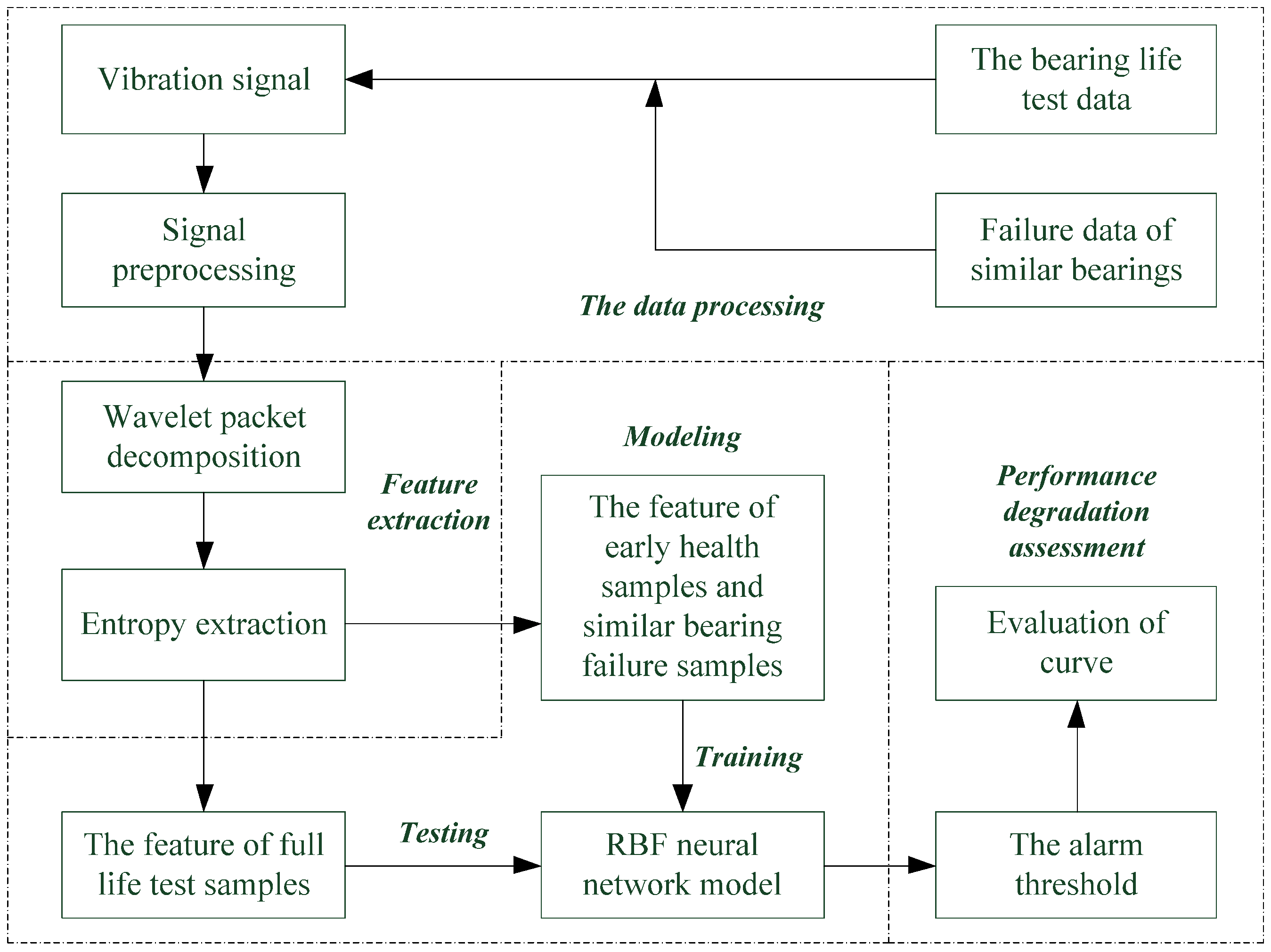
3. Establishment of Performance Degradation Assessment Model

The main steps of the rolling bearing performance degradation assessment model are as follows:

Step 1:

Perform wavelet packet decomposition on the rolling bearing vibration signal $X(\mathrm{t})$, and obtain all sub-band decomposition coefficients, a total of 8;

Step 2:

Step 2: Reconstruct the wavelet packet decomposition coefficients:

$$a_{j,k}(i)={\displaystyle \sum _n{a}_{j-1,k}(n)p_{i-2n}}+{\displaystyle \sum _n{b}_{j+1,k}(n)q_{i-2n}}$$

(9)

where $k=0,1,2,\cdots ,8$; $a_{0,k}=x(i)$,$i=0,1,2,\cdots ,N;1;N$ is the number of sampling points of the vibration signal; $x(i)$ is the discrete time domain signal; $j$ is the number of decomposition layers; $p\left(n\right)$ and $q\left(n\right)$ is the impulse response of the conjugate image filter $P$ and $Q$; $a_{j,k}(i)$ and $b_{j,k}(i)$ are the low frequency and high frequency decomposition coefficients, respectively.

Step 3:

The energy value of the last wavelet packet reconstruction coefficient $a_{3,k}(i)$ was obtained. Calculate the total energy of wavelet decomposition. Finally, the energy ratios of each wavelet packet node are obtained:

$$g_i=e_i/{\displaystyle \sum _{i=1}^8{e}_i}$$

(10)

where $e_i$ is the energy of the $ith$ wavelet packet node.

Thus, the wavelet packet energy ratio of the original signal is obtained, which is expressed as $G=[g_1,g_2,\cdots ,g_8]$. Finally, the energy entropy of the wavelet packet node is calculated by Equation (2):

Step 4:

Extracting the WPEE as the input eigenvector, and the RBF neural network model is established by using the early faultless samples and the failed samples of similar bearings. The model classifies all samples by using Euclidean distance, and obtains the cluster centers of the faultless samples and the failed samples, respectively.

Step 5:

Keep the model unchanged, and input the WPEE feature of the full-life bearing test data into the trained model through iterative method to obtain the model output value. According to the theory of the model, the output value of the model is the performance degradation evaluation index.

Step 6:

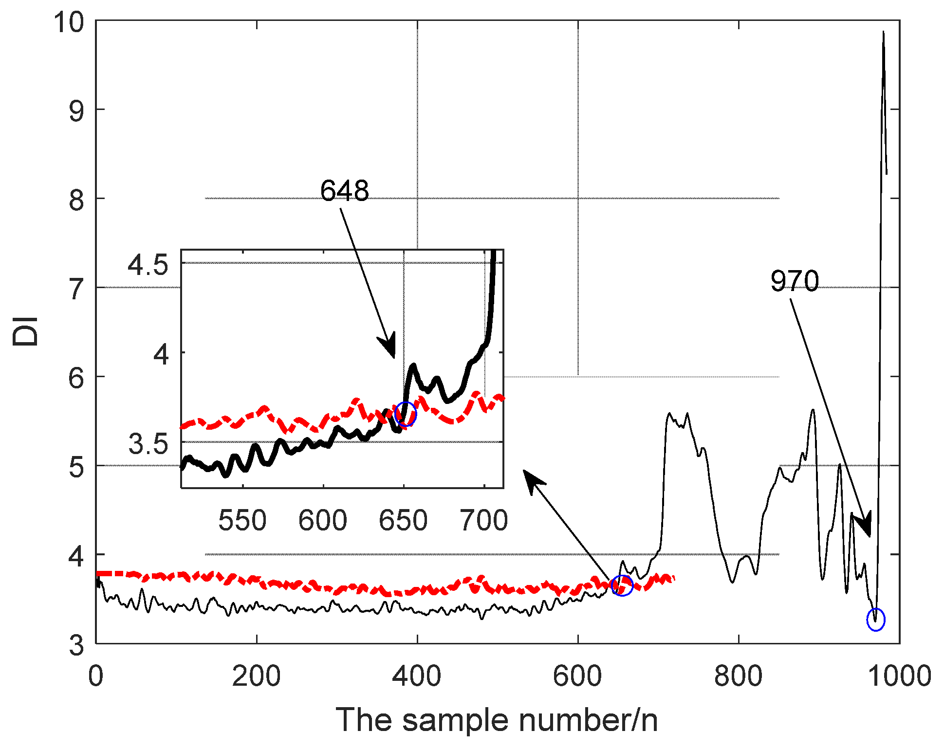
Calculate adaptive threshold curves, identify early failure points, and perform quantitative assessments.

The RBF neural network performance degradation assessment model is shown in Figure 4.

4. Experiment and Result Analysis

4.1. Bearing Discrete Data Verification

The QPZZ-II fault simulation test bench is adopted to conduct the experiment. It is mainly composed of variable speed drive motor, main shaft, biasing turntable, governor, gear box and bearings. The spindle is driven by the drive motor through the belt, the drive power is 0.55 KW, and the bearing is mounted on the right side of the spindle. Figure 5 shows the test bench and the acquisition device.

Faults with a width of 0.05 mm, 1.0 mm and 1.5 mm were processed on the outer rings of the three bearings by using electric sparks to simulate varying degrees of damage. Among them, three kinds of damage of different degrees are degree one, degree two and degree three.

The specific parameters of the test bench experiment are shown in

Table 1. Test bench parameters.

Type	Parameter
data acquisition card	NI-USB4431
sensor	DH107 piezoelectric sensor
motor speed	1218 rpm
load	80 kg
sample frequency	12,000 Hz
sample length	1024
bearing designation	N205EM
bearing bore diameter	25 mm
bearing outer diameter	52 mm
number of rolls	9

.

The time domain signal and spectrum of the samples under normal samples and different fault sizes of the rolling bearing are shown in Figure 6. As can be seen in the figure, the time domain and frequency spectrum under the normal signal and the degree one fault signal are different, but it is not obvious and can be ignored. Similarly, the spectral difference between the degree two and degree three fault spectra is small. Therefore, the size of the fault increases, the extent of the fault cannot be distinguished by the time domain signal and the spectrogram.

Establish a model of discrete data. 40 sets of normal samples and three levels of fault samples were selected as training samples. The number of test samples collected in the experiment is 10 groups in each state. The WPEE features of the normal sample and the three outer ring fault samples are extracted.

It can be seen in Figure 7 that the RBF evaluation value increases in a trapezoidal shape and the model test results are effective. Normal samples, degree one, degree two and degree three of sample can be significantly distinguished, and the evaluation values of normal samples and fault samples at all levels are well classified.

Discrete data is calculated using the root mean square value. The results obtained are shown in Figure 8.

It can be seen from Figure 8 that the RMS value of the sample is poorly differentiated in different states. And with the increase of the fault size, the RMS value has no obvious distinguishing effect. Especially in the faulty data, the result of the RMS value keeps fluctuating back and forth in a certain interval, and the discrimination effect is poor. Therefore, it has been successfully verified that the combination of WPEE and RBF neural network has a good effect on the degradation state of rolling bearing performance degradation.

4.2. Bearing Full Life Data Experimental Verification

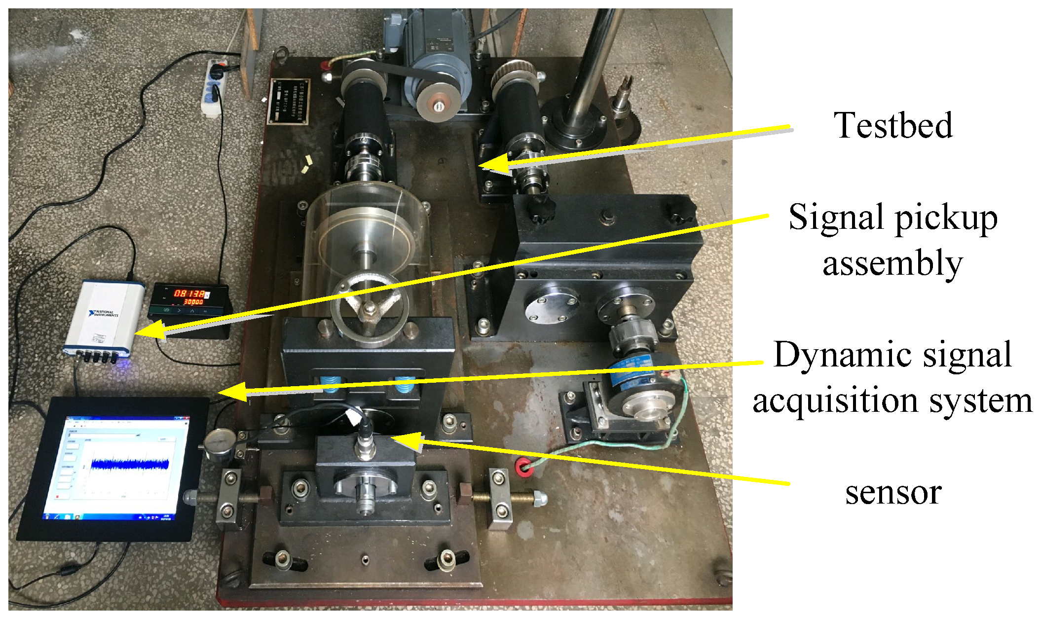
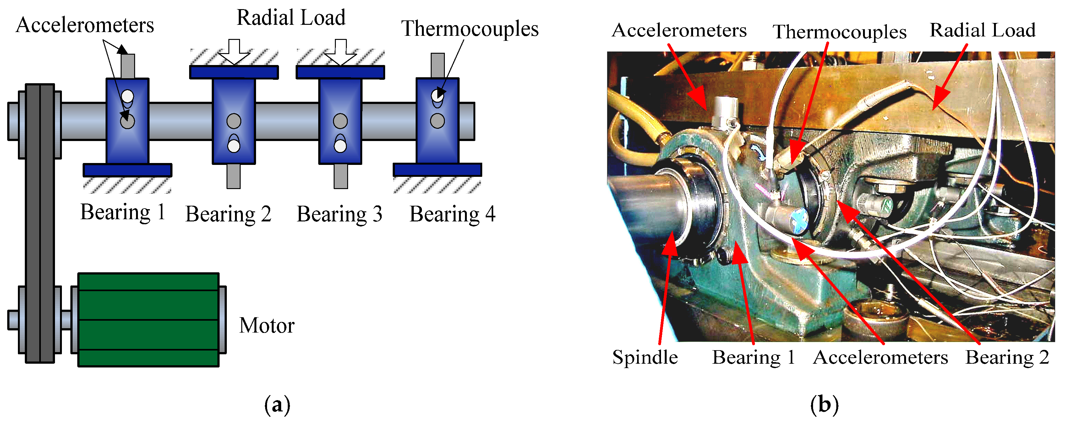
4.2.1. Test Bench Introduction

The experimental data which was collected by using the bearing fatigue life test bench is obtained from the Intelligent Maintenance System Center of the University of Cincinnati, USA [37]. The test bench is shown in Figure 9:

The test bench spindle is equipped with four double row roller Rexnord ZA-2115 bearings. The radial load of the bearing is approximately 2721.6 kg. The rotational speed is 2000 RPM. The data is collected interval 10 min with the NI DAQ-6062E data acquisition card. The sampling frequency is 20 kHz. Each data set consists of individual files that are vibration signal snapshots recorded of 1-s and each file consists of 20,480 points. Two acceleration sensors PCB353B33 were mounted on the cover of the bearing in the horizontal and vertical positions respectively. The oil circulation system is used to adjust the flow rate and temperature parameters of the lubricating oil. The magnetic plug is mounted inside the conduit of the feedback oil. Three sets of data were obtained in the experiment. In this paper, a total of 984 samples of the second set of data were used for performance degradation evaluation. Since there is no bearing failure data in the real-time monitoring, the failure data of similar bearing is used as the training sample. The failure of the third set of bearings and the failure of the second set of bearings are both outer ring failures. Therefore, the last 10 samples of the third set of failed bearings are selected as training samples. Since the vibration signals of the last two samples of the bearing were abnormal, the total number of samples was 982. By calculation, the outer ring fault characteristic frequency of the bearing is 236 Hz.

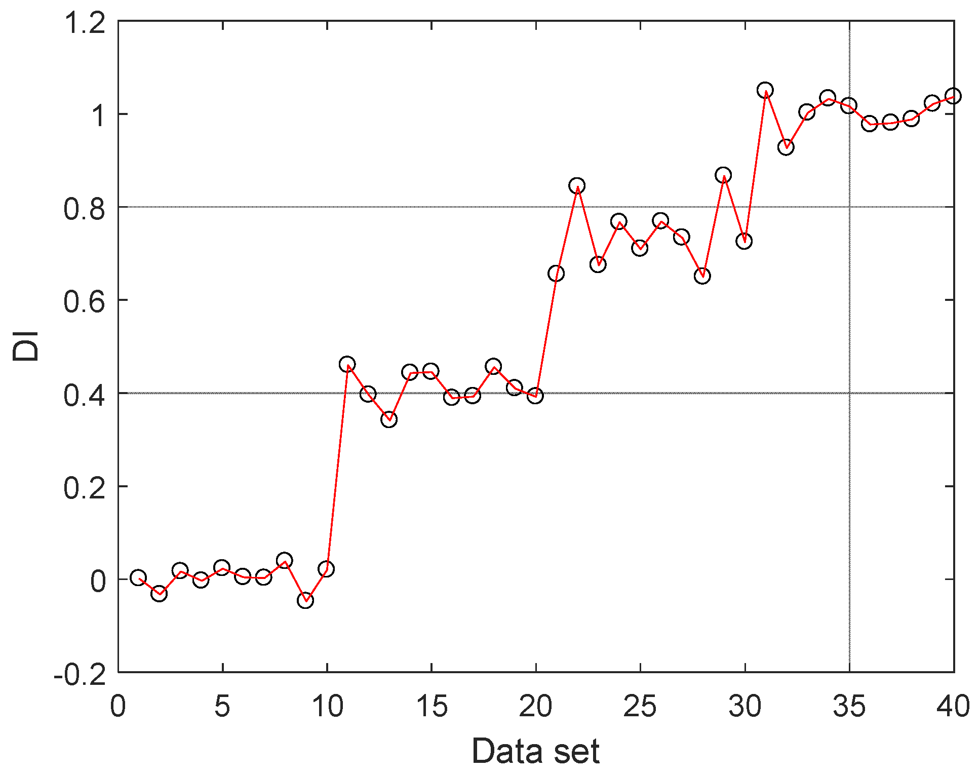
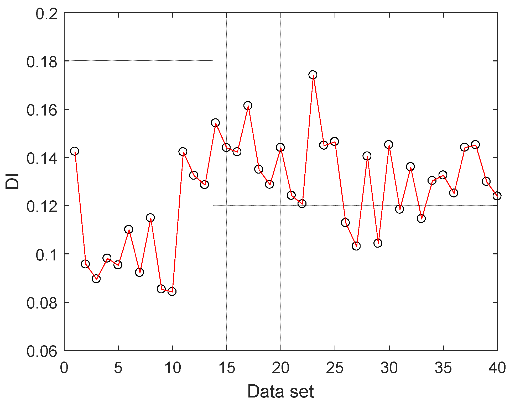
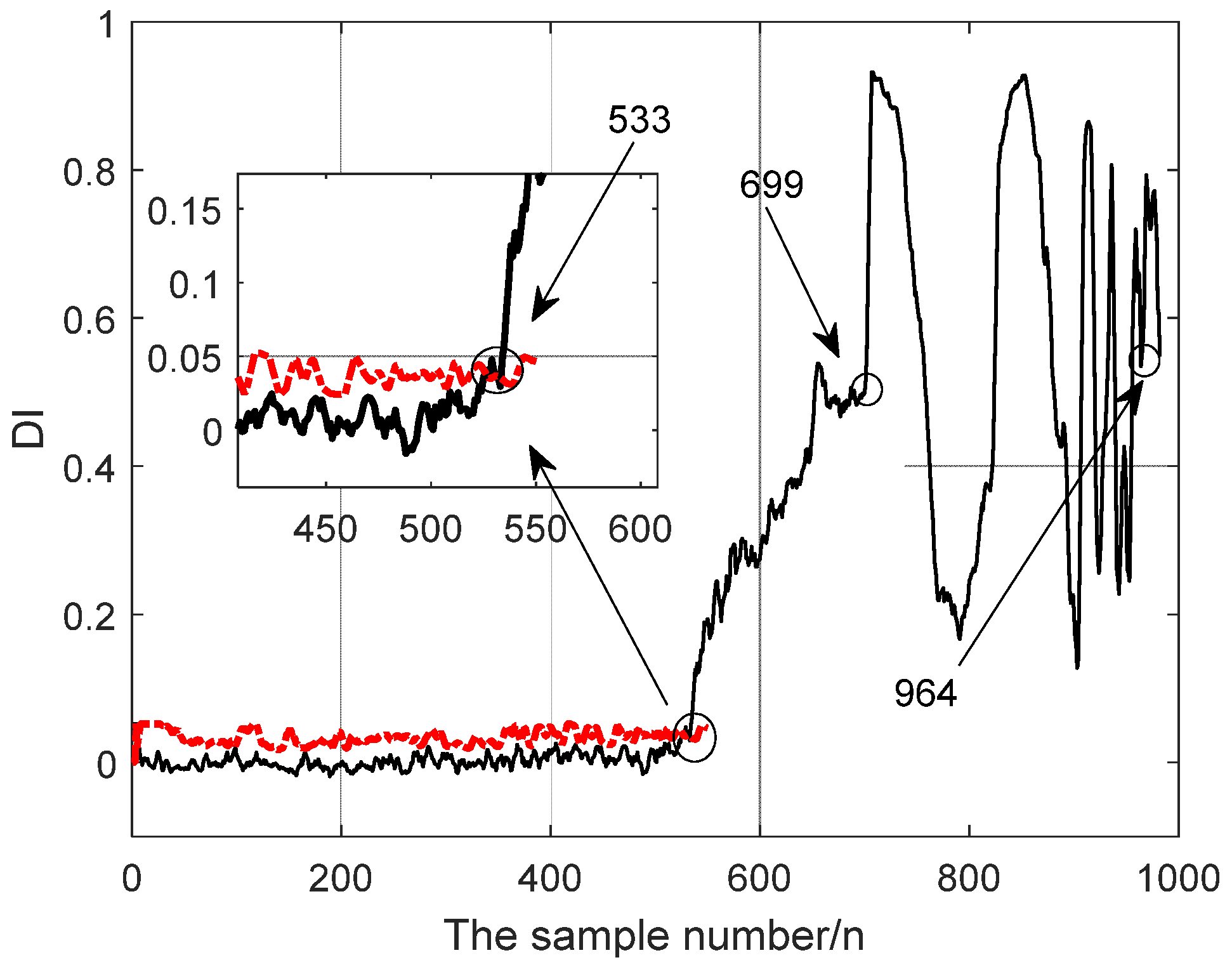
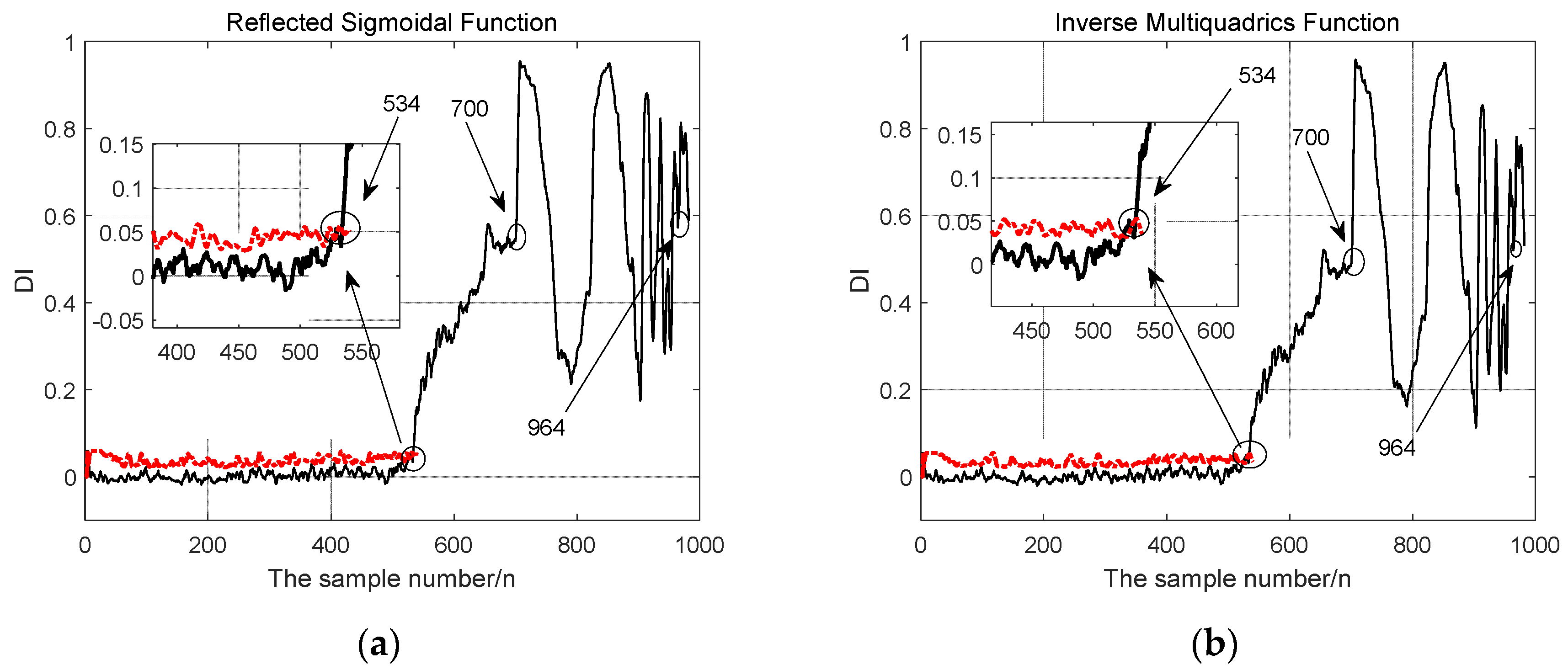
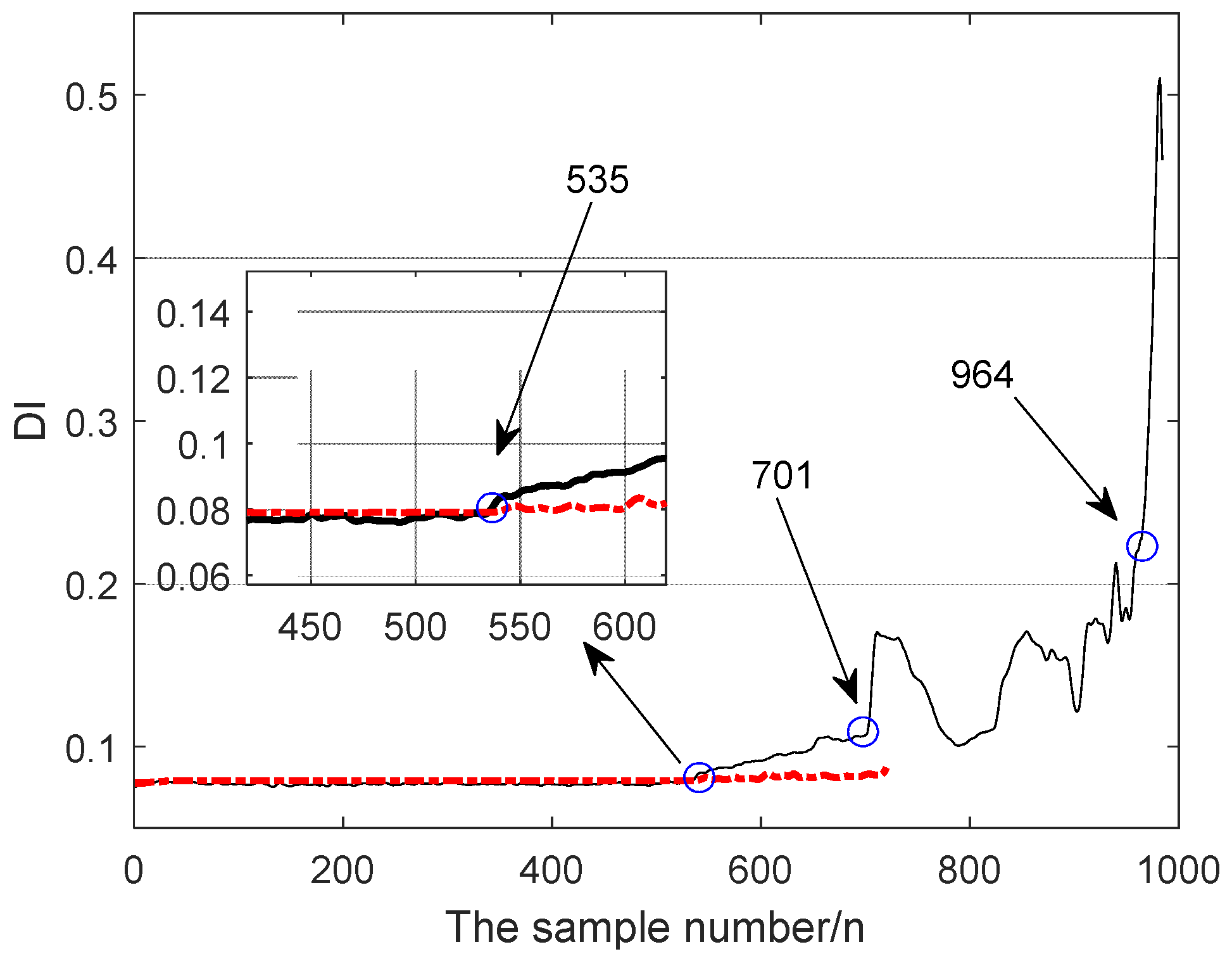
4.2.2. RBF Neural Network Model Evaluation Results

The first 100 sample of early fault-free data and the last 10 samples of failure data in the life-time data are selected as samples, and the features are extracted by WPEE, and a 110 × 8 input matrix is constructed, input the RBF model, and the model is trained to obtain the cluster center. After obtaining the performance degradation evaluation model, the 982 sets of full-life data are taken as samples, and the features are extracted. A test sample matrix of 982 × 8 is constructed and input into the model through iterative method to obtain the DI value in the bearing life cycle. After smoothing it, the performance degradation state is obtained as shown in Figure 10. In the following result analysis, the red curve is the threshold curve drawn by the boxplot, and the black curve is the performance degradation evaluation curve.

In Figure 10, it can be seen that early failure occurred at the 533th bearing and the DI value increased significantly. The bearing was in the early failure stage before the 699th sample, after which the bearing repeated wear and failure deepened. After the 964th sample, the rolling bearing had completely failed.

The Reflected Sigmoidal function and Inverse Multiquadrics function are respectively used as radial basis functions, and the output bearing performance degradation evaluation results are shown in Figure 11.

By comparing three RBF neural network models with different radial basis functions, it can be seen that the tendency of the RBF neural network models based on three radial basis functions on the evaluation of bearing performance degradation is the same. However, the Gaussian function as the basis function has better early fault detection ability than the other two functions. The early fault point detected by the neural network model of the other two basic functions is the 534th sample, which is 10 min later than the fault point detected by the neural network model based on Gaussian function. The radial basis function selected in this paper is Gaussian basis function.

In practical applications, time-domain statistical parameters such as root mean square (RMS) value and square root amplitude, and non-dimensional time domain statistical parameters such as peak index, pulse index, margin index and kurtosis index are adopted to monitor the running state of the device. Among them, the most commonly used detection indicators are the root mean square value and the kurtosis index [38]. The RMS value generally increases with the increase of the fault degree, which is a kind of stability index; the kurtosis index is generally sensitive to early faults and is a sensitive index. The RMS value change over the life cycle is shown in Figure 12.

It can be seen in Figure 12 that the earliest fault point that can be detected by the RMS value is the 535th time, which lags behind the evaluation results based on the WPEE and the RBF neural network by two moments (that is, lags by 20 min). The RMS value can only be judged when the bearing fault has sharply deepened. In the sharp deterioration phase (701 to 964 moments), the root mean square value also appears to increase and decrease repeatedly. This shows that the bearing fault at this stage does have repeated deepening and smoothing, and the severity of the change in the RMS value is far less strong than the evaluation method proposed in this paper.

The change of the kurtosis index in the whole life cycle is shown in Figure 13.

It can be seen in Figure 13 that the earliest fault point that can be detected by the kurtosis index is the 648th time, but it lags 115 times (that is, 1150 min later) compared to the performance degradation evaluation method based on WPEE and an RBF neural network.

In addition, Hu et al. analyzed the data of the same life cycle test with the proposed anomaly diagnosis method, and the earliest fault point obtained was the 541st moment, which was 80 min later than the method proposed in this paper [39]. Zhu et al. used the fruit fly algorithm to optimize the parameters of SVDD and established the FOA-SVDD model. They used the same set of data from the University of Cincinnati, and the final failure point was in the 603th sample, 700 min later than the method proposed in this paper [40]. Wang et al. combined the hierarchical Dirichlet process and the continuous hidden Markov model to achieve degradation identification and performance degradation assessment during mechanical equipment operation. The early failure point identified by this method is in the 576th sample, which is also 430 min later than the method proposed in this paper [41]. Compared with other AI intelligent diagnosis models, the RBF neural network converges quickly and the evaluation results are more accurate.

From the above analysis, the performance degradation evaluation results of the WPEE and RBF neural network model proposed in this paper can judge the early failure point earlier, and the performance degradation evaluation curve is consistent with the failure degradation trend of the rolling bearing.

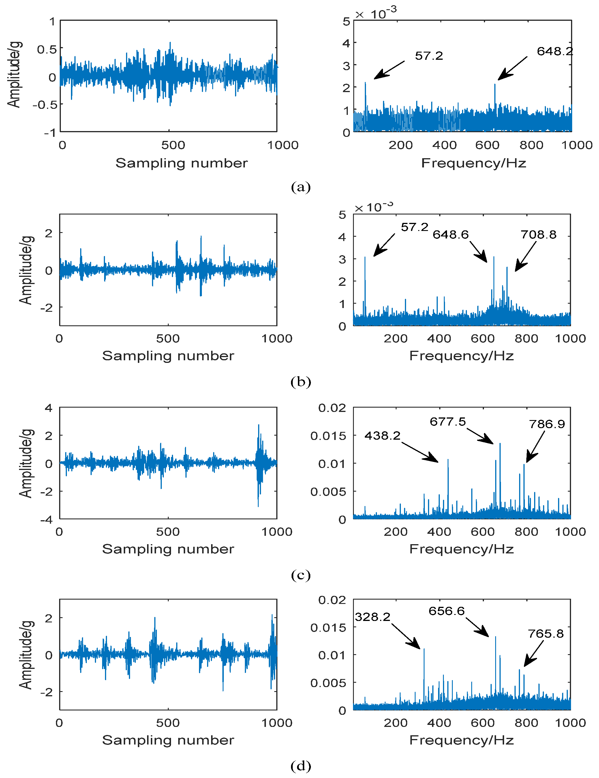
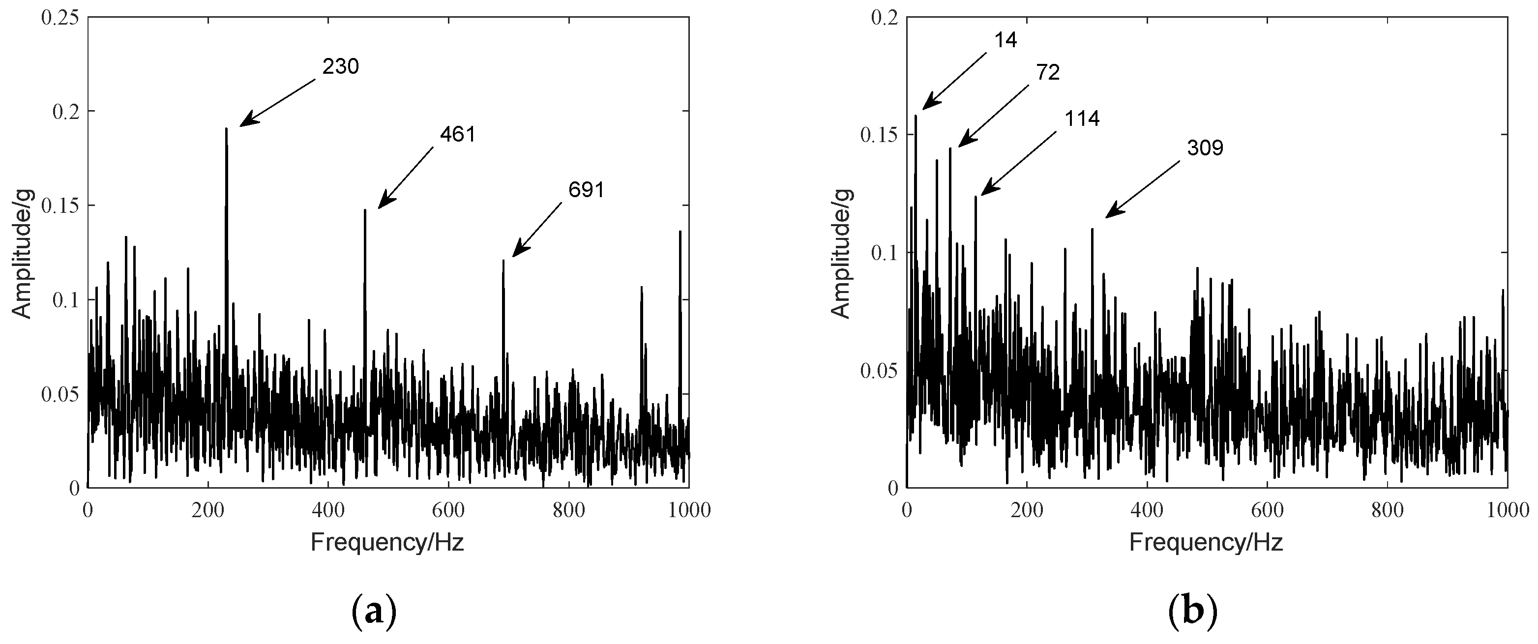
5. Envelope Spectrum Analysis

Empirical Mode Decomposition (EMD) is a time frequency method that can adaptively decompose signals according to their own signal characteristics [42]. It has been widely used in various disciplines and engineering fields. The Hilbert transform is capable of demodulating a fault-related signal from high frequencies [43]. The envelope spectrum analysis combined with EMD and Hilbert transform can effectively diagnose the characteristic frequency of faults.

In this paper, the results of the evaluation are verified by envelope spectrum analysis. Firstly, the IMF component of the intrinsic mode function of the data is extracted by the EMD algorithm, and the IMF component with the correlation of the original signal greater than 0.5 is selected by the correlation coefficient criterion [44]. The IMF component selected in this paper is greater than 0.5, which is IMF1. The Hilbert transform is performed on the component, and then the transformed signal is Fourier transformed to obtain an envelope spectrum [45].

The results of the proposed method are demodulated by envelope spectrum analysis, and the results are shown in Figure 13. Among them, Figure 14a shows the analysis result of the 533th sample, and Figure 14b shows the analysis result of the 532th sample. It can be seen that there is an obvious spectrum peak at the frequency with 230 Hz in Figure 14a, which is close to the BPFO with 236.4 Hz. Also, an obvious harmonic frequency characteristic exists. Moreover, the envelope spectrum of 532th sample depicted in Figure 14b shows no obvious spectrum peak at the frequency close to the BPFO (the samples before the 532th sample show the same results). The fundamental reason for the difference between the failure characteristic frequency and the theoretical characteristic frequency is the existence of skidding effect [46]. Therefore, the RBF neural network model concludes that the initial failure results are consistent with the verification results.

6. Conclusions

In this paper, a method for evaluating the degradation of rolling bearing performance based on WPEE and RBF neural network is proposed.

—

The WPEE is used to deal with the non-stationary and nonlinear characteristics of the vibration signal.

—

The RBF neural network has the advantages of fast convergence speed, good approximation performance, and simple structure, which improves the accuracy and real-time performance of bearing performance degradation evaluation.

—

The effects of three different radial basis functions on performance degradation evaluation results are compared, and the superiority of the RBF neural network based on the Gaussian basis function is highlighted.

—

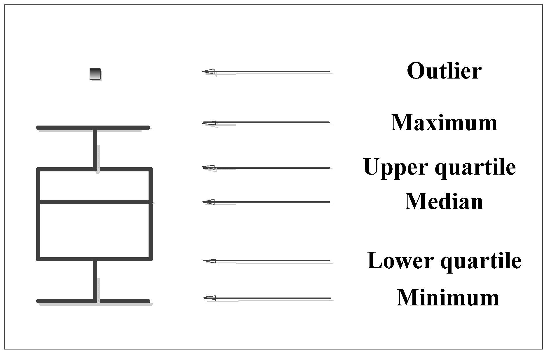
The box plot is used in the performance degradation assessment curve, and it is used as the alarm threshold method for bearing early fault determination. The box plot uses a quartile of certain robustness to calculate the actual appearance of the data. The results are objective and reliable, and can overcome the shortcomings of the previous failure thresholds that need to meet certain conditions.

In the experimental verification section, the feasibility of the model is verified by using different fault discrete data and full-life experimental data of rolling bearings. The results show that the method based on WPEE and the RBF neural network can distinguish between different degrees of bearing faults. Compared with the commonly used monitoring indicators, this method can find the early failure points of the bearing in a more quickly and timely way, and also provides a theoretical basis for the maintenance of the equipment. At the same time, it can effectively detect the performance degradation state of the bearing and reflect the degree of degradation of the rolling bearing’s operations.

References

- El-Thalji, I.; Jantunen, E. A summary of fault modelling and predictive health monitoring of rolling element bearings. Mech. Syst. Signal Process. 2015, 60, 252–272. [Google Scholar] [CrossRef]
- Zhou, Y. Research on Assessment Technology of Rolling Bearing Performance Degradation; University of Electronic Science and Technology of China: Chengdu, China, 2014. [Google Scholar]
- Wardle, F.P. Vibration Forces Produced by Waviness of the Rolling Surfaces of Thrust Loaded Ball Bearings Part 1: Theory. Proc. Inst. Mech. Eng. Part C J. Mech. Eng. Sci. 1988, 202, 305–312. [Google Scholar] [CrossRef]
- Takabi, J.; Khonsari, M. On the thermally-induced failure of rolling element bearings. Tribol. Int. 2016, 94, 661–674. [Google Scholar] [CrossRef]
- de Lacalle, L.N.L.; Lamikiz, A.; Sanchez, J.A.; de Bustos, I.F. Simultaneous Measurement of Forces and Machine Tool Position for Diagnostic of Machining Tests. IEEE Trans. Instrum. Meas. 2005, 54, 2329–2335. [Google Scholar]
- Lynagh, N.; Rahnejat, H.; Ebrahimi, M.; Aini, R. Bearing induced vibration in precision high speed routing spindles. Int. J. Mach. Tools Manuf. 2000, 40, 561–577. [Google Scholar] [CrossRef]
- Sopanen, J.; Mikkola, A. Dynamic model of a deep-groove ball bearing including localized and distributed defects. Part 1: Theory. Proc. Inst. Mech. Eng. Part K J. Multibody Dyn. 2003, 217, 201–211. [Google Scholar] [CrossRef]
- Chen, F.F.; Yang, Y.; Ma, J.H.; Chen, C. Fuzzy granulation prediction for bearing performance degradation based on information entropy and optimized LS-SVM. Chin. J. Sci. Instrum. 2016, 37, 779–787. [Google Scholar]
- Soualhi, A.; Medjaher, K.; Zerhouni, N. Bearing Health Monitoring Based on Hilbert–Huang Transform, Support Vector Machine, and Regression. IEEE Trans. Instrum. Meas. 2015, 64, 52–62. [Google Scholar] [CrossRef]
- Cheng, J.S.; Huang, W.Y.; Yang, Y. Feature Selection Method for Rolling Bearings’ Online Performance Degradation Assessment Based on LFSS and FSBBA. J. Vib. Shock 2018, 37, 89–94. [Google Scholar]
- Brkovic, A.; Gajic, D.; Gligorijevic, J.; Savic-Gajic, I.; Georgieva, O.; Di Gennaro, S. Early fault detection and diagnosis in bearings for more efficient operation of rotating machinery. Energy 2016, 136, 63–71. [Google Scholar] [CrossRef]
- Zhou, J.M.; Guo, H.J.; Zhang, L. Rolling Bearing Performance Degradation Assessment Based on Hidden Markov Model. J. East China Jiaotong Univ. 2017, 34, 110–116. [Google Scholar]
- Zhang, S.; Tang, J. Integrating angle-frequency domain synchronous averaging technique with feature extraction for gear fault diagnosis. Mech. Syst. Signal Process. 2018, 99, 711–729. [Google Scholar] [CrossRef]
- Yang, D.W.; Feng, F.Z.; Zhao, Y.A.; Jiang, P.C.; Ding, C. A VMD sample entropy feature extraction method and its application in planetary gearbox fault diagnosis. J. Vib. Shock 2018, 37, 198–205. [Google Scholar]
- Wan, S.T.; Zhang, X. Teager energy entropy ratio of wavelet packet transform and its application in bearing fault diagnosis. Entropy 2018, 20, 388. [Google Scholar] [CrossRef]
- Ma, J.; Wu, J.; Wang, X. Fault diagnosis method based on wavelet packet-energy entropy and fuzzy kernel extreme learning machine. Adv. Mech. Eng. 2018, 10, 1–14. [Google Scholar] [CrossRef]
- Li, S.L.; Liu, Z.L. Application of improved wavelet packet energy entropy and GA-SVM in rolling bearing fault diagnosis. In Proceedings of the 2018 IEEE International Conference on Signal Processing, Communications and Computing (ICSPCC), Qingdao, China, 14–16 September 2018. [Google Scholar]
- Liu, R.; Yang, B.; Zio, E.; Chen, X. Artificial intelligence for fault diagnosis of rotating machinery: A review. Mech. Syst. Signal Process. 2018, 108, 33–47. [Google Scholar] [CrossRef]
- Cong, H.; Xie, J.L.; Zhang, L.X.; Feng, F.Z. Evaluation of bearing performance degradation based on GA-SVDD. J. Armored Force Eng. Inst. 2012, 26, 26–30. [Google Scholar]
- Widodo, A.; Yang, B.S. Machine health prognostics using survival probability and support vector machine. Expert Syst. Appl. 2011, 38, 8430–8437. [Google Scholar] [CrossRef]
- Jianbo, Y. Bearing performance degradation assessment using locality preserving projections and Gaussian mixture models. Mech. Syst. Signal Process. 2011, 25, 2573–2588. [Google Scholar]
- Muruganatham, B.; Sanjith, M.; Krishnakumar, B.; Murty, S.S. Roller element bearing fault diagnosis using singular spectrum analysis. Mech. Syst. Signal Process. 2013, 35, 150–166. [Google Scholar] [CrossRef]
- Ben Ali, J.; Chebel-Morello, B.; Saidi, L.; Malinowski, S.; Fnaiech, F. Accurate bearing remaining useful life prediction based on Weibull distribution and artificial neural network. Mech. Syst. Signal Process. 2015, 56, 150–172. [Google Scholar] [CrossRef]
- Durodola, J.; Ramachandra, S.; Gerguri, S.; Fellows, N. Artificial neural network for random fatigue loading analysis including the effect of mean stress. Int. J. Fatigue 2018, 111, 321–332. [Google Scholar] [CrossRef] [Green Version]
- Al-Abdullah, A.L.; Abdi, H.; Lim, C.P.; Yassin, W.A. Force and temperature modelling of bone milling using artificial neural networks. Measurement 2018, 116, 25–37. [Google Scholar] [CrossRef]
- Hong, S.; Zhou, Z.; Zio, E.; Hong, K. Condition assessment for the performance degradation of bearing based on a combinatorial feature extraction method. Digit. Signal Process. 2014, 27, 159–166. [Google Scholar] [CrossRef]
- Lu, C.; Yuan, H.; Tang, Y. Bearing Performance Degradation Assessment and Prediction Based on EMD and PCA-SOM. J. Vibroeng. 2014, 16, 1387–1396. [Google Scholar]
- Liu, Y.Q.; Xu, Q.; Tian, D.; Long, Q. Bearing Performance Degradation Assessment Using Optimized BP Neural Network based on Glowworm Swarm Optimization Algorithm. J. Mech. Transm. 2014, 38, 107–109. [Google Scholar]
- Arnaiz-González, Á.; Fernández-Valdivielso, A.; Bustillo, A.; de Lacalle, L.N.L. Using artificial neural networks for the prediction of dimensional error on inclined surfaces manufactured by ball-end milling. Int. J. Adv. Manuf. Technol. 2016, 83, 847–859. [Google Scholar] [CrossRef]
- Dhimish, M.; Holmes, V.; Mehrdadi, B.; Dales, M. Comparing Mamdani Sugeno Fuzzy Logic and RBF ANN Network for PV Fault Detection. Renew. Energy 2018, 117, 257–274. [Google Scholar] [CrossRef]
- Zhao, N.B.; Yang, L.; Zheng, H.T.; Wang, Z. A Fault Diagnosis Approach for Rolling Element Bearing Based on S-transform and Artificial Neural Network. In Proceedings of the ASME Turbo Expo 2017: Turbomachinery Technical Conference and Exposition, Charlotte, NC, USA, 26–30 June 2017. [Google Scholar]
- Yu, B.; Xu, X.J.; Zheng, T. Application Research on Wavelet Packet-based Energy Feature Extraction for Fault Diagnosis of Rotating Machinery. Control Instrum. Chem. Ind. 2016, 43, 1056–1059. [Google Scholar]
- Lian, L.M.; Tang, J. Application of RBF Neural Network in Prediction of Static Stiffness for Constant-Current Hydrostatic Bearings. Bearing 2014, 2, 36–38. [Google Scholar]
- Guan, S.; Gao, J.W.; Zhang, B.; Liu, X.; Leng, Z.W. Traffic Flow Prediction Based on K-Means Clustering Algorithm and RBF Neural Network. J. Qingdao Univ. 2014, 29, 20–23. [Google Scholar]
- Hua, L.; Yu, H.C.; Shao, C.; Gong, S. Monitoring and Diagnosis of Abnormal Condition in Ethylene Production Process Based on SVM-BOXPLOT. CIESC J. 2017, 69, 1053–1063. [Google Scholar]
- Liu, Z.X.; Kang, J.S.; Qu, F.M.; Deng, Y.C. State Identification of Rolling Bearing Based on Noise Manifold Learning Algorithm. Fire Control Command Control 2018, 43, 127–130. [Google Scholar]
- Zhou, J.M.; Xu, Q.Y.; Zhang, L.; Li, H. Rolling Bearing Performance Degradation Assessment Based on the Wavelet Packet Tsallis Entropy and FCM. J. Mech. Transm. 2016, 40, 110–115. [Google Scholar]
- He, Z.J.; Chen, J.; Wang, T.Y.; Chu, F. Theories and Applications of Machinery Fault Diagnostics; Higher Education Press: Beijing, China, 2010. [Google Scholar]
- Hu, S.J.; Qian, Y.N.; Yan, R.Q. Anomaly Detection Using Symbolic Time Series Analysis Based on Probability Density Space Partitioning. J. Vib. Eng. 2014, 27, 780–784. [Google Scholar]
- Zhu, S.; Bai, R.L.; Liu, Q.H. Rolling Bearing Performance Degradation Assessment Based on FOA-WSVDD. China Mech. Eng. 2018, 29, 602–608. [Google Scholar]
- Wang, H.; Ji, Y.; Zhu, L.B.; Liu, X. Performance degradation evaluation of mechanical equipment based on HOP-CHMM. J. Vib. Meas. Diagn. 2018, 38, 91–95. [Google Scholar]
- Wu, Z.T.; Yang, S.X. A New Method for Fault Feature Extraction and Pattern Classification of Rotating Machinery; Science Press: Beijing, China, 2012. [Google Scholar]
- Su, W.S.; Wang, F.T.; Zhang, Z.X.; Guo, Z.G. Application of EMD Denoising and Spectral Kurtosis in Early Fault Diagnosis of Rolling Element Bearings. J. Vib. Shock 2010, 29, 18–21. [Google Scholar]
- Jiang, Q.; Li, T.; Yao, Y.; Cai, J. Study of Rolling Bearing SVM Pattern Recognition Based on Correlation Dimension of IMF. In Proceedings of the Second International Conference on Intelligent System Design and Engineering Application, Sanya, Hainan, China, 6–7 January 2012; pp. 1132–1135. [Google Scholar]
- Zhou, J.M.; Guo, H.J.; Zhang, L.; Xu, Q.; Li, H. Bearing Performance Degradation Assessment Using Lifting Wavelet Packet Symbolic Entropy and SVDD. Shock Vib. 2016, 2016, 1–10. [Google Scholar] [CrossRef] [Green Version]
- Niu, L.; Cao, H.; He, Z.; Li, Y. A systematic study of ball passing frequencies based on dynamic modeling of rolling ball bearings with localized surface defects. J. Sound Vib. 2015, 357, 207–232. [Google Scholar] [CrossRef]