Image Enhancement Using Modified Histogram and Log-Exp Transformation

Abstract

An effective method to enhance the contrast of digital images is proposed in this paper. A histogram function is developed to make the histogram curve smoother, which can be used to avoid the loss of information in the processed image. Besides the histogram function, an adaptive gamma correction for the histogram is proposed to stretch the brightness contrast. Moreover, the log-exp transformation strategy is presented to progressively increase the low intensity while suppressing the decrement of the high intensity. In order to further widen the dynamic range of the image, the nonlinear normalization transformation is put forward to make the output image more natural and clearer. In the experiment on non-uniform illumination images, the average contrast per pixel (CPP), root mean square (RMS), and discrete entropy (DE) metrics of the developed approach are shown to be superior to selected state-of-the-art methods.

1. Introduction

Enhancement technology is regarded as one of the most fundamental problems in computer vision. It can be widely used in many applications such as monitoring, imaging systems, human–computer interactions, and so on [1,2,3]. In many cases, the contrast in digital video or images is poor, which can be caused by many circumstances including a lack of operator expertise and inadequacy of the image acquisition equipment. In most cases, the captured scenes are under unfavorable environmental conditions—for example, the presence of clouds, the lack of sunlight, backlight or indoor lighting, and so on. These conditions might also result in reduced contrast quality. In view of the above problems, many researchers still concentrate on poor contrast image enhancement [4,5]. Generally speaking, the enhancement techniques for poor contrast images are broadly made up of two categories: direct enhancements [6,7,8] and indirect enhancements [9,10,11]. The direct enhancement methods [6,7,8] can directly define the image contrast by a specific contrast term. Most of these metrics, however, cannot simultaneously measure the contrast of simple and complex patterns in images. Various image enhancement techniques have been presented [12,13,14,15,16] to enhance the contrast of an image. For instance, histogram equalization (HE) is a widely used technique that is simple and easily implemented [13]. Unfortunately, HE [13] does not always give satisfactory results since it might cause annoying artifacts and intensity saturation effects [16].

Scholars have proposed many other HE-based methods, such as brightness preserving bi-histogram equalization (BBHE) [15], dualistic sub-image histogram equalization (DSIHE) [17], and minimum mean brightness error bi-histogram equalization (MMBEBHE) [18]. BBHE [15] divides the histogram based on the image, meanwhile DSIHE [17] uses the image median to partition the histogram. The method of six threshold plateau limits for a segmented histogram [19] was introduced to improve the BBHE method by Lim et al. The image histogram is recursively segmented into multiple groups based on the mean brightness error (MBE) in MMBEBHE [18] method. The methods mentioned above have enabled great progress in the field. However, there are some drawbacks including failure in images with non-symmetric distribution [15], the loss of structural information [16], the preservation of the mean brightness [17], and the production of annoying side effects [18]. Therefore, these algorithms have failed to achieve the desired improvements in contrast enhancement. Moreover, the difference between the input and output image can be minimal when using these methods [20].

To overcome the limitations mentioned above, recursive mean-separate histogram equalization (RMSHE) [21] was proposed for the recursive division of histograms based on the local mean. The average brightness of the processed image is close to that of the input image. Adaptively modified histogram equalization (AMHE) [22] was proposed to modify the probability density function (PDF) of the grayscale. AMHE [22] does not produce any degradation. However, it darkens the bright areas and fails to boost the brightness of the dark regions. Recursive sub-image histogram equalization (RSIHE) [23] based on contrast enhancement was developed to improve DSIHE [17], and the recursive segmentation was introduced in a similar manner to that reported in [21]. Hasikin et al. [24] proposed an adaptive fuzzy intensity measurement method that can selectively enhance the dark area of the image without brightening the bright area.

Some other methods based on histogram equalization have been introduced, which can enhance the contrast of images with brightness. Dynamic histogram specification [25] was developed to preserve the shape of the input image histogram without significant enhancement. A contrast enhancement algorithm was developed in [26,27] for color images. Adaptive gamma correction with weighting distribution (AGCWD) [28] was presented to enhance brightness and preserve the available histogram information. Although AGCWD [28] enhances the contrast and preserves the overall brightness of an image, it may not give the desired results. If the maximum intensity of the output image is limited by the maximum intensity of the input image, the input image will lack bright pixels [29]. An image enhancement technique called exposure sub-image histogram equalization (ESIHE) [30] was developed. This technique divides the clipped histogram into two parts according to the pre-calculated exposure threshold [31]. The intensity exposure in histogram segmentation before histogram clipping was developed to enhance the image [32]. This shows that the threshold value computed from the intensity exposure of the image is employed to divide the input histogram, which can yield certain enhancement results. However, it usually causes under-enhancement. Bi-histogram equalization in modified histogram bins (BHEMHB) [33] was developed to segment the input histogram based on the median brightness of an image, which alters the histogram bins before HE [13]. Unfortunately, it makes limited improvement in the contrast.

A novel image enhancement method is proposed through adaptive gamma correction with reasonable histogram function in this paper. This method can improve the low intensity of the image and avoid the significant decrement of the high intensity; thus, the dynamic range of the image is effectively extended. The main contributions of this paper are as follows: Firstly, a novel histogram function is developed to modify the histogram of the image, which can be used to make the resultant transformation curve smoother. This can avoid the loss of some information in the processed image. Secondly, log-exp transformation (LET) is proposed to make the weighted values in the dark regions of the image higher while the ones in the bright regions are lower. In addition, a nonlinear normalization transformation (NNT) is put forward to obtain a wider dynamic range for the brightness component of the output image. This makes the output image more natural and clearer. The third important contribution is that the image can be enhanced using ordinary hardware without the need to hypothesize the scenario contents in advance. The extensive experimental comparisons with state-of-the-art methods show the superior performance of the proposed method.

An overall flowchart for image enhancement is shown in Figure 1.

The rest of the paper is organized as follows. The modified histogram-based enhancement is described in Section 2. The experimental results and analyses are discussed in Section 3. Some conclusions follow in Section 4.

2. Modified Histogram-Based Enhancement

The HSV (Hue, Saturation, Value) color space is selected to deal with the color image processing, since it has some advantages such as a color representation for human perception and color information separation from the brightness (or lightness) information [34]. In the HSV color space, the color contents are represented by H (hue) and S (saturation), whereas the luminance intensity is represented by V(luminance value). To eliminate the side effects of false color, the proposed method only enhances the V component, while the H and S components remain unchanged.

2.1. Adaptive Gamma Correction with Modified Histogram

Gamma correction methods constitute a series of general histogram modifications techniques that can be obtained simply by using the variable adaptive parameter γ. The simple form of gamma correction based on the transformation is described as:

$$T(l)=l_{\max }{(l/l_{\max })}^{\gamma }$$

(1)

where l_max denotes the maximum intensity of the input image. After executing Formula (1), the intensity l of each pixel in the input image is converted to T(l). However, when the contrast is directly modified by gamma correction, the different images exhibit the same intensity changes due to the fixed parameters. Fortunately, this problem can be solved by calculating the probability density of each intensity level in the digital image.

The AGCWD [28] algorithm modifies the statistical histogram and lessens the generation of adverse effects by applying the weighting distribution (WD) function. The WD function is defined as:

$$pd{f}_w(l)=pd{f}_{\max }{\left(\frac{pdf(l)-pd{f}_{\min }}{pd{f}_{\max }-pd{f}_{\min }}\right)}^{\alpha }$$

(2)

where pdf_max is the maximum of probability density function, pdf_min is the minimum, and α is an adjusted parameter, which is set at 0.8 in [28].

The cdf_w(l)is approximated as:

$$cd{f}_w(l)={\displaystyle \sum _{k=0}^{l_{}}pd{f}_w(k)/{\displaystyle \sum pd{f}_w}}$$

(3)

where cdf denotes the cumulative distribution function, and the sum of pdf_w is calculated as:

$${\displaystyle \sum pd{f}_w={\displaystyle \sum _{l=0}^{l_{\max }}pd{f}_w(l)}}$$

(4)

The resultant cdf curves of AGCWD [28] in α = 0.8 for front lighting #1 and the side lighting are shown in Figure 2. It can be seen that the resultant transformation curves do not increase smoothly for AGCWD [28] in α = 0.8.

To prove this viewpoint (in front lighting #1 α = 0.8) further, we can mark two intervals on the x-axis ((l₁, l₂), (l₃, l₄)) and their corresponding intervals on the y-axis ((c₁, c₂), (c₃, c₄), respectively). The small interval (l₁, l₂) is transformed to the sufficiently large interval (c₁, c₂). Some sufficient weights are correspondingly assigned to (3) in this case. When a large interval (l₃, l₄) is transformed to the small interval (c₃, c₄), the weight should be assigned to be a smaller one. This may lead to the loss of information in the processed image.

A modified histogram function is proposed to solve this problem as follows:

$$pd{f}_{wm}(l)=std{(L)}^{\sqrt{\frac{std(L)}{mean(L)}}}\times pd{f}_w{(l)}^{\delta }+(mean(L)+255)\times pd{f}_w(l)$$

(5)

where std(L) represents the variance value of the image luminance component, mean(L) is the mean value of the image luminance component, and δ is an adjusted parameter (this is discussed later).

The modified cdf_wm is calculated by:

$$cd{f}_{wm}(l)={\displaystyle \sum _{l=0}^{l_{\max }}pd{f}_{wm}(l)/{\displaystyle \sum pd{f}_{wm}}}$$

(6)

Figure 3 shows the cumulative distribution function curves in AGCWD [28] and the proposed method for δ = 0.5, respectively.

In Figure 3, it can be observed that the proposed method can avoid under-enhancement and over-enhancement in the low-intensity region of by smoothing the fluctuated parts. On the other hand, the high-intensity level is only slightly decreased to enhance the contrast with intensity preservation.

Adaptive gamma correction with modified histogram (AGCMH) is given correspondingly as:

$$L_{AGC}=T(l)=l_{\max }{\left(\frac{l}{l_{\max }}\right)}^{\gamma }$$

(7)

where $\gamma =1-cd{f}_{wm}(l)$.

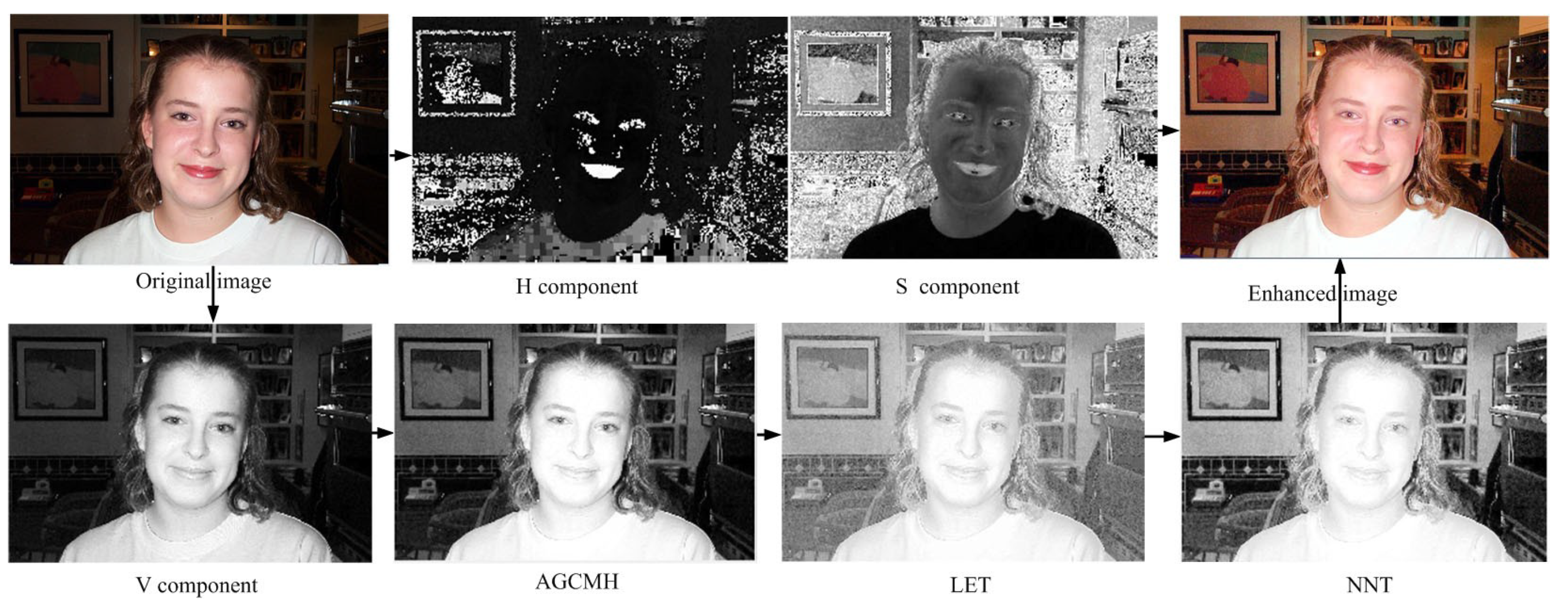
2.2. Log-Exp Transformation

Although the brightness contrast is stretched, it looks dark for some regions in the processed image as shown in Figure 1. The dark region should be processed further. A log-exp transformation (LET) was developed to cope with the illumination compensation of the image and preserve its naturalness, in which there is higher weight for the dark region and lower weight for the bright region. The LET is defined as follows:

$$T_{LET}=x^{({\log }_b^{}(L_{AGC}+a)+c)}$$

(8)

where $T_{LET}:{\Re }^{N\times N}\to {\Re }^{N\times N}$, $x=\max {(L_{AGC})}^{\left(1/\max ({\log }_b^{}(L_{AGC}+a)+c)\right)}$, the function max(•) calculates the maximum value of the matrix, a = mean(L_AGC), b = std(L_AGC), and c = mean(L_AGC)/std(L_AGC). The element of intensity matrix L_AGC is denoted as l_ij.

It can be found that T_LET is an increasing function from (8). A small value of l_ij would be sufficiently transformed to T_LET (l_ij) with a larger increment, while a large value of l_ij would be transformed to T_LET (l_ij) with a smaller increment after implementing (8). When l_ij reaches the maximum of L_AGC, the value of T_LET (l_ij) is equal to l_ij, as shown in Figure 4.

The transformation would cause the image to blur to a certain degree, as shown in Figure 1. A nonlinear normalization is proposed to deal with this effect in the next section.

2.3. Nonlinear Normalization Transformation

Nonlinear normalization transformation (NNT) was developed to deal with the blur problem exhibited by LET as follows:

$$L_{NNT}=T_{NNT}(l_{ij})=\chi \times l_{ij}^{-\mu }+\lambda$$

(9)

where μ is a variable parameter—when it is set to −1, (9) would be a linear normalization function. χ and λ are parameters to adjust the intensity of L_NNT within [0, 255] as follows:

$$\{\begin{array}{c}{T}_{NNT}(l_{\max })\times \chi +\lambda =255\\ T_{NNT}(l_{\min })\times \chi +\lambda =0\end{array}$$

(10)

After the nonlinear normalization transformation, the luminance range is within [0, 255].

To highlight the result, an example is given in Figure 5 for AGCMH, LET, and NNT. It can be seen that AGCMH causes the image histogram to appear sketched with some dark regions (Figure 5b). The dark region is brightened with blur to a certain extent after LET, as shown in Figure 5c. The dynamic range of the image is widened and the output image looks like natural and clear after NNT (Figure 5d).

3. Experimental Results and Analyses

To test the performance of the proposed approach, state-of-the-art methods were selected including RMSHE [21], AMHE [22], RSIHE [23], AGCWD [28], ESIHE [30], and BHEMHB [33]. The comparison was performed addressing both subjective and objective evaluations.

3.1. Parameter Analysis

To build a fair comparison, some parameters including δ in (4) and μ in (8) were set to constant values so that they were less influenced by the different scene contents. To determine reasonable values of δ and μ, 2000 images from [35,36,37,38] were selected to test the enhancement performance in average values of contrast per pixel (CPP) [39], root mean square (RMS) [40], and discrete entropy (DE) [41]. Figure 6 shows the statistical results for different values of δ and μ. It can be seen from Figure 6 that there were excellent performances when δ was 0.5 and μ was 0.7. Therefore, δ and μ were set to 0.5 and 0.7, respectively, and maintained at these values in the experiment.

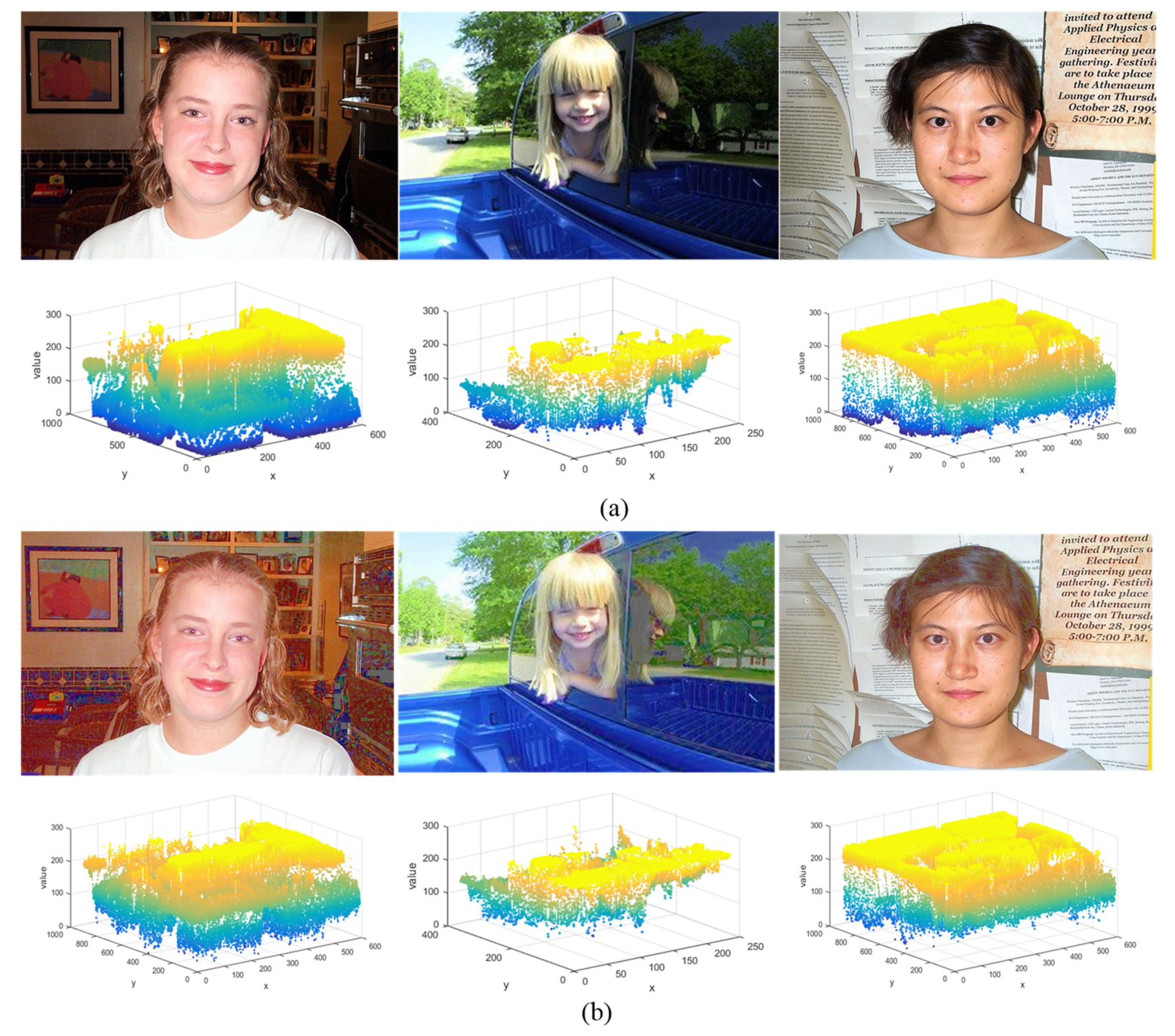
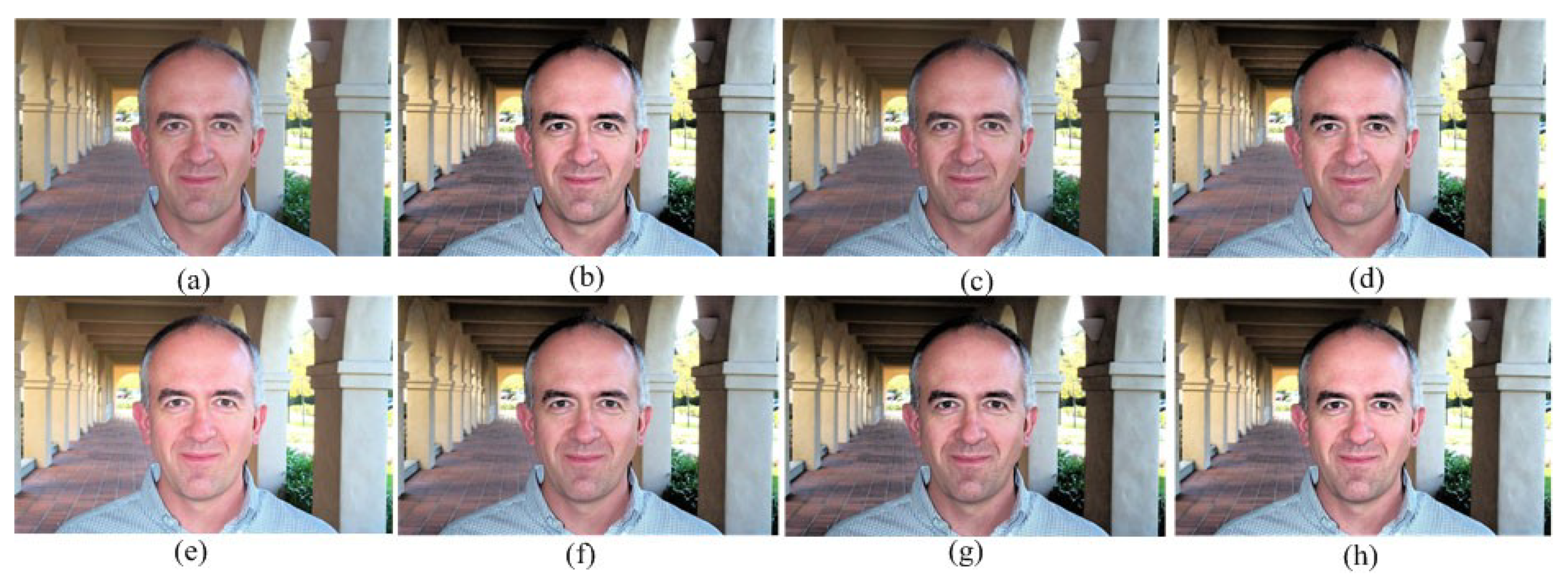
3.2. Subjective Evaluation

For the subjective evaluation, the test images were selected from DIP3/e Book Images [35], the Caltech faces 1999 dataset [36], NASA release images [37], and the Extended Yale B database [38]. The chosen images were classified as dim, backlighting, front lighting, daytime, side lighting, or gray. There were non-uniform illuminations for most of the selected images.

Some results are given in Figure 7 with the investigated methods for dim #1. Both RMSHE [21] and RSIHE [23] made improvements in the dark area with some gray-level loss in the bright area, as shown in Figure 7b,d, respectively. AMHE [22] equalized the original histogram without changes in the overall luminance, as shown in Figure 7c. Both AGCWD [28] and ESIHE [30] obtained a superior dynamic contrast as compared to the abovementioned methods. There were some dark regions, as shown in Figure 7e,f, respectively. The result of BHEMHB [33] was more natural than those of AGCWD [28] and ESIHE [30]. There were some unnatural regions, as shown in Figure 7g. However, it can be seen that the proposed method exhibited an excellent performance (Figure 7h).

Another example for dim #2 is given in Figure 8. RMSHE [21], AMHE [22], and RSIHE [23] improved the dark region with the low level of brightness, providing a weak enhancement, as shown in Figure 8b–d, respectively. An outstanding result of AGCWD [28] was demonstrated, apart from some regions with dark brightness. ESIHE [30] and BHEMHB [33] enhanced the contrast of the image and preserved its original features. However, it looked somewhat unnatural, as shown in Figure 8f,g, respectively. It can be noted that a clearer result was achieved by the proposed method, as shown in Figure 8h.

Some enhancement results for a backlighting image using different methods are shown in Figure 9.

There are poor illuminations due to the backlighting in the image shown in Figure 9a. RMSHE [21], AMHE [22], and RSIHE [23] achieved improvements in the facial region. There were some dark and unnatural regions, especially in the facial areas, as shown in Figure 9b–d, respectively. Some information was lost in AGCWD [28] due to the unreasonable cdf curve, as shown in Figure 9e. Both ESIHE [30] and BHEMHB [33] enhanced the contrast and preserved the color information to some extent. It still looked somewhat dark, as shown in Figure 9f,g, respectively. Meanwhile, the proposed method achieved a more natural and clearer result (Figure 9h).

Some enhancement results for front lighting #1 using different methods are shown in Figure 10. Both RMSHE [21] and RSIHE [23] led to improvements in the background. Some gray-level information was lost in the facial region, as shown in Figure 10b,d, respectively. AMHE [22] compressed the dynamic range of the image and resulted in a blurred image, as shown in Figure 10c. AGCWD [28] also achieved improvement in the background. There was an oversaturated area in the facial region, as shown in Figure 10e. Both ESIHE [30] and BHEMHB [33] obtained a superior dynamic range. There were some dark regions, as shown in Figure 10f,g. However, excellent visual quality for human beings was achieved in the proposed method, as shown in Figure 10h.

Some enhancement results for front lighting #2 with different methods are shown in Figure 11. RMSHE [21], AMHE [22] and RSIHE [23] showed improvements in the contrast sketch, as shown in Figure 11b–d, respectively. AGCWD [28] achieved a fine dynamic range. There were some dark regions still apparent in Figure 11e. Both ESIHE [30] and BHEMHB [33] showed high visibility. There were some over-enhancements in the facial regions, as shown in Figure 11f,g. The proposed method gave a more natural and clearer image, as shown in Figure 11h.

Some enhancements for both daytime #1 and #2 using different methods are shown in Figure 12 and Figure 13, respectively. It can be seen that a superior enhancement performance was given by the proposed method as compared to the other methods in Figure 12 and Figure 13.

Some enhancements for side lighting are shown in Figure 14. RMSHE [21], AMHE [22], and RSIHE [23] gave improvements in the shadow areas with inconsistent luminance. However, there were still some dark regions, as shown in Figure 14b–d. AGCWD [28] achieved a fine dynamic brightness range. Yet, the image looked both unnatural and unclear for human vision, as shown in Figure 14e. Both ESIHE [30] and BHEMHB [33] improved the visibility and enhanced the details, and the dynamic range was compressed, as shown in Figure 14f,g, respectively. Meanwhile, the transition between brightness and darkness was smooth in the image following the proposed method. Moreover, the processed image texture became clearer, as shown in Figure 14g.

Another enhancement example for a gray image is shown in Figure 15. RMSHE [21] led to over-enhancement in the bright region, as shown in Figure 15b. Both AMHE [22] and RSIHE [23] obtained limited improvements in the dark region, as shown in Figure 15c,d, respectively. AGCWD [28] improved the visibility to some extent. The image was a little blurred since this method compressed the dynamic range of brightness, as shown in Figure 15e. Both ESIHE [30] and BHEMHB [33] caused some details to stand out. However, the image still looked dark due to its limited improvement in brightness. The proposed method had the best visibility and naturalness, as shown in Figure 15h.

3.3. Objective Evaluations

To further test the enhancement performance quantitatively, CPP [39], RMS [40], and DE [41] were employed to perform a comparison of the proposed method with some of the state-the-art approaches mentioned above.

3.3.1. Contrast Per Pixel (CPP)

CPP [39] indicates the degree of variation in the surrounding pixels. Its characteristics are proportional to the contrast. It can measure the degree of detailed expression of an M × N images follows:

$$CPP=\frac{{\displaystyle {\sum }_{i=o}^{M-1}{\displaystyle {\sum }_{j=0}^{N-1}(\frac{1}{9}{\displaystyle {\sum }_{m=-1}^1{\displaystyle {\sum }_{n=-1}^1|\overline{l_{(i,j)}}-}}\overline{l_{(i+m,j+n)}}|)}}}{MN}$$

(11)

where l indicates the luminance element of the image.

Some results are given in

Table 1. Objective evaluation results in term of CPP.

Image	RMSHE [21]	AMHE [22]	RSIHE [23]	AGCWD [28]	ESIHE [30]	BHEMHB [33]
Dim #1	6.92	3.32	7.55	5.33	4.16	5.11
Dim #2	11.06	6.64	9.66	10.92	9.42	7.27
Backlighting	16.85	15.77	16.84	17.13	15.72	15.21
Front Lighting #1	6.17	4.50	5.60	4.95	5.01	6.15
Front Lighting #2	5.87	5.98	7.16	7.69	7.05	7.45
Daytime #1	9.41	8.08	9.30	7.45	8.95	9.56
Daytime #2	13.13	12.38	13.36	11.33	12.35	12.67
Side Lighting	9.60	10.13	9.30	11.57	9.49	9.66
Gray	9.30	8.38	9.24	7.36	8.13	9.60
Average	9.81	8.35	9.81	9.30	8.92	9.19

for CPP [39] obtained by the investigated methods mentioned above.

It can be seen from Table 1 that the proposed method outperforms the comparison algorithms in CPP [39] as a whole.

To further highlight the performance of the proposed method, 2000 images were divided into five groups. Each group contained 400 images. The groups included backlight (G1), daytime (G2), front lighting (G3), dim (G4), and side lighting (G5) images. We computed their corresponding CPP values, as given in

Table 2. CPP performance in five groups comparisons with different methods.

Image	G1	G2	G3	G4	G5	Average
RMSHE [21]	8.68	9.20	7.35	4.79	5.45	7.09
AMHE [22]	7.99	7.35	6.48	3.57	4.37	5.95
RSIHE [23]	8.58	8.09	6.96	5.58	5.00	6.84
AGCWD [28]	8.20	7.85	8.04	4.62	5.17	6.78
ESIHE [30]	8.59	8.73	7.62	4.28	4.44	6.73
BHEMHB [33]	8.79	8.77	7.89	4.66	5.13	7.05
Proposed	8.84	8.58	8.48	7.68	6.03	7.92

.

It can be further found from Table 2 that among the methods investigated for comparison, the best enhancement performance was achieved by the developed method.

3.3.2. Root Mean Square (RMS)

RMS is a common way to measure the contrast of an image [40], where a higher value indicates the better visibility of the output image. The RMS [40] is defined as:

$$RMS=\sqrt{\frac{1}{MN}{{\displaystyle {\sum }_{i=o}^{M-1}{\displaystyle {\sum }_{j=0}^{N-1}(\mu -l_{(i,j)})}}}^2}$$

(12)

where μ represents the mean of the input image, l indicates the luminance element of the input image, and M and N represent the width and height of the image, respectively.

Some results for the RMS are given in

Table 3. Objective evaluation results in term of RMS.

Image	RMSHE [21]	AMHE [22]	RSIHE [23]	AGCWD [28]	ESIHE [30]	BHEMHB [33]	Proposed
Dim #1	72.41	45.30	72.95	77.78	62.98	43.57	79.12
Dim #2	72.38	38.55	63.32	64.84	54.41	38.48	72.22
Backlighting	82.58	78.46	81.48	82.18	81.29	77.51	84.45
Front Lighting #1	74.33	72.05	76.37	88.05	75.44	73.65	83.59
Front Lighting #2	69.07	79.08	82.26	87.49	76.70	68.40	87.91
Daytime #1	74.13	58.19	67.12	58.55	65.27	71.15	75.70
Daytime #2	71.23	60.88	64.10	63.40	61.38	60.82	72.11
Side Lighting	73.94	73.33	72.30	82.01	71.51	64.7	77.86
Gray	67.71	58.55	66.08	54.95	56.76	62.08	70.47
Average	73.09	62.71	71.78	73.25	67.30	62.26	78.16

and

Table 4. RMS performance in five groups comparisons with different methods.

Method	G1	G2	G3	G4	G5	Average
RMSHE [21]	77.57	71.75	73.23	58.47	69.32	70.07
AMHE [22]	80.47	62.97	65.71	39.82	67.73	63.34
RSIHE [23]	83.92	66.51	68.14	63.25	71.72	70.71
AGCWD [28]	83.44	66.84	75.08	58.74	88.16	74.45
ESIHE [30]	73.97	69.27	68.85	68.67	68.57	69.87
BHEMHB [33]	73.89	31.34	68.85	40.91	57.67	54.53
Proposed	84.24	72.45	75.18	73.90	83.95	77.94

[40] with the investigated methods mentioned above. As indicated in Table 3, the RMSHE method obtained the best result for the dim #2 image, and AGCWD reached the highest RMS value for the front lighting #1 and side lighting images. The proposed algorithm performed best in all other images. The proposed method acquired the highest value in all groups except G5, and the highest average value was also obtained by our algorithm.

The best enhancement performances by the developed method is shown among the other investigated methods, as shown in Table 3 and Table 4.

3.3.3. Discrete Entropy (DE)

According to the information theory, the richness of information in the image can be determined by Shannon entropy. The greater the entropy value of the image, the higher the information contained in the output image will have [41]. The discrete entropy (DE) for the whole image of the gray-level l can be defined as:

$$DE=-{\displaystyle \sum _{l=0}^{L-1}p(l){\log }_{2}p(l)}$$

(13)

Only if p(0) = p(1) = ... = p(L − 1) = 1/L can the entropy of the image achieve its maximum. This is the case when the probability distribution of image intensity values is uniform. Some results are given in

Table 5. Objective evaluation results in term of DE.

Image	RMSHE [21]	AMHE [22]	RSIHE [23]	AGCWD [28]	ESIHE [30]	BHEMHB [33]	Proposed
Dim #1	6.83	6.75	7.19	7.35	7.14	7.25	7.91
Dim #2	7.20	7.02	6.98	7.53	7.38	7.14	7.90
Backlighting	7.35	7.29	7.34	7.30	7.22	7.26	7.38
Front Lighting #1	7.98	7.74	7.89	7.60	7.86	7.96	7.79
Front Lighting #2	7.60	7.69	7.66	7.50	7.84	7.83	7.86
Daytime #1	7.80	7.62	7.77	7.34	7.75	7.67	7.87
Daytime #2	7.67	7.71	7.65	7.10	7.64	7.67	7.69
Side Lighting	7.62	7.69	7.60	7.67	7.68	7.71	7.75
Gray	7.35	7.45	7.35	6.47	7.25	7.56	7.61
Average	7.49	7.44	7.49	7.32	7.53	7.56	7.75

and

Table 6. DE performance in five groups comparisons with different methods.

Method	G1	G2	G3	G4	G5	Average
RMSHE [21]	7.47	7.87	7.65	5.87	7.36	7.24
AMHE [22]	7.47	7.72	7.73	6.52	7.07	7.3
RSIHE [23]	7.52	7.75	7.67	5.83	6.97	7.15
AGCWD [28]	7.22	7.39	7.63	6.59	7.06	7.18
ESIHE [30]	7.51	7.85	7.61	6.51	6.87	7.27
BHEMHB [33]	7.53	7.84	7.76	6.75	7.2	7.42
Proposed	7.68	7.66	7.76	7.24	7.37	7.54

for the values of DE achieved using the investigated methods mentioned above.

It can be further found from Table 5 and Table 6 that there are the best enhancement performances are exhibited by the developed method as compared to the other investigated approaches.

We note that the proposed method can be applied to effectively improve the visibility, contrast, and brightness of non-uniform illumination, as well as preserve image details. This method was shown to mathc or exceed the performances of other selected state-of-the-art methods.

In order to test its performance in real-time processing, we used images with the size of 896 × 592 pixels for further testing. All the experiments were run in MATLAB 2016 on a PC with 3.3 GHz CPU and 4 GB RAM.

Table 7. Average running time (s).

RMSHE [21]	AMHE [22]	RSIHE [23]	AGCWD [28]	ESIHE [30]	BHEMHB [33]	Proposed
0.21	0.26	0.23	0.30	0.18	0.19	0.17

shows the average running time of different methods. The proposed method obtained a superior performance in real-time processing compared with most of the other algorithms.

4. Conclusions

In this paper, an effective method to enhance the contrast of digital images was presented. The histogram of the input image was modified by a novel function, which can avoid the loss of information in the image processing procedure. The log-exp transformation was developed to make the weighted values in the dark regions of the image higher while the ones in the bright regions were lower. In order to obtain a wider dynamic range for the brightness component of the output image, a nonlinear normalization transformation was put forward. The clearness of non-uniform illumination images was obviously improved following the application of the proposed method. The experimental results show that the proposed method has a better image enhancement performance compared with other state-of-the-art methods.

References

1. Du, S.; Ward, R.K. Adaptive region-based image enhancement method for robust face recognition under variable illumination conditions. IEEE Trans. Circuits Syst. Video Technol. 2010, 20, 1165–1175. [Google Scholar] [CrossRef]
2. Sun, G.; Liu, S.; Wang, W.; Chen, Z. Dynamic range compression and detail enhancement algorithm for infrared image. Appl. Opt. 2014, 53, 6013–6029. [Google Scholar] [CrossRef] [PubMed]
3. Huang, T.; Shih, K.; Yeh, S.; Chen, H. Enhancement of backlight-scaled images. IEEE Trans. Image Process. 2013, 22, 4587–4597. [Google Scholar] [CrossRef] [PubMed]
4. Atta, R.; Ghanbari, M. Low-contrast satellite images enhancement using discrete cosine transform pyramid and singular value decomposition. IET Image Process. 2013, 7, 472–483. [Google Scholar] [CrossRef]
5. Han, H.; Sohn, K. Automatic illumination and color compensation using mean shift and sigma filter. IEEE Trans. Consum. Electr. 2009, 55, 978–986. [Google Scholar] [CrossRef]
6. Beghdadi, A.; Le Negrate, A. Contrast enhancement technique based on local detection of edges. Comput. Vis. Image Und. 1989, 46, 162–174. [Google Scholar]
7. Cheng, H.D.; Xu, H. A novel fuzzy logic approach to contrast enhancement. Pattern Recognit. 1989, 33, 809–819. [Google Scholar] [CrossRef]
8. Tang, J.; Liu, X.; Sun, Q. A direct image contrast enhancement algorithm in the wavelet domain for screening mammograms. IEEE J. Sel. Top. Signal Process. 2009, 3, 74–80. [Google Scholar] [CrossRef]
9. Sherrier, R.H.; Johnson, G.A. Regionally adaptive histogram equalization of the chest. IEEE Trans. Med. Imaging 1987, 6, 1–7. [Google Scholar] [CrossRef]
10. Polesel, A.; Ramponi, G.; Mathews, V.J. Image enhancement via adaptive unsharp masking. IEEE Trans. Image Process. 2000, 9, 505–510. [Google Scholar] [CrossRef] [Green Version]
11. Chiu, Y.S.; Cheng, F.C.; Huang, S.C. Efficient contrast enhancement using adaptive gamma correction and cumulative intensity distribution. In Proceedings of the IEEE International Conference on Systems, Man, and Cybernetics, Anchorage, AK, USA, 9–12 October 2011; pp. 2946–2950. [Google Scholar]
12. Cheng, H.D.; Shi, X.J. A simple and effective histogram equalization approach to image enhancement. Digit Signal Process. 2004, 14, 158–170. [Google Scholar] [CrossRef]
13. Coltuc, D.; Bolon, P.; Chassery, J.M. Exact histogram specification. IEEE Trans. Image Process. 2006, 15, 1143–1152. [Google Scholar] [CrossRef] [PubMed]
14. Hussain, K.; Rahman, S.; Khaled, S.M.; Abdullah-Al-Wadud, M.; Shoyaib, M. Dark image enhancement by locally transformed histogram. In Proceedings of the IEEE International Conference on Software, Knowledge, Information Management and Applications, Dhaka, Bangladesh, 18–20 December 2014; pp. 1–7. [Google Scholar]
15. Kim, Y.T. Contrast enhancement using brightness preserving bihistogram equalization. IEEE Trans. Consum. Electr. 1997, 43, 1–8. [Google Scholar]
16. Kim, M.; Chung, M.G. Recursively separated and weighted histogram equalization for brightness preservation and contrast enhancement. IEEE Trans. Consum. Electr. 2008, 54, 1389–1397. [Google Scholar] [CrossRef]
17. Wang, Y.; Chen, Q.; Zhang, B. Image enhancement based on equal area dualistic sub-image histogram equalization method. IEEE Trans. Consum. Elect. 1999, 45, 68–75. [Google Scholar] [CrossRef]
18. Chen, S.D.; Ramli, A.R. Minimum mean brightness error bihistogram equalization in contrast enhancement. IEEE Trans. Consum. Electr. 2003, 49, 1310–1319. [Google Scholar] [CrossRef]
19. Lim, S.H.; Isa, N.A.M.; Ooi, C.H.; Toh, K.K.V. A new histogram equalization method for digital image enhancement and brightness preservation. Signal Image Video Process. 2015, 9, 675–689. [Google Scholar] [CrossRef]
20. Wang, C.; Ye, Z. Brightness preserving histogram equalization with maximum entropy: A variational perspective. IEEE Trans. Consum. Electr. 2005, 51, 1326–1334. [Google Scholar] [CrossRef]
21. Chen, S.D.; Ramli, A.R. Contrast enhancement using recursive mean separate histogram equalization for scalable brightness preservation. IEEE Trans. Consum. Electr. 2003, 49, 1301–1309. [Google Scholar] [CrossRef]
22. Kim, H.J.; Lee, J.M.; Lee, J.A.; Oh, S.G.; Kim, W.Y. Contrast enhancement using adaptively modified histogram equalization. In Pacific-Rim Symposium on Image and Video Technology; Springer: Berlin/Heidelberg, Germany, 2006. [Google Scholar]
23. Sim, K.S.; Tso, C.P.; Tan, Y.Y. Recursive sub-image histogram equalization applied to gray scale images. Pattern Recogn. Lett. 2007, 28, 1209–1221. [Google Scholar] [CrossRef]
24. Hasikin, K.; Isa, N.A.M. Adaptive fuzzy intensity measure enhancement technique for non-uniform illumination and low-contrast images. Signal Image Video Process. 2015, 9, 1419–1442. [Google Scholar] [CrossRef]
25. Sun, C.C.; Ruan, S.J.; Shie, M.C.; Pai, T.W. Dnamic contrast enhancement based on histogram specification. IEEE Trans. Consum. Electr. 2005, 51, 1300–1305. [Google Scholar]
26. Tsai, C.M.; Yeh, Z.M. Contrast enhancement by automatic and parameter-free piecewise linear transformation for color images. IEEE Trans. Consum. Electr. 2008, 54, 213–219. [Google Scholar] [CrossRef] [Green Version]
27. Tsai, C.M.; Yeh, Z.M.; Wang, Y.F. Decision tree-based contrast enhancement for various color images. Mach. Vis. Appl. 2011, 22, 21–37. [Google Scholar] [CrossRef]
28. Huang, S.C.; Cheng, F.C.; Chiu, Y.S. Efficient contrast enhancement using adaptive gamma correction with weighting distribution. IEEE Trans. 2013, 22, 1032–1041. [Google Scholar] [CrossRef] [PubMed]
29. Rahman, S.; Rahman, M.M.; Hussain, K.; Khaled, S.M.; Shoyaib, M. Image enhancement in spatial domain: A comprehensive study. In Proceedings of the 2014 17th International Conference on Computer and Information Technology, Dhaka, Bangladesh, 22–23 December 2014; pp. 368–373. [Google Scholar]
30. Singh, K.; Kapoor, R. Image enhancement using exposure based sub image histogram equalization. Pattern Recogn. Lett. 2014, 36, 10–14. [Google Scholar] [CrossRef]
31. Hasikin, K.; Isa, N.A.M. Adaptive fuzzy contrast factor enhancement technique for low contrast and nonuniform illumination images. Signal Image Video Process. 2014, 8, 1591–1603. [Google Scholar] [CrossRef]
32. Tang, J.R.; Isa, N.A.M. Intensity exposure-based bi-histogram equalization for image enhancement. Turk. J. Electr. Eng. Comput. Sci. 2016, 24, 3564–3585. [Google Scholar] [CrossRef]
33. Tang, J.R.; Isa, N.A.M. Bi-histogram equalization using modified histogram bins. Appl. Soft Comput. 2017, 55, 31–43. [Google Scholar] [CrossRef]
34. Hanmandlu, M.; Verma, O.P.; Kumar, N.K.; Kulkarni, M. A novel optimal fuzzy system for color image enhancement using bacterial foraging. IEEE Trans. Instrum. Meas. 2009, 58, 2867–2879. [Google Scholar] [CrossRef]
35. Gonzalez, R.C.; Woods, R.E. DIP3/e Book Images. Available online: http://www.image processing place.com/DIP3E/dip3e-book-images-downloads.htm (accessed on 7 January 2019).
36. Woods, M. Frontal Face Dataset. Available online: http://www.vision.caltech.edu/htmlles/archive.html (accessed on 7 January 2019).
37. Braukus, M.; Henry, K. NASA Technology Helps Weekend Photographers Look Like Pros. Available online: http://dragon.larc.nasa.gov/retinex/pao/news/ (accessed on 7 January 2019).
38. Peli, E. Contrast in complex images. J. Opt. Soc. Am. A 1990, 7, 2032–2040. [Google Scholar] [CrossRef] [PubMed]
39. Lee, K.C. The Extended Yale Face Database B. Available online: http://vision.ucsd.edu/~iskwak/ExtYaleDatabase/ExtYaleB.html (accessed on 7 January 2019).
40. Wang, Z.; Bovik, A.C.; Sheikh, H.R.; Simoncelli, E.P. Image quality assessment: From error visibility to structural similarity. IEEE Trans. Image Process. 2004, 13, 600–612. [Google Scholar] [CrossRef] [PubMed]
41. Gull, S.F.; Skilling, J. Maximum entropy method in image processing. IEE Proc. 1984, 131, 646–659. [Google Scholar] [CrossRef]
Figure 1. An overall flowchart of the proposed approach for image enhancement.
Symmetry 11 01062 g001
Figure 2. (a) Front lighting #1 (left) and side lighting (right). (b) Resultant transformation curves of adaptive gamma correction with weighting distribution (AGCWD) [28] after applying the weighting distribution function.
Symmetry 11 01062 g002
Figure 3. Transformation curves after the histogram modified function for lighting #1, and side lighting in Figure 2.
Symmetry 11 01062 g003
Figure 4. Comparisons for processed results (top) and corresponding 3D model of the luminance component (bottom). (a) Adaptive gamma correction with modified histogram (AGCMH), (b) log-exp transformation (LET).
Symmetry 11 01062 g004
Figure 5. (a) Original V (luminance value) component (top) and corresponding histogram (bottom), (b) AGCMH, (c) LET, and (d) nonlinear normalization transformation (NNT).
Symmetry 11 01062 g005
Figure 6. Enhancement performance for different values of δ and μ. (a) Contrast per pixel (CPP) [37], (b) root mean square (RMS) [38], (c) discrete entropy (DE) [39].
Symmetry 11 01062 g006
Figure 7. Results for dim #1. (a) Original image, (b) recursive mean-separate histogram equalization (RMSHE) [20], (c) AMHE [21], (d) recursive sub-image histogram equalization (RSIHE) [22], (e) AGCWD [26], (f) exposure sub-image histogram equalization (ESIHE) [28], (g) BHEMHB [33], and (h) the proposed method.
Symmetry 11 01062 g007
Figure 8. Results for dim #2. (a) Original image, (b) RMSHE [20], (c) AMHE [21], (d) RSIHE [22], (e) AGCWD [26], (f) ESIHE [28], (g) BHEMHB [33], and (h) the proposed method.
Symmetry 11 01062 g008
Figure 9. Results for backlighting. (a) Original image, (b) RMSHE [20], (c) AMHE [21], (d) RSIHE [22], (e) AGCWD [26], (f) ESIHE [28], (g) BHEMHB [33], and (h) the proposed method.
Symmetry 11 01062 g009
Figure 10. Results for front lighting #1. (a) Original image, (b) RMSHE [20], (c) AMHE [21], (d) RSIHE [22], (e) AGCWD [26], (f) ESIHE [28], (g) BHEMHB [33], and (h) the proposed method.
Symmetry 11 01062 g010
Figure 11. Results for front lighting #2. (a) Original image, (b) RMSHE [20], (c) AMHE [21], (d) RSIHE [22], (e) AGCWD [26], (f) ESIHE [28], (g) BHEMHB [33], and (h) the proposed method.
Symmetry 11 01062 g011
Figure 12. Results for daytime #1. (a) Original image, (b) RMSHE [20], (c) AMHE [21], (d) RSIHE [22], (e) AGCWD [26], (f) ESIHE [28], (g) BHEMHB [33], and (h) the proposed method.
Symmetry 11 01062 g012
Figure 13. Results for daytime #2. (a) Original image, (b) RMSHE [20], (c) AMHE [21], (d) RSIHE [22], (e) AGCWD [26], (f) ESIHE [28], (g) BHEMHB [33], and (h) the proposed method.
Symmetry 11 01062 g013
Figure 14. Results for side lighting. (a) Original image, (b) RMSHE [20], (c) AMHE [21], (d) RSIHE [22], (e) AGCWD [26], (f) ESIHE [28], (g) BHEMHB [33], and (h) the proposed method.
Symmetry 11 01062 g014
Figure 15. Results for gray. (a) Original image, (b) RMSHE [20], (c) AMHE [21], (d) RSIHE [22], (e) AGCWD [26], (f) ESIHE [28], (g) BHEMHB [33], and (h) the proposed method.
Symmetry 11 01062 g015