1. Introduction
Differential equations with boundary conditions, especially Sturm-Liouville with a spectrum contained in the boundary condition, have various applications for mathematical physics, economics and biophysics. For instance, the vibration of strings and mass transfer [
1,
2,
3,
4]. The method of finding the eigenvalues and eigenfunctions of an eigenvalue problem was investigated by many authors. Naimark [
5] studied a general linear differential operator of
nth order. He obtained an asymptotic formula for the fundamental solutions, eigenvalues and eigenfunctions for the problem. Eventually, Kerimov and Mamedov [
6] investigated a second order differential operator. They obtained an accurate asymptotic formulas for eigenvalues and eigenfunctions compared to Naimark’s work.
The method of obtaining a refinement fundamental solution of a linear differential operator was studied in Reference [
5] (Section 4.6). In this method, the author considered that the coefficients of the differential operator and their derivatives up to order
m are continuous. This method leads to a more accurate asymptotic formulas for eigenvalues and eigenfunctions, indeed. For more detail about the method we recommend the reader to see Reference [
5] (Section 4.6).
More and more authors have been interested in investigating this kind of subject in recent years. Fourth order linear differential equations have extensive applications in different fields of engineering and science. For instance, several appropriate mathematical models have been suggested in References [
3,
4] which assist in describing the oscillation behavior appearing in the actual suspension bridges. Nowadays, investigating the eigenvalue problem is going in the direction of discontinuity of the solutions or the coefficients of the differential operator with transmission conditions at the point of discontinuities. Jwamer [
7] studied the asymptotic behavior of the eigenvalues and eigenfunction for a second order differential equation, where its cofficients are discontinuous. Recently, Bayramoglu, Bayramov and Şen, in References [
2,
8,
9,
10] investigated second order and fourth order differential operators with a spectral parameter contained in the boundary conditions and transmission conditions. Şen formulated a new method for determining linearly independent solutions, eigenvalues and eigenfunctions for the eigenvalue problems.
Concerning Reference [
2], we study a fourth order differential operator with the eigenparameter contained in the boundary conditions and transmission conditions. In the present paper, we use the refined method for obtaining the linearly independent solution of the problem. Moreover, an accurate asymptotic formula was obtained for eigenvalues and eigenfunctions. First, we constitute the problem as follows:
Consider a fourth order differential operator of the form:
where,
x lies in the interval
. We assume that all solutions of (
1) are in
and they are satisfying the following boundary conditions at the boundary points
and
At the discontinuity point
, the solutions of Equation (
1) satisfies the following transmission conditions:
where, the weight function
defined on the interval
I as follows:
The functions , are continuous on the interval I, and they have finite limits, , . is the spectral parameter, and are real scalars (for ), with and .
In
Section 2, we recall some definitions and theorems that are useful in the next section. Also, we formulate the problem and investigate its properties in operator theory views. The most important result is the estimation of the eigenvalues and eigenfunctions (see Theorem 4). According to Theorem 3, the eigenvalue problem (
1)–(
9) possesses infinitely many positive and negative eigenvalues. From Theorem 4, we obtain that the zeros of Equations (
21) and (
22) are the eigenvalues of the problem. We assume that the solutions of (
1) satisfy the initial conditions (
15)–(
19). The purpose of these conditions is to conduct a more accurate system of solution of Equation (
1), such that it satisfies the boundary and transmission conditions. In
Section 3, we determine the refinement asymptotic formulas for the linearly independent solutions (resp. their derivatives) of Equation (
1). Every solution satisfies the initial conditions (
15)–(
19), respectively. Also, we estimate an upper bound for the fundamental solutions. In
Section 4, we establish the accurate asymptotic formulas for the eigenvalues and eigenfunctions of the problem (
1)–(
9). Finally, we show that the problem in Reference [
2] is a special case of the problem that is presented in this paper.
2. Preliminaries and Constructions
In this section, we begin with the following definitions and theorems, which are necessary in the next section. The definitions and notations in this paper can be found in Reference [
1]. Also, we construct the initial conditions for which the linearly independent solution of the problem will satisfy:
Definition 1 ([
2])
. Suppose that , then the inner product of on defined as follows:where, , and is the complex conjugate of . It is provided that form a Hilbert space. Definition 2 ([
2])
. Let . Then define on as follows:where, and are in . Then , under the inner product form a direct sum of modified Krein spaces. Note that Krein space is a linear space
H with an inner product
defined on
H such that there exists a decomposition
, where
are Hilbert spaces and
[
1]. The elements of a Krein space
H are classified in terms of the inner product
as follows: an element
x in
H is called positive (negative), if
. A linear manifold or a subspace
is called positive (negative), if all its non-zero elements are positive (negative). If
, then there exists
, such that
. Also, a projection
can be defined on
H as follows:
. Then the inner product
defined in terms of
with the operator
by:
The operator
J is said to be a fundamental symmetry of the Krein space
H. The reader can see References [
1,
11] for more detail about Krein spaces. Now, we turn to finding a formula for estimating the eigenvalues of the problem (
1)–(
5). This method is mentioned in Reference [
2]: Suppose that
is introduced by
. Then consider a fundamental symmetry operator
J on the Krein space
where,
refers to the signum function of a real number
x and it is defined as follows
It is obvious that
form a positive definite inner product on
. This implies that
is a Hilbert space with the inner product
defined by
. Let
A be a linear operator defined with respect to the conditions of our problem (
1)–(
9):
Then for any
, we have
An interesting application of this process is to rewriting the problem (
1)–(
9) in the form of operators as follows:
Consider
X as a normed linear space. A subset
G of
X is said to be dense in
X, if every element
x of
G is the limit point for a sequence in
X. In the following theorem, we investigate the density of the domain of the operator
A, which constructed in term of the problem (
1)–(
9) in
. Consequently, we show that the operator
A is self-adjoint in
.
Theorem 1. The set , the domain of the operator A, is a dense set in the Hilbert space .
Proof. Suppose that
is a function defined by:
where,
and
. We denote
W as the set of all functions of the form
. It is easy to see that,
W is dense in
, (see Reference [
12] (Lemma 2.1)). Hence
is dense set in
. □
Theorem 2. The operator A is self-adjoint in .
Proof. The proof is a direct consequence of [
12] (Theorem 2.2). □
This leads us to deal with the problem in the direction of operator theory. We can compare the properties of this operator at a higher level in the Krein or Hilbert spaces. The most important result of this construction is the eigenvalues and eigenfunctions of the problem, (
1)–(
9) are the eigen values and eigenvectors of the operator
A. The following theorem guarantees that the set of eigenvalues and eigenfunctions of the problem (
1)–(
9) is not empty:
Theorem 3. The operator A has infinity many positive (negative) eigenvalues. Moreover, every eigenvalue has a corresponding eigenfunction.
Proof. It is obvious by Reference [
11] (Proposition 1.8). □
Lemma 1. Suppose that , are continuous functions on the interval , is a weight function defined as in (10) and , (for ) are entire on . Then for any arbitrary complex number λ and the differential equationhas a unique solution, for which satisfy the initial conditions Proof. Since the functions and are continuous on the interval , then by using the Existence and Uniqueness Theorem in the theory of differential equations. The proof is hold directly. □
If
, then by Lemma 1 there exists a solution
of the differential Equation (
1) on the interval
, such that it satisfies the initial conditions,
According to this solution, we choose another solution
of the differential Equation (
1) on the interval
, such that at
satisfy the initial conditions,
By the same way, use Lemma 1, we can define two solutions
and
on the intervals
and
, respectively. These solutions satisfy the following initial conditions:
Dually, for the Equations (
15) and (
16), we can choose
and
as two solutions of Equation (
1), such that they are satisfying the following initial conditions on the intervals
and
, respectively:
Finally, we have to find two more solutions, to compute the formula for the eigenvalues and eigenfunctions of the problem (
1)–(
9). Again by using Lemma 1, Equation (
1) possess two solutions
and
on the intervals
and
, respectively. Such that they are satisfying the conditions:
From Theorem 3, we conclude that problem (
1)–(
9) has infinitely many positive and negative eigenvalues. Now, we turn to the questions “What are the asymptotic behavior of the eigenvalues? How can we determine them?” Consider a general differential operator of the form:
The Existence Theorem [
13] conducts that the above differential equation has a fundumental system of
n linearly independent solutions
on the interval
. If this differential equation is constrained with the boundary conditions
, for
, then the eigenvalues of the eigenvalue problem are zeros of the equation:
Substituting the boundary conditions (
2)–(
5) in the Equation (
20), we obtain the following Wronskians
and
After a simple calculation, we conclude that the Wronskians are equivalent. Means that
, for any values of the spectral parameter
. Hence, from (
20)–(
22), we have the following interesting result for deriving a formula to estimate the eigenvalues of the problem in the interval
I:
Theorem 4. Consider the problem (1)–(9), then the eigenvalues are the zeros of the Wronskian . Proof. It is similar to the proof of [
2] (Theorem 3.2). □
3. Asymptotic Behavior of The fundamental Solutions
In this section, we establish the refinement asymptotic formulas for the linearly independent solutions (resp. their derivatives) of Equation (
1), such that each solution satisfy the initial conditions (
15)–(
19), respectively. Also, we estimate an upper bound for the solution.
Lemma 2. If and . Then the fundamental solutions (15)–(17) satisfy the following asymptotic formulas: Proof. Consider the Differential Equation (
1), then we can rewrite is as follows:
where,
, then Equation (
27) has a unique linearly independent solution
on
, which satisfy the initial condition (
15) by Lemma 1. It is easy to show that,
and
are the linearly independent solutions of the equation:
By using the method Variation of parameters, we can see the solution
has the form:
Now, we have to calculate the first integral part of Equation (
28), this requires
, by differentiating Equation (
28), we obtain
If we set
and
, then after a simple calculation we obtain:
Since the functions
and
are real valued continuous functions on the interval
I, then their integrals are bounded on
. So, for a sufficiently large
, we have
. Thus,
and
. Substituting these into Equation (
29) and we get
Putting Equation (
30) into the first integral part of (
28) and using the asymptotics of
,
and differentiating
k times with respect to
x, then (
23) is estimated. By using the same technique we obtain all the solutions (
24)–(
26). □
Lemma 3. If and . Then the fundamental solutions (18)–(19) are satisfying the following asymptotic formulas: Proof. It is similar to Lemma 2. □
Now, we are concerning to estimate upper bounds for the fundamental solutions of the problem (
1)–(
9), under some consideration. First of all, from Equation (
28), we have
Let
,
,
,
and
, without loss of generality. Then the following relations
,
,
and
, imply the following inequalities:
,
,
and
. Hence, we obtain an upper bound for the solution (
23):
where,
and
. In the same way as above, we can estimate upper bounds for each of the Equations (
24)–(
34).
4. Accurate Asymptotic Behavior of the Egenvalues and Eigenfunctions
In this section, we estimate the accurate asymptotic formulas for the eigenvalues and eigenfunctions of the problem (
1)–(
9). According to Theorem 3, the eigenvalue problem (
1)–(
9) possesses infinitely many positive and negative eigenvalues. From Theorem 4, we conducted that the zeros of
are the eigenvalues of the problem. First of all, we have to approximate an expression for
:
Theorem 5. If , then (Consequently ), for a sufficiently large , has the following expression formula: Proof. Since the functions
and
satisfy the initial conditions (
15)–(
17) and differentiating (
32)–(
34), then substituting the results in the characteristic equation
, we obtain
By calculating
, for
and substituting them into Equation (
37), then we obtain (
36). By similar argument, we can obtain same formula for the characteristic equation
. □
Note that, if
is a negative real number, say
, then we can easily show that
for a sufficiently large value of
r. This fact, provided that the real eigenvalues of the problem (
1)–(
9) are bounded below, so we can say that the eigenvalues are of the form of an increasing sequence,
. In the next theorem we establish the asymptotic formula for the eigenvalues:
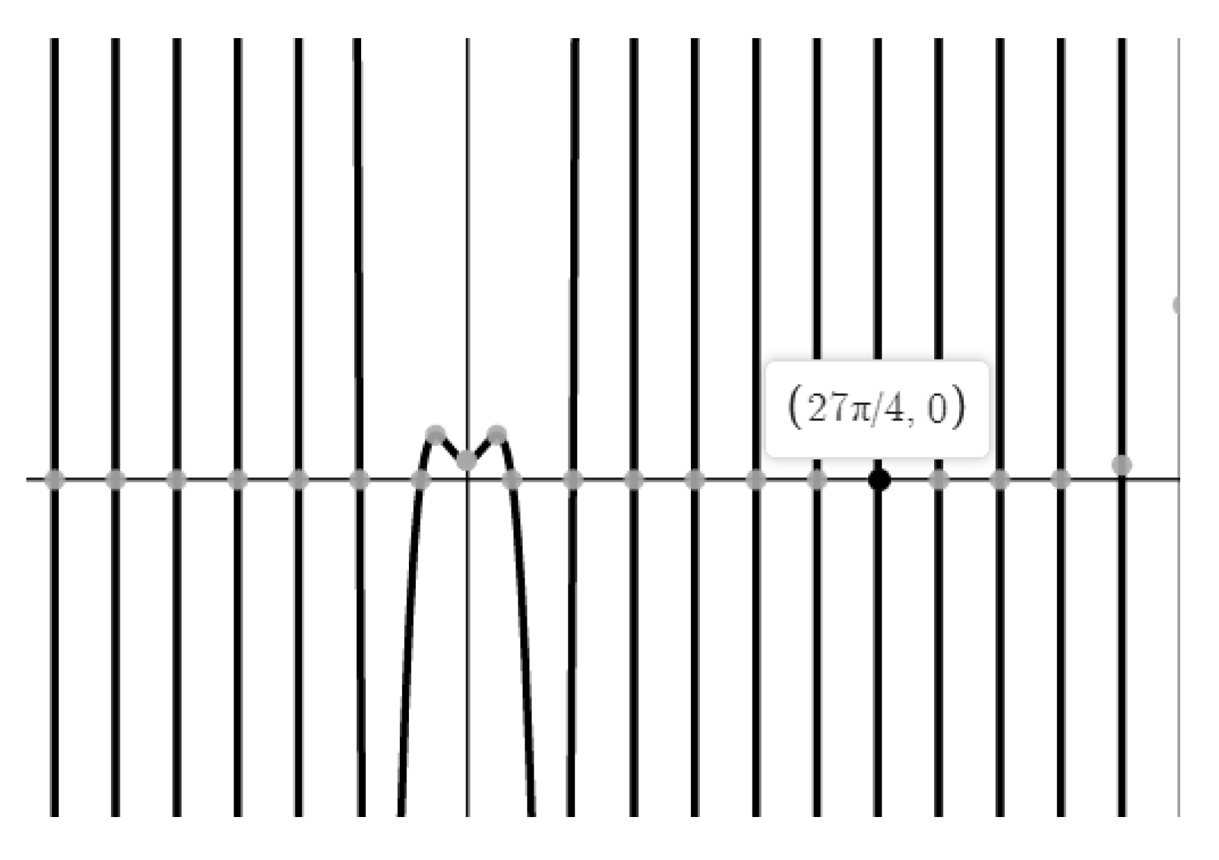
Theorem 6. Let , be the sequence of eigenvalues of the problem (1)–(9). Then has the following two asymptotic formulas: Proof. Since the eigenvalues of the problem is the zeros of the characteristic equation
by Theorem 4. Then from Equation (
36) we have,
Let
and
be the left and right side of Equation (
40). It is easy to show that
. Then by Rouch’s theorem
and
have the same number of zeros. The zeros of the function are near to
, for a sufficiently large integer
n, see
Figure 1. Hence we obtain (
38) and (
39). □
According to the asymptotic expressions of the fundamental system of solutions, eigenvalues and characteristic equation
. We evaluate asymptotic formulas for the eigenfunctions. Hence, the characteristic equation
is significant for estimating eigenvalues and eigenfunctions of the problem (
1)–(
9) (see [
14] (Theorem 4.1)).
Theorem 7. Asymptotic formulas for the eigenfunctions of the eigenvalue problem (1)–(9) corresponding to the eigenvalues has the following forms: Proof. From Equations (
23), (
25), (
31) and (
34) we can estimate
and
, then substituting these into the characteristic equation
. Hence, by a simple calculation, (
41) and (
42) can be obtained. □
Note that, from (
41) and (
42), we can verify that the formulas (
38) and (
39) are simple. In general, the eigenvalues of the problem (
1)–(
9) are simple (see [
9] (Theorem 4.2).
Example 1. If and , then Equation (1) reduced towith the conditions (2)–(9). In Reference [2], Şen investigated (43). He obtained asymptotic formulas for the fundamental solutions and eigenvalues for the problem. In this paper, we obtain an accurate asymptotic formulas for the eigenvalues for this problem. Substituting and into (38) and (39), then we have the following asymptotic formulas for the eigenvalues: Moreover, we show that the following formulas form asymptotic formulas for the eigenfunctions for Şen’s problem [2]: Example 2. We can note that in Equation (1), the weight functions and are constant functions on the intervals and respectively. In this example, we consider a special non constant real valued function: Since and and their derivatives are bounded on the intervals and , then from Equations (37) and (40), we obtain the following approximate expression for the eigenvalues of the problem:It is easy to show that Equations (41) and (42) are the eigenfunction for this particular case.


