An Enhanced Optimization Scheme Based on Gradient Descent Methods for Machine Learning

Abstract

A The learning process of machine learning consists of finding values of unknown weights in a cost function by minimizing the cost function based on learning data. However, since the cost function is not convex, it is conundrum to find the minimum value of the cost function. The existing methods used to find the minimum values usually use the first derivative of the cost function. When even the local minimum (but not a global minimum) is reached, since the first derivative of the cost function becomes zero, the methods give the local minimum values, so that the desired global minimum cannot be found. To overcome this problem, in this paper we modified one of the existing schemes—the adaptive momentum estimation scheme—by adding a new term, so that it can prevent the new optimizer from staying at local minimum. The convergence condition for the proposed scheme and the convergence value are also analyzed, and further explained through several numerical experiments whose cost function is non-convex.

1. Introduction

Deep learning is a part of a broader family of machine learning methods [1,2,3,4,5,6,7,8,9,10] based on learning data representations, as opposed to task-specific algorithms. Machine learning is a field of computer science that gives computer systems the ability to learn with data, without being explicitly programmed. In machine learning, a machine will find appropriate weight values of data by introducing a cost function. There are several optimization schemes [11,12,13,14,15,16,17,18,19,20,21,22,23,24,25] which can be used to find the weights by minimizing the cost function, such as the Gradient Descent method (GD) [26]. Also, there are many variations based on the GD method which can be used to improve the efficiency of the GD method. In particular, the adaptive momentum estimation (Adam) scheme [27,28] is the most popular scheme based on the GD. The Adam is constructed by computing individual adaptive learning rates for different parameters from estimates of first and second moments of the gradients. The Adam method has been widely used, and it is well-known that it is easy to implement, computationally efficient, and works quite well in most cases.

In this paper, we improve the Adam-based methods of finding the global minimum value of the non-convex cost function. In a typical Adam method, in order to find the minimum value of the cost function, the method looks for a value at which the first derivative of the cost function is zero, since the global minimum value is usually one of critical points. At a certain point, if the value falls to the local minimum, the value is not changed because the first derivative of the cost function is zero at the local minimum, and if the value of the cost function is greater than the expected value, then the value of the parameter has to be changed. Therefore, an additional value corresponding to the value of the cost function should be added to the part that changes the parameter. In other words, the existing Adam-based method makes use of only the first derivative of the cost function to make a parameter change, and sometimes it throws out one value of the local minimums, but not the global minimum value we want to find out.

Basically, the GD-based method, including Adam, has an assumption that the given cost function is convex, so a local minimum of the convex function is the desired global minimum. However, experiments and some facts have shown that many of cost functions are non-convex. Also, it is well-known that as the size of learning data increases through various experiences, the deep structure of the neural network becomes more difficult to learn. That is, the complexity of the neural network has a tendency to make the non-convex function. Therefore, a modified optimization scheme is required to find the global minimum for non-convex cost functions.

In this paper, for the non-convex cost functions, a new scheme proposes a modification of the classical Adam scheme—one variation of GD—to make a parameter change even at a local minimum by using the values of both the cost function and the first derivative of the cost function. Even though the parameter falls into a local minimum and the first derivative of the cost function is zero, the proposed method has a variation of the parameter depending on the value of the cost function. Therefore, the proposed method can get rid of that part, even if the parameter falls to a local minimum. Moreover, to show convergence of the proposed scheme, we prove that the proposed scheme satisfies the required convergence condition, and also present the limit of the convergence. Throughout several numerical tests, it is numerically shown that the proposed method is quite efficient compared to several existing optimization methods.

This paper is organized as follows: Firstly, we briefly explain the cost function in Section 2 and introduce the proposed scheme and its convergence analysis in Section 3. Numerical results are presented in Section 4 and we end up with the conclusion in Section 5.

2. Analysis of the Cost Function

In this section, we briefly review a cost function in machine learning. For this, we try to understand the principle of forming the structure with one neuron. Let x be an input data and H(x) be a output data, which is obtained by

$$\begin{array}{ccc}\hfill H\left(x\right)& =& \sigma (wx+b),\hfill \end{array}$$

(1)

where w is weight, b is bias, and $\sigma$ is a sigmoid function (universally called an activation function, and various functions can be used). Therefore, the result of the function H is made to be a value between 0 and 1, since H takes a continuous value. For machine learning, let $LS$ be the set of learning data, and let $l>2$ be the number of the size of $LS$. In other words, when the first departure point of learning data is 1, we can say that $LS=\{(x_1,y_1),(x_2,y_2),\dots ,(x_l,y_l)\}$, where $x_i$ is normalized during preprocessing and $y_i$∈$\{0,1\}$. From $LS$, we can define a cost function as follows:

$$\begin{array}{c}\hfill C(w,b)=\frac{1}{l}\sum _{s=1}^l{\left(y_s-H\left(x_s\right)\right)}^2.\end{array}$$

(2)

The machine learning is completed through w and b, which satisfy the minimum value of the cost function. Unfortunately, there may be several local minimum values of the cost function, when the cost function is not convex. Furthermore, if we extend the cost function with deep learning, the nature of convex is even harder to understand [13,15]. Note

$$\begin{array}{c}\hfill \left|\frac{\partial C}{\partial w}\right|\end{array}$$

(3)

is bounded by defining

$$\begin{array}{c}\hfill M=\frac{2}{l}\sum _{s=1}^l\left|x_s\right|,\end{array}$$

(4)

since

$$\begin{array}{ccc}\hfill \frac{\partial C}{\partial w}& =& -\frac{2}{l}\sum _{s=1}^l{x}_s\left(y_s-H\left(x_s\right)\right)H\left(x_s\right)\left(1-H\left(x_s\right)\right)\hfill \end{array}$$

(5)

$$\begin{array}{ccc}\hfill \left|\frac{\partial C}{\partial w}\right|& =& \frac{2}{l}\left|\sum _{s=1}^l{x}_s\left(y_s-H\left(x_s\right)\right)H\left(x_s\right)\left(1-H\left(x_s\right)\right)\right|\hfill \end{array}$$

(6)

$$\begin{array}{cc}\le & \frac{2}{l}\sum _{s=1}^l\left|x_s\right|\hfill \end{array}$$

(7)

$$\begin{array}{cc}=& M,\hfill \end{array}$$

(8)

where M is a positive real value.

2.1. Change of the Cost Function According to Learning Data

In this subsection, we show how the cost function is complicated according to learning data by showing how the number of local minima is increased. Note that the local minimum value means the lowest value in the neighborhood of a certain $x_s$.

Theorem 1.

In the cost function, when one learning data is received, the local minimum value can increase by one.

Proof. 

In order to find the convex properties, we need to calculate the second derivative of the cost function. The second derivative of the cost function is

$$\begin{array}{ccc}\hfill \frac{{\partial }^{2}C}{\partial w^2}& =& \frac{2}{l}\sum _{s=1}^l{\left(\frac{\partial H}{\partial w}\right)}^2-\frac{2}{l}\sum _{s=1}^l\left(y_s-H\left(x_s\right)\right)\frac{{\partial }^{2}H}{\partial w^2}\hfill \end{array}$$

(9)

$$\begin{array}{cc}=& \frac{2}{l}\sum _{s=1}^l{x}_s^2\left(H^2\left(w\right){\left(1-H\left(w\right)\right)}^2-\left(y_s-H\left(w\right)\right)H\left(w\right)\left(1-H\left(w\right)\right)\left(1-2H\left(w\right)\right)\right)\hfill \end{array}$$

(10)

$$\begin{array}{cc}=& \frac{2}{l}\sum _{s=1}^l{x}_s^2{g}_s\left(w\right),\hfill \end{array}$$

(11)

where $g_s=H_s(1-H_s)\left\{H_s(1-H_s)-(y_s-H_s)(1-2H_s)\right\}$ and $H_s=H\left(x_s\right)$. If $y_s$ = 0 for all s, then $x_s$ is negative, so $0<H_s<0.5$. Therefore, $g_s$ is positive in its domain ($0<H_s<0.5$) by the definition of $g_s$. The other case for $y_s$ = 1, for all s, has the same results. In both cases, where all $y_s$ has the same value, $g_s$ is always positive, so that the cost function is convex. Hence, we just check the other case, in which $y_s$ has different values for some s. For simplicity, we take $l=2$, then ${\sum }_{s=1}^l{x}_s^2{g}_s$ can be divided into two parts according to the $y_s$ value. When $y_1=1$, $\widehat{g}$ is $H_1(1-H_1)\left\{H_1(1-H_1)-(1-H_1)(1-2H_1)\right\}$ and when $y_2=0$, $\tilde{g}$ is $H_2(1-H_2)\left\{H_2(1-H_2)-(0-H_2)(1-2H_2)\right\}$. The cost function can be rewritten, such that

$$\begin{array}{c}\hfill \frac{{\partial }^{2}C}{\partial w^2}=x_1^2\widehat{g_1}+x_2^2\widetilde{g_2}.\end{array}$$

(12)

Assuming that $x_1>0$ and $x_2<0$, w satisfying the minimum of the cost function is ∞. The solutions of the equation $g_1=0$ are ${\sigma }^{-1}\left(0\right)/x_1-b$, ${\sigma }^{-1}(1/3)/x_1-b$, and ${\sigma }^{-1}\left(1\right)/x_1-b$. In particularly, the second derivative of the cost function, ${\partial }^{2}C/\partial w^2$ is negative on $[{\sigma }^{-1}\left(0\right)/x_1-b,{\sigma }^{-1}(1/3)/x_1-b]$. Similarly, the solution of the equation $g_2=0$ are ${\sigma }^{-1}\left(0\right)/x_2-b$, ${\sigma }^{-1}(2/3)/x_2-b$, and ${\sigma }^{-1}\left(1\right)/x_2-b$. The second derivative of the cost function, ${\partial }^{2}C/\partial w^2$ is negative on $[{\sigma }^{-1}\left(1\right)/x_2-b,{\sigma }^{-1}(2/3)/x_2-b]$. Thus, as the learning data grows, there is an increase in the interval where the second derivative of the cost function becomes negative. □

2.2. Change of the Cost Function According to Row

This method can be extended to a multi-neuron network [29,30]. For simplicity, a value of each neuron corresponds to a component of input data, so that the input data is represented as a vector. Let X be an input vector and $Y^k$ be an output vector at the kth hidden layer. From this, we can obtain

$$\begin{array}{ccc}\hfill Y^k=H^k\left(x\right)& =& \sigma (W^k{Y}^{k+1}+b^k),\hfill \end{array}$$

where $W^k$ and $b^k$ are a real matrix and real vector, respectively. Here, the calculation of the sigmoid function is done through composing each element of a vector. A vector $\zeta$ with m elements is calculated as follows:

$$\begin{array}{c}\hfill \sigma \left(\zeta \right)=\left(\begin{array}{c}\sigma \left({\zeta }_1\right)\\ \sigma \left({\zeta }_2\right)\\ ⋮\\ \sigma \left({\zeta }_m\right)\end{array}\right).\end{array}$$

If $\partial C/\partial {\zeta }_i$ is non-convex, then $\partial C/\partial \zeta$ is also non-convex.

3. Dynamic Adaptive Momentum Method

The main idea starts with a fixed-point iteration method [26] and the condition of the cost function ($0\le C(w,b)$). Since the cost function is lower-bounded and continuous on [0, 1], we can find a minimizer $(w^{*},b^{*})$, such that $C(w^{*},b^{*})\le C(w,b)$ for all $(w,b)$. Note that w and b are the initial conditions which are randomly selected from the normal distribution.

3.1. Adam

Before describing the new scheme, we will briefly review the Adam scheme since the new scheme is a modification of the Adam. The Adam is defined as follows:

$$\begin{array}{ccc}\hfill w_{i+1}& =& w_i-\eta \frac{{\widehat{m}}_i}{\sqrt{\widehat{v_i}+ϵ}},\hfill \end{array}$$

(13)

where

$$\begin{array}{ccc}\hfill m_i& =& {\beta }_1{m}_{i-1}+(1-{\beta }_1)\frac{\partial C\left(w_i\right)}{\partial w},\hfill \end{array}$$

(14)

$$\begin{array}{ccc}\hfill v_i& =& {\beta }_2{v}_{i-1}+(1-{\beta }_2){\left(\frac{\partial C\left(w_i\right)}{\partial w}\right)}^2,\hfill \end{array}$$

(15)

$$\begin{array}{ccc}\hfill {\widehat{m}}_i& =& m_i/(1-{\beta }_1),{\widehat{v}}_i=v_i/(1-{\beta }_2).\hfill \end{array}$$

(16)

It is well-known that Adam works well for convex cost functions. Note that $\frac{\partial C\left(w_i\right)}{\partial w}$ is usually zero at the local and global minimum points. Hence, at even local minima, $\frac{\partial C\left(w_i\right)}{\partial w}$ is close to zero, so that $m_i$ and $v_i$ can be zero and $w_i$ can converge. To hurdle this drawback, the modification of Adam is required for a non-convex cost function.

3.2. Dynamic Adaptive Momentum Method

In this subsection, we show how the Adam scheme can be modified for a non-convex cost function. The basic form of the new scheme is quite similar to that of the Adam. In the proposed scheme, the new term $\lambda tanh\left(C\left(w_i\right)\right)$ is added to the Adam formula to prevent it from staying as local minima.

The proposed formula is defined as follows:

$$\begin{array}{ccc}\hfill w_{i+1}& =& w_i-\eta \frac{{\widehat{m}}_i}{\sqrt{\widehat{v_i}+ϵ}}+\lambda tanh\left(C\left(w_i\right)\right),\hfill \end{array}$$

(17)

where

$$\begin{array}{ccc}\hfill \lambda & =& -\frac{sign\left(\frac{\partial C\left(w_i\right)}{\partial w}\right)}{M}\hfill \end{array}$$

(18)

$$\begin{array}{ccc}\hfill m_i& =& {\beta }_1{m}_{i-1}+(1-{\beta }_1)\frac{\partial C\left(w_i\right)}{\partial w},\hfill \end{array}$$

(19)

$$\begin{array}{ccc}\hfill v_i& =& {\beta }_2{v}_{i-1}+(1-{\beta }_2){\left(\frac{\partial C\left(w_i\right)}{\partial w}\right)}^2,\hfill \end{array}$$

(20)

$$\begin{array}{ccc}\hfill {\widehat{m}}_i& =& m_i/(1-{\beta }_1),{\widehat{v}}_i=v_i/(1-{\beta }_2).\hfill \end{array}$$

(21)

The Equation (18) can be changed as

$$\begin{array}{ccc}\hfill m_i& =& {\beta }_1^i{m}_0+(1-{\beta }_1)\sum _{k=1}^i{\beta }_1^{k-1}\frac{\partial C\left(w_{i-k+1}\right)}{\partial w}\hfill \end{array}$$

(22)

$$\begin{array}{cc}=& (1-{\beta }_1)\sum _{k=1}^i{\beta }_1^{k-1}\frac{\partial C\left(w_{i-k+1}\right)}{\partial w}\hfill \end{array}$$

(23)

$$\begin{array}{ccc}\hfill v_i& =& {\beta }_2^i{v}_0+(1-{\beta }_2)\sum _{k=1}^i{\beta }_2^{k-1}{\left(\frac{\partial C\left(w_{i-k+1}\right)}{\partial w}\right)}^2\hfill \end{array}$$

(24)

$$\begin{array}{cc}=& (1-{\beta }_2)\sum _{k=1}^i{\beta }_2^{k-1}{\left(\frac{\partial C\left(w_{i-k+1}\right)}{\partial w}\right)}^2,\hfill \end{array}$$

(25)

with assumptions $m_0=0$ and $v_0=0$. Therefore, the Equation (17) can be changed as

$$\begin{array}{ccc}\hfill w_{i+1}& =& w_i-\eta \frac{\sqrt{1-{\beta }_2}}{1-{\beta }_1}\frac{(1-{\beta }_1){\sum }_{k=1}^i{\beta }_1^{k-1}\frac{\partial C\left(w_{i-k+1}\right)}{\partial w}}{\sqrt{(1-{\beta }_2){\sum }_{k=1}^i{\beta }_2^{k-1}{\left(\frac{\partial C\left(w_{i-k+1}\right)}{\partial w}\right)}^2+ϵ}}+\lambda tanh\left(C\left(w_i\right)\right)\hfill \\ & =& w_i-\eta \frac{{\sum }_{k=1}^i{\beta }_1^{k-1}\frac{\partial C\left(w_{i-k+1}\right)}{\partial w}}{\sqrt{{\sum }_{k=1}^i{\beta }_2^{k-1}{\left(\frac{\partial C\left(w_{i-k+1}\right)}{\partial w}\right)}^2+ϵ}}+\lambda tanh\left(C\left(w_i\right)\right)\hfill \end{array}$$

$$\begin{array}{cc}=& w_i-\eta \frac{S_i}{\sqrt{S{S}_i+ϵ}}+\lambda tanh\left(C\left(w_i\right)\right)\hfill \end{array}$$

(26)

$$\begin{array}{cc}=& g\left(w\right),\hfill \end{array}$$

(27)

where

$$\begin{array}{ccc}\hfill S_i& =& \sum _{k=1}^i{\beta }_1^{k-1}\frac{\partial C\left(w_{i-k}\right)}{\partial w},S{S}_i=\sum _{k=1}^i{\beta }_2^{k-1}{\left(\frac{\partial C\left(w_{i-k}\right)}{\partial w}\right)}^2,\hfill \end{array}$$

(28)

$$\begin{array}{cc}\hfill \mathrm{and}& g\left(w\right)=w+\lambda tanh\left(C\left(w\right)\right)-\eta \frac{S_i}{\sqrt{S{S}_i+ϵ}}.\hfill \end{array}$$

(29)

Here, we look for the convergence condition of the proposed iteration scheme. The iteration scheme is simply represented by

$$\begin{array}{c}\hfill w_{i+1}=g\left(w_i\right).\end{array}$$

(30)

Since $i>\tau$ ($\tau$ is a sufficiently large integer), we have

$$\begin{array}{c}\hfill \left|w_{i+1}-w_i\right|=\left|g\left(w_i\right)-g\left(w_{i-1}\right)\right|\le \left|\frac{\partial g\left(\zeta \right)}{\partial w}\right|\left|w_i-w_{i-1}\right|,\end{array}$$

(31)

where $\zeta$ is between $w_{i-1}$ and $w_i$. By letting $\nu =\partial g/\partial w$, we can eventually have

$$|w_{i+1}-w_i|\le {\nu }^{i-\tau }|w_{\tau +1}-w_{\tau }|.$$

(32)

As the iteration continues, the value of ${\nu }^{i-\tau }$ converges to zero if $|\partial g/\partial w|<1$. Therefore, after a sufficiently large number (greater than $\tau$), $w_{i+1}$ and $w_i$ are equal. Assuming that $|\partial g(w)/\partial w|=\nu <1$, the sequence $\left\{w_i\right\}$ is a cauchy sequence, so that it can be convergent [31]. Therefore, we need to check that the proposed method satisfies the convergence condition $|\partial g(w)/\partial w|<1$.

Theorem 2.

The proposed method satisfies the convergence condition $|\partial g(w)/\partial w|<1$.

Proof. 

In order to satisfy the convergence condition, we should compute the equation:

$$\begin{array}{ccc}\hfill \frac{\partial g}{\partial w}& =& 1+\lambda \frac{\partial tanh\left(C\right)}{\partial w}-\eta \frac{{\partial }^{2}C}{\partial w^2}\left(\frac{{\beta }_{2}S{S}_{i-1}-{\beta }_1{S}_{i-1}\frac{\partial C}{\partial w}}{{\left({\left(\frac{\partial C}{\partial w}\right)}^2+{\beta }_{2}S{S}_{i-1}\right)}^{3/2}}\right)+\frac{\partial \lambda }{\partial w}tanh\left(C\right)\hfill \end{array}$$

(33)

$$\begin{array}{cc}=& 1+\lambda \left(1-{\left(tanh\left(C\right)\right)}^2\right)\frac{\partial C}{\partial w}-\eta \frac{{\partial }^{2}C}{\partial w^2}\left(\frac{{\beta }_2-{\beta }_1\frac{S_{i-1}}{S{S}_{i-1}}\frac{\partial C}{\partial w}}{{\left({\left(\frac{1}{S{S}_{i-1}}\frac{\partial C}{\partial w}\right)}^2+{\beta }_2\right)}^{3/2}}\right)\frac{1}{S{S}_{i-1}^{1/2}},\hfill \end{array}$$

(34)

because $\partial \lambda /\partial w$ is 0 almost everywhere.

Since ${\beta }_2\approx 1$, $\eta$ is a sufficiently small number and $i>\tau$ ($\tau$ is a sufficiently large integer), we have

$$\begin{array}{ccc}\hfill \eta \frac{{\partial }^{2}C}{\partial w^2}\left(\frac{{\beta }_2-{\beta }_1\frac{S_{i-1}}{S{S}_{i-1}}\frac{\partial C}{\partial w}}{{\left({\left(\frac{1}{S{S}_{i-1}}\frac{\partial C}{\partial w}\right)}^2+{\beta }_2\right)}^{3/2}}\right)\frac{1}{S{S}_{i-1}^{1/2}}& \approx & 0,\hfill \end{array}$$

(35)

and

$$\begin{array}{ccc}\hfill \frac{\partial g}{\partial w}=1+\lambda \left(1-{\left(tanh\left(C\right)\right)}^2\right)\frac{\partial C}{\partial w}& =& 1-\left(1-{\left(tanh\left(C\right)\right)}^2\right)\frac{\left|\frac{\partial C}{\partial w}\right|}{M}.\hfill \end{array}$$

(36)

Therefore, $|\partial g(w)/\partial w|<1$. □

Since the sequence defined in the proposed scheme converges, the limit of the convergence can be represented as follows:

Theorem 3.

The limit of the parameter, $w^{*}$, in the proposed method satisfies

$$C\left(w^{*}\right)\approx {tanh}^{-1}\left(\eta max\left\{\frac{\partial C\left(w\right)}{\partial w}\right\}\frac{{(1-{\beta }_2)}^{1/2}}{1-{\beta }_1}\right).$$

Proof. 

After a sufficiently large number (greater than $\tau$), we have $w^{*}=g\left(w^{*}\right)$. After computing

$$\begin{array}{ccc}\hfill \lambda tanh\left(C\left(w^{*}\right)\right)& -& \eta \frac{S_{*}}{\sqrt{S{S}_{*}+ϵ}}=0\hfill \end{array}$$

(37)

and

$$\begin{array}{cc}\hfill S_{*}\approx \frac{\partial C\left(w^{*}\right)}{\partial w}\frac{1}{1-{\beta }_1},& S{S}_{*}\approx {\left(\frac{\partial C\left(w^{*}\right)}{\partial w}\right)}^2\frac{1}{1-{\beta }_2},\hfill \end{array}$$

(38)

one can have the following equations,

$$\begin{array}{ccc}\hfill \lambda tanh\left(C\left(w^{*}\right)\right)& -& \eta sign\left(\frac{\partial C}{\partial w}\right)\frac{{(1-{\beta }_2)}^{1/2}}{1-{\beta }_1}\approx 0\hfill \end{array}$$

(39)

$$\begin{array}{ccc}\hfill tanh\left(C\left(w^{*}\right)\right)& \approx & \eta M\left(\frac{{(1-{\beta }_2)}^{1/2}}{1-{\beta }_1}\right)\hfill \end{array}$$

(40)

$$\begin{array}{ccc}\hfill C\left(w^{*}\right)& \approx & {tanh}^{-1}\left(\eta M\frac{{(1-{\beta }_2)}^{1/2}}{1-{\beta }_1}\right).\hfill \end{array}$$

(41)

 □

4. Numerical Tests

In this section, several numerical experiments are presented to show the superiority of the proposed method by comparing numerical results obtained from the proposed scheme with results from other existing schemes, such as GD, Adam, and AdaMax for a non-convex function. Note that AdaMax [27] is one of the variants of Adam optimization schemes based on the infinity norm, where it is known that it is more suitable for sparsely updated parameters.

4.1. Classification

As the first example, we test a classification problem to distinguish a positive value and a negative value. That is, if the input value is positive, then the output is 1; and if the input is negative, the output is 0. For the experiment, the learning data set (LS) is simply given as $LS=\left\{\right(5,1),(-2,0),(50,1),(-0.2,1\left)\right\}$.

To examine a convergence property of the proposed optimization scheme in terms of the number of layers, we test the proposed method by varying the number of layers (three and five layers). Note that the initial weights are randomly provided. For the three layers case, the initial values are randomly selected $b_1=b_2=b_3=0$, $w_1=0.19771976$, $w_2=0.15725612$, and $w_3=-0.28434913$ and the number of iteration is 100. The GD only uses 1000 iterations due to slow learning speed. For the five layers case, the initial value is fixed to $b_1=b_2=b_3=b_4=b_5=0$, $w_1=0.34004834$, $w_2=1.09908653$, $w_3=-0.38793867$, $w_4=-1.48041442$, and $w_5=-0.74076256$, and the number of iteration is 100. Other parameters are provided in

Table 1. Initial parameters.

Method	Learning Rate	Parameters
GD	0.8
Adam	0.5	${\beta }_1=0.9,{\beta }_2=0.999,ϵ={10}^{-8}$
AdaMax	0.5	${\beta }_1=0.9,{\beta }_2=0.999$
Proposed	0.5	${\beta }_1=0.9,{\beta }_2=0.999,M=10$

.

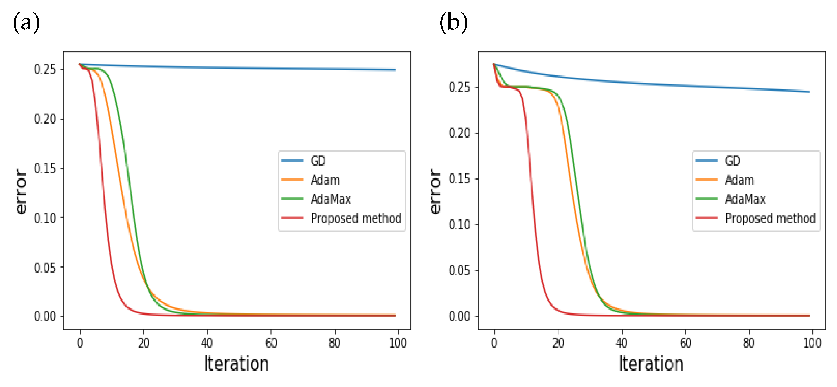
Based on the initial parameters, the numerical results for the three- and five-layer cases are plotted in Figure 1a,b, respectively.

Figure 1a,b present the convergence behavior of the proposed and existing schemes (GD, Adam, AdaMax) according to iterations. As seen in the Figures, the errors of the proposed scheme decrease much faster than others for both the three- and five-layer cases. Note that GD is not even close to zero.

4.2. One Variable Non-Convex Function Test

For the second example, we investigate behaviors of the proposed optimization for a non-convex cost function. A cost function in this experiment is assumed to be a non-convex function,

$$C\left(w\right)=\frac{(w+5)(w+3)(w-1)(w-10)}{800}+3.$$

(42)

Note that the global minimum of the given cost function is located at $w=7.1047$. The starting point is $w=-9$ and the iteration number is 100. Note that the blue line in the numerical results (Figure 2) represents a graph of the cost function $C\left(w\right)$ according to the change of w. Ohter initial conditions of the proposed and other existing schemes are given in

Table 2. Initial parameters.

Method	Learning Rate	Parameters
GD	0.2
Adam	0.2	${\beta }_1=0.9,{\beta }_2=0.999,ϵ={10}^{-8}$
AdaMax	0.2	${\beta }_1=0.9,{\beta }_2=0.999$
Proposed	0.2	${\beta }_1=0.9,{\beta }_2=0.999,M=100$

.

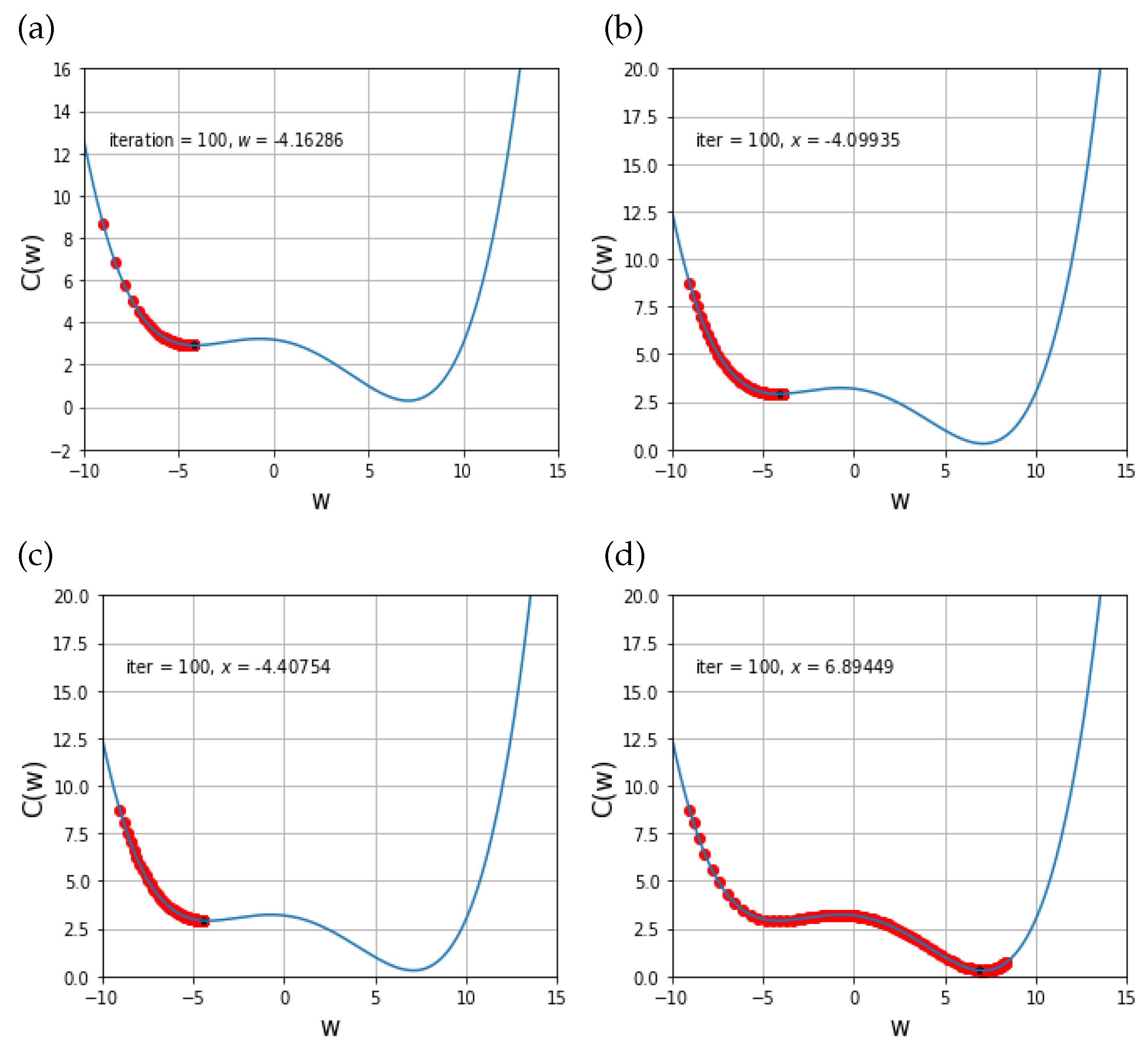
Based on the given initial conditions, we plot the solution behaviors of the proposed scheme with respect to the value of w, and plot those of the other existing schemes for comparisons in Figure 2. Notice that the given cost function has two local minimum points and one of these is the global minimum point, which is a final value from this experiment.

Figure 2d shows the numerical results obtained from the proposed scheme, and one can see that this scheme can find the global minimum points after 100 iteration times. However, other results seen in Figure 2a–c shows that solution behaviors of GD, Adam, AdaMax just stop at a local minimum, but not the global minimum point. Notice that even more iterations cannot help to find the global minimum.

4.3. One Variable Non-Convex Function Test: Local Minimums Exist in Three Places

For further investigation of the solution behaviors, we test a more complicated case, which has three local minimum points. The cost function in this experiment is set to

$$C\left(w\right)=\frac{(w+8)(w+6)(w+1)(w-2)(w-5)(w-12)}{50000}+5.2.$$

(43)

The starting point is −9, and the iteration number is 100. Also, the global minimum is located at $w=10.1$. Similar to the above, the blue line in the results represents the cost function $C\left(w\right)$ according to the change of w.

Table 3. Initial parameters.

Method	Learning Rate	Parameters
GD	0.2
Adam	0.2	${\beta }_1=0.9,{\beta }_2=0.999,ϵ={10}^{-8}$
AdaMax	0.2	${\beta }_1=0.9,{\beta }_2=0.999$
Proposed	0.2	${\beta }_1=0.9,{\beta }_2=0.999,M=100$

provides the initial parameters required in the proposed scheme, as well as the other existing schemes.

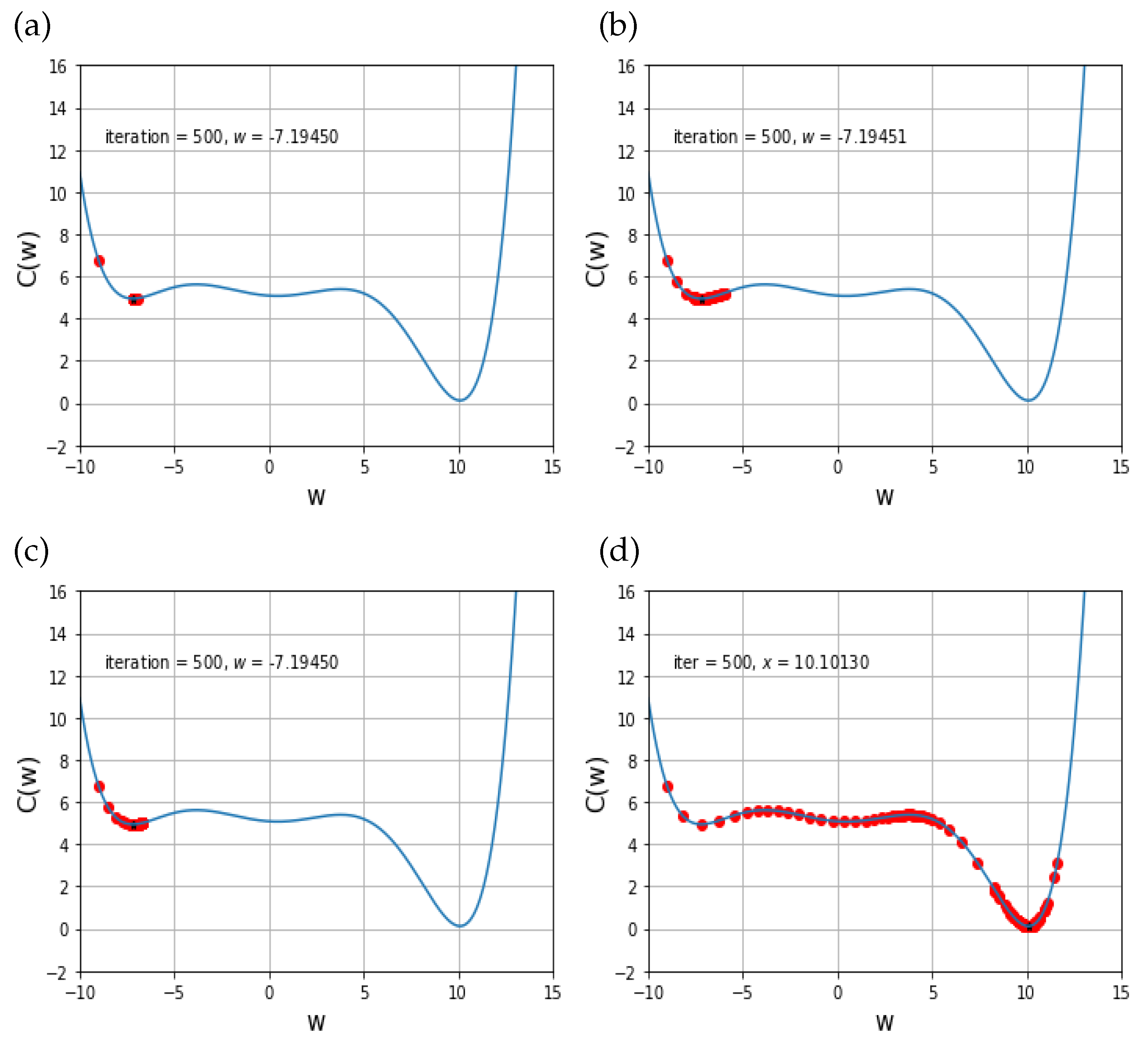
Based on the given initial conditions, the solution behaviors of the proposed scheme were plotted and compared with those of the other existing schemes in Figure 3. In this experiment, the given cost function has three local minimum points, and the final local point is the global minimum point.

From the Figure 3a–d, one can see that the proposed scheme can find the global minimum points after 100 iteration times, whereas the solution behaviors of GD, Adam, and AdaMax just stay at a local minimum, but not the global minimum point. Also, Figure 3a–c show that the other schemes cannot pass the first local minimum once they meet the first local minimum. Hence, one can conclude that the proposed scheme is able to distinguish between the global minimum and non-global local minima, which is a main contribution of this work.

4.4. Two-Dimensional Non-Convex BEALE Function

In the fourth experiment, we examined the solution behavior of the proposed optimization scheme for a two-dimensional case. The cost function in this experiment is defined as

$$C(w_1,w_2)={(1.5-w_1+w_1{w}_2)}^2+{(2.25-w_1+w_1{w}_2^2)}^2+{(2.625-w_1+w_1{w}_2^3)}^2,$$

(44)

and has the global minimum at $(w_1,w_2)=(3,0.5)$. An initial point starts at $(2,2)$ and the iteration number is 300. Similar to the above, the initial parameters for the proposed scheme and other existing schemes are shown in

Table 4. Initial parameters.

Method	Learning Rate	Parameters
GD	${10}^{-4}$
Adam	${10}^{-1}$	${\beta }_1=0.9,{\beta }_2=0.999,ϵ={10}^{-8}$
AdaMax	${10}^{-1}$	${\beta }_1=0.9,{\beta }_2=0.999$
Proposed	${10}^{-1}$	${\beta }_1=0.9,{\beta }_2=0.999,M=100$

.

Based on these initial conditions, the numerical results are plotted in Figure 4. Note that the initial point $(2,2)$ is quite close to the desired point, $(3,0.5)$.

Figure 4 shows that all methods converge well because the given cost function is convex around the given starting point.

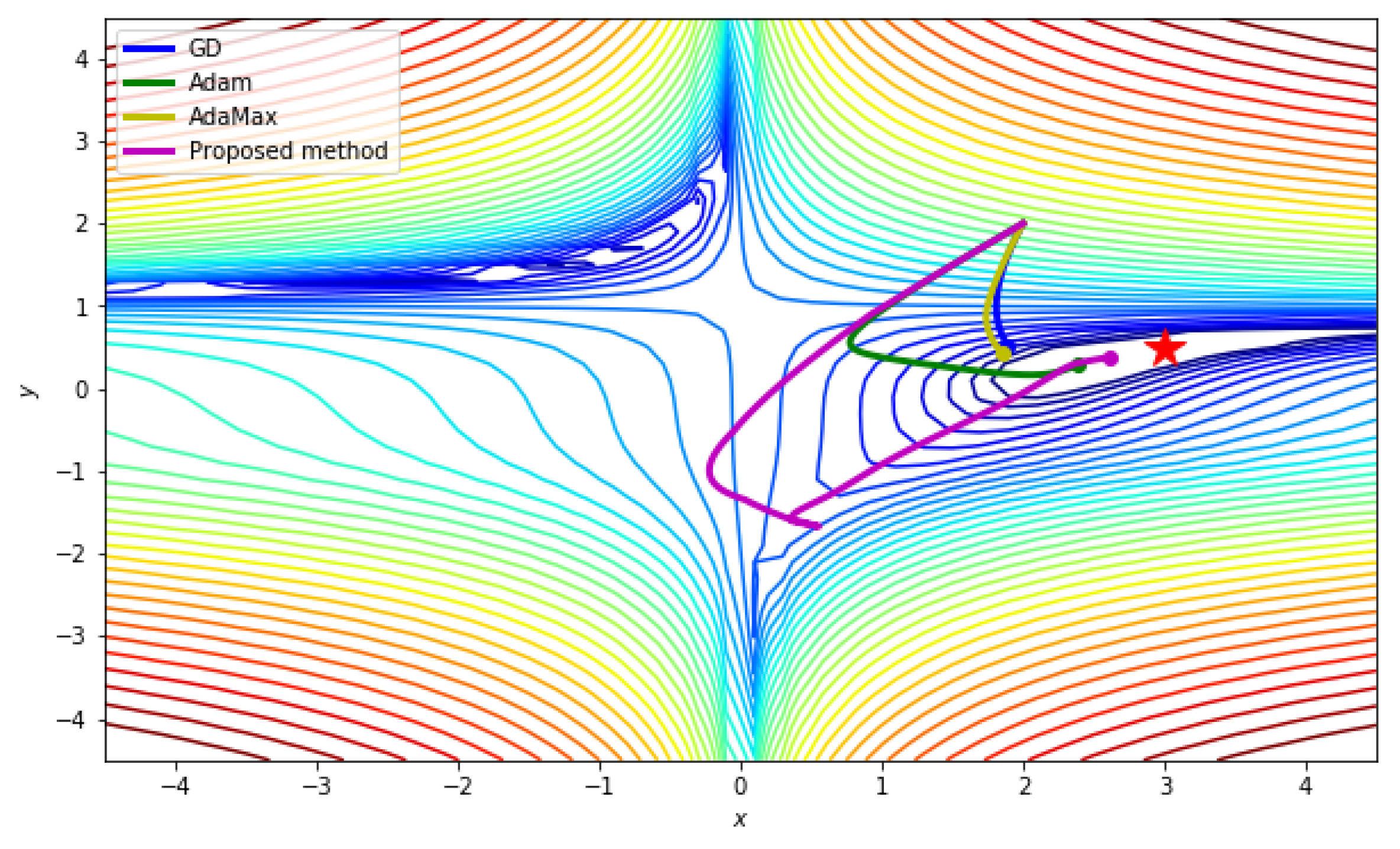
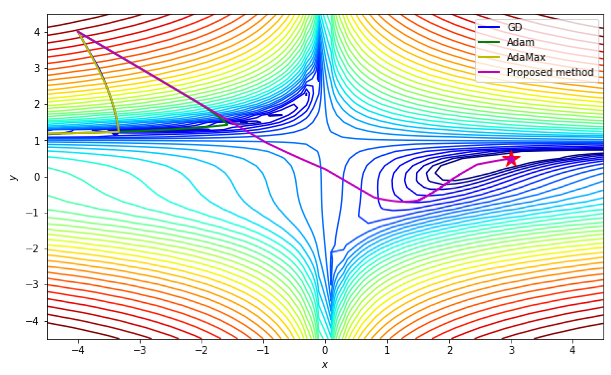
In order to investigate the effect of the initial points, we tested the same cost function with a different starting point $(w_1,w_2)=(-4,4)$, and the iteration number was set to 50,000 with the same initial parameters defined in Table 4. However, unlike the previous case, the starting point is far from the global minimum point in the given cost function, and a region between the starting point and the global minimum contains non-convex parts of the cost function.

Figure 5 presents the numerical results. Note that the given cost function is non-convex around the starting point (−4, 4). The numerical result in Figure 5 shows that GD, Adam, and AdaMax fall into a local minimum and stop there, whereas the proposed scheme reaches the global minimum.

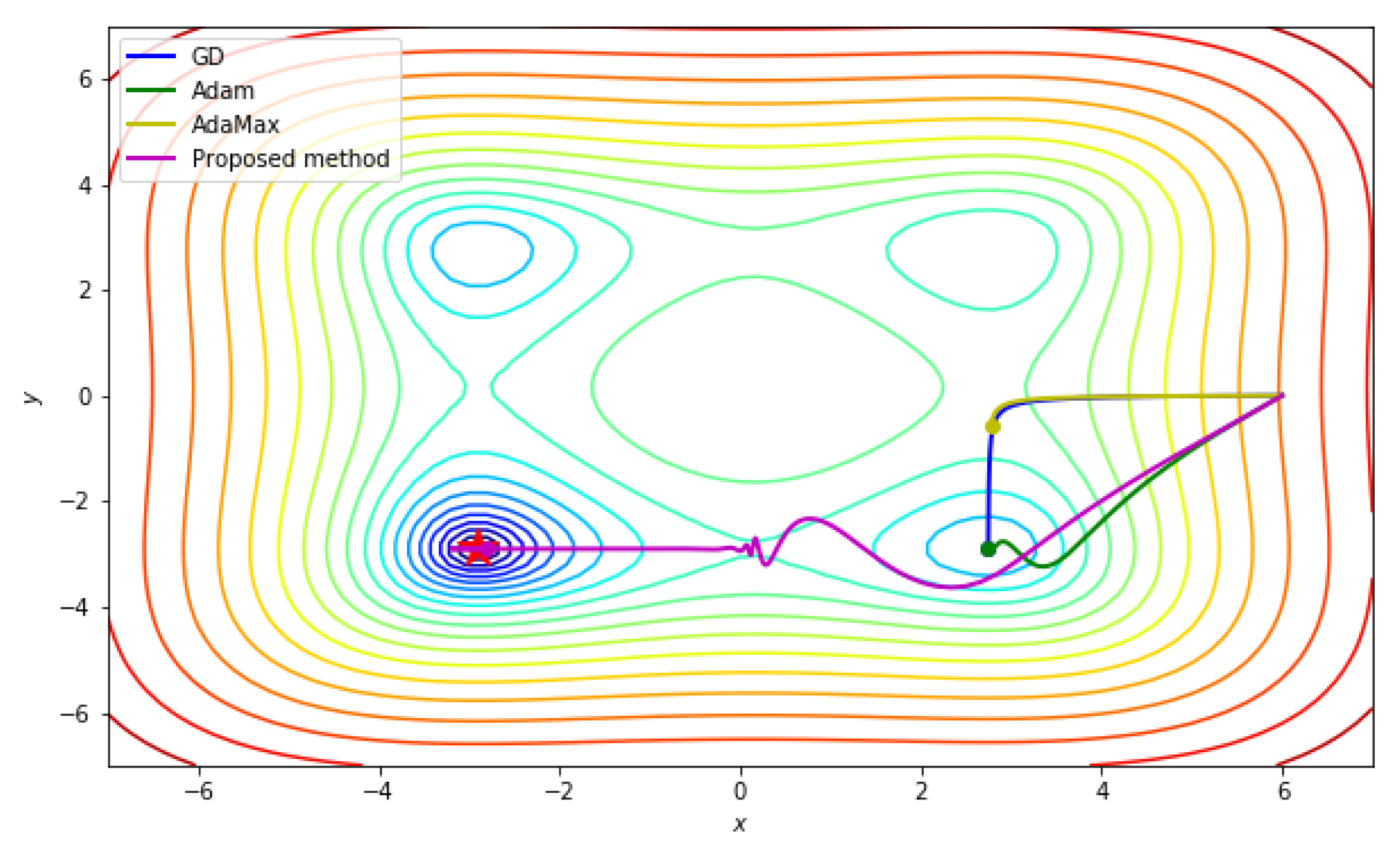
4.5. Two Variables Non-Convex Stybliski-Tang Function

In this next experiment we tested a more complicated case, where the cost function is defined as

$$C(w_1,w_2)=((w_1^4-16w_1^2+5w_1)+(w_2^4-16w_2^2+5w_2))/2+80.$$

(45)

The global minimum is located at $(w_1,w_2)=(-2.903534,-2.903534)$. For the test, a starting point $(w_1,w_2)=(6,0)$ was set to be far from the global minimum, and the iteration number was set to 300. The other initial parameters were set as seen in

Table 5. Initial parameters.

Method	Learning Rate	Parameters
GD	${10}^{-4}$
Adam	${10}^{-1}$	${\beta }_1=0.9,{\beta }_2=0.999,ϵ={10}^{-8}$
AdaMax	${10}^{-1}$	${\beta }_1=0.9,{\beta }_2=0.999$
Proposed	${10}^{-1}$	${\beta }_1=0.9,{\beta }_2=0.999,M=2000$

.

Based on the initial parameters, we checked the solution behavior of the proposed scheme and other existing ones for comparison in Figure 6.

Figure 6 shows that the proposed scheme can only converge to the desired point, whereas other schemes cannot converge. Note that the given cost function is non-convex near the starting point (6, 0).

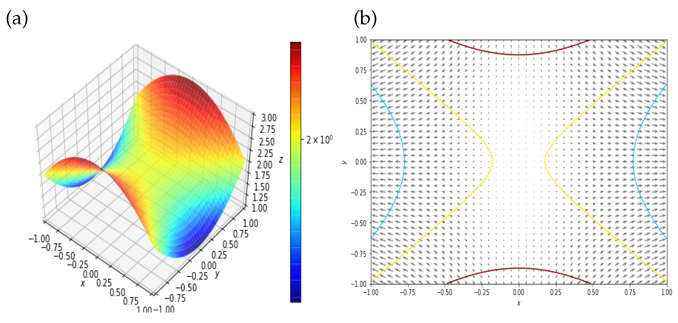
4.6. Two-Dimensional Non-Convex Function Having Saddle Point

Basically, the optimization schemes find the global minimum of a given cost function, and the global minimum point is usually the lowest of the critical points. However, we cannot guarantee that all global minimums are one of the critical points. The typical two-dimensional example is a function which has saddle points.

Hence, to examine the convergence behavior of the optimization scheme in this case, we set up the cost function as $C(w_1,w_2)=w_2^2-w_1^2+2$ whose hessian matrix is $\left(\begin{array}{cc}-2& 0\\ 0& 2\end{array}\right)$, so the function has a saddle point for every point in its own domain. The function is plotted in Figure 7.

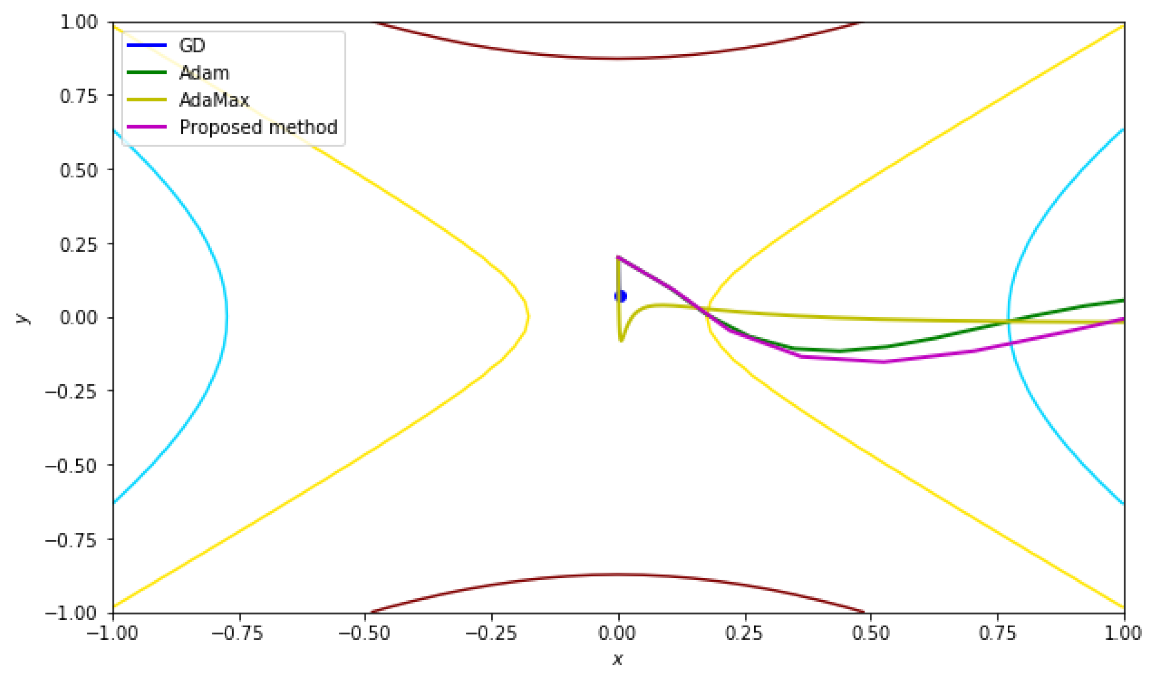
For the test, we set up the starting point at (0, 0.01) and the iteration number was 100. Other parameters are shown in

Table 6. Initial parameters.

Method	Learning Rate	Parameters
GD	${10}^{-3}$
Adam	${10}^{-1}$	${\beta }_1=0.9,{\beta }_2=0.999,ϵ={10}^{-8}$
AdaMax	${10}^{-1}$	${\beta }_1=0.9,{\beta }_2=0.999$
Proposed	${10}^{-1}$	${\beta }_1=0.95,{\beta }_2=0.999,M=100$

.

Similarly to the above, based on these initial parameters, we tested the proposed scheme and other existing schemes. Note that the cost function in this test has a saddle point, so we expected to find the smallest value of the whole domain.

Results are shown in Figure 8.

The numerical result plotted in Figure 8 shows that only the proposed scheme can converge to the desired point, whereas the other existing schemes cannot.

4.7. Fuzzy Model: Probability of Precipitation

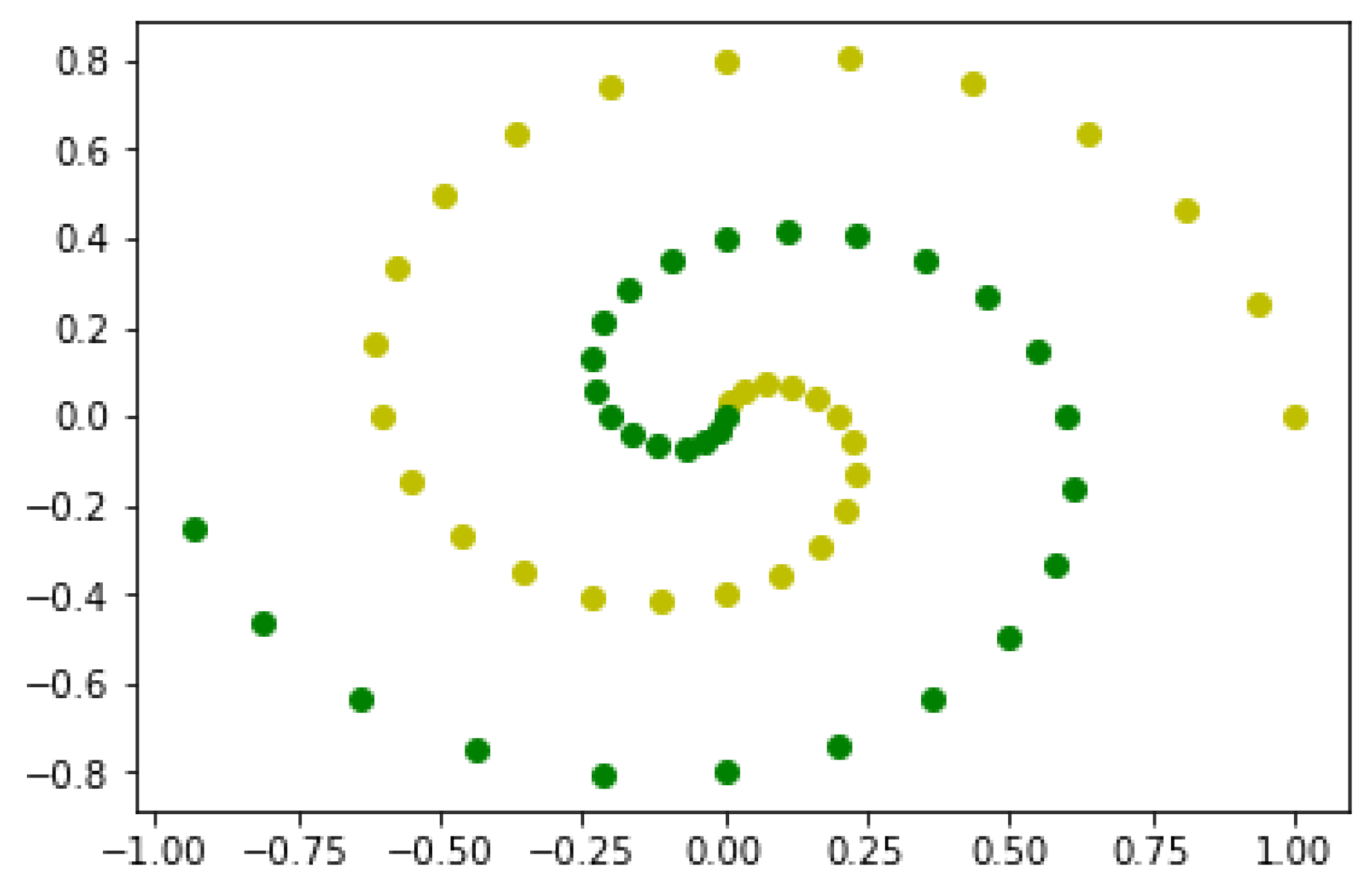
As mentioned, the proposed scheme can also be applied to the fuzzy model system, so we tried to apply the scheme to predict the probability of rain based on the given data.

Figure 9 represents given data for the current precipitation. Light-green dots represent zero probability of rain at the region, and dark-green dots represent data points where it is currently raining.

The cost function is defined by

$$C(w,b)=\frac{1}{l}\sum _{s=1}^l{(y_s-H\left(x_s\right))}^2,$$

(46)

where $H\left(x_s\right)=\sigma (w{x}_s+b)$, $\sigma$ is a sigmoidal function and $x_s$ is a point in xy-plane. The initial values of parameters used in this test are presented in

Table 7. Initial parameters.

Method	Learning Rate	Parameters
GD	${10}^{-2}$
Adam	${10}^{-2}$	${\beta }_1=0.9,{\beta }_2=0.999,ϵ={10}^{-8}$
AdaMax	${10}^{-2}$	${\beta }_1=0.9,{\beta }_2=0.999$
Proposed	${10}^{-2}$	${\beta }_1=0.95,{\beta }_2=0.999,M=100$

.

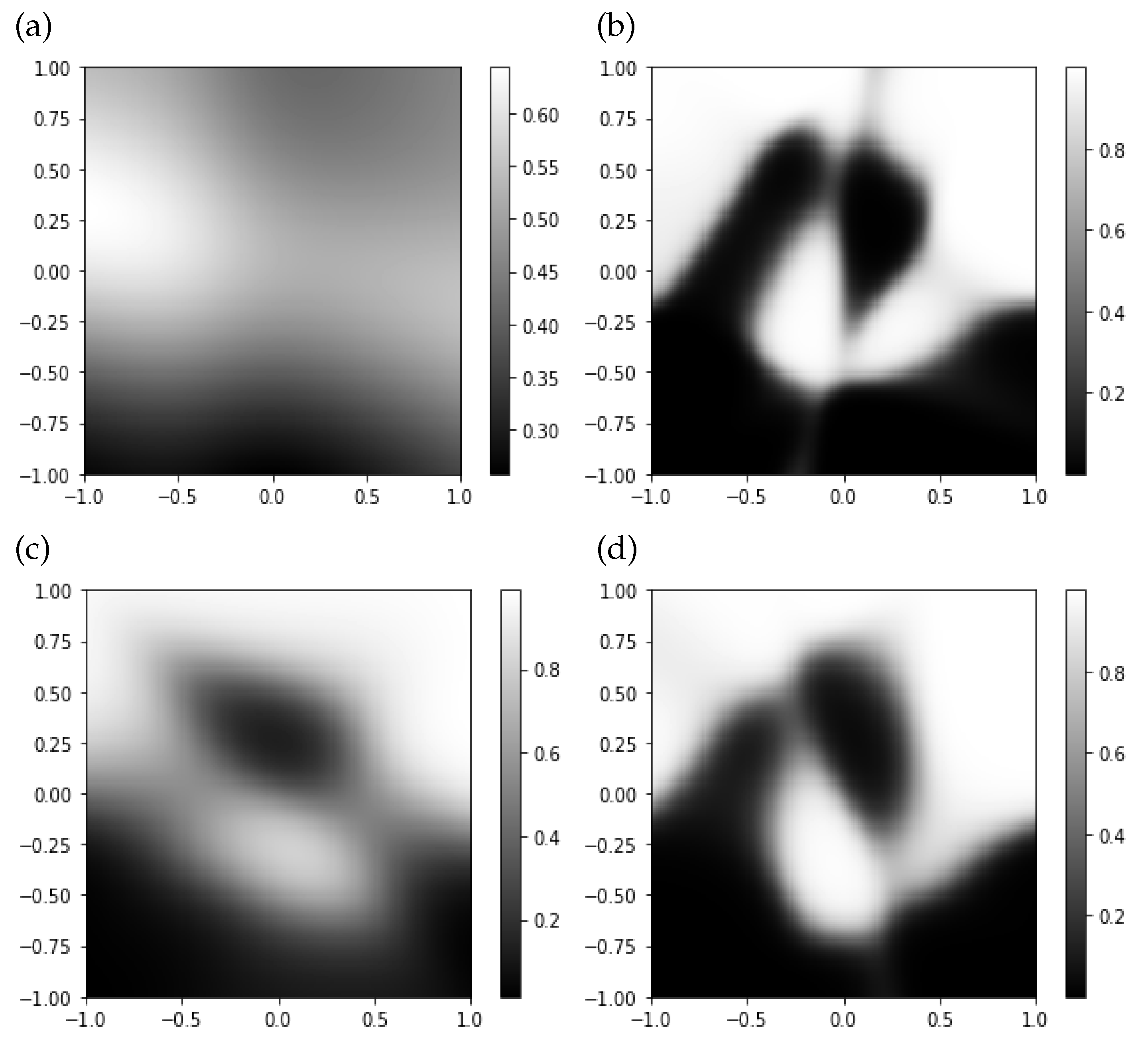
The numerical results induced from the proposed optimization scheme is plotted in Figure 10 and compared with results obtained from the existing schemes—GD, Adam, and AdaMax.

One can see that a result from the proposed algorithm gives more reasonable phenomena for the probability of precipitation, whereas the other existing schemes generate very ambiguous results, especially those from GD and AdaMax.

5. Conclusions

In this paper, we introduced an enhanced optimization scheme based on the popular optimization scheme, Adam, for non-convex problems induced from the machine learning process. Most existing optimizers may stay at a local minimum for non-convex problems when they meet the local minimum before meeting a global minimum. Even they have some difficulty in finding the global minimum within a complicated non-convex system. To prevent such phenomena, the classical Adam formula was modified by adding a new term with a non-negligible value at the local minimums, making it become zero at the global minimum. Hence, the modified optimizer never converges at local minimum points, and it can only converge at the global minimum.

Additionally, a convergence condition required in the proposed scheme was explained, and the limit of convergence was also provided. Throughout several numerical experiments, one could see that other existing methods did not converge to the desired point for critical initial conditions, whereas the proposed scheme could reach the global minimum point. Therefore, one can conclude that the proposed scheme performs very well compared with other existing schemes, such as GD, Adam, and AdaMax. Currently, we are investigating the generalization of the proposed scheme for deep-layer and multi-variable cases, which are the limitations of the current work. The preliminary results are quite promising, and we plan to report these soon.

References

- Dean, J.; Corrado, G.; Monga, R.; Chen, K.; Devin, M.; Le, Q.; Mao, M.; Ranzato, M.; Senior, A.; Tucker, P.; et al. Large scale distributed deep networks. In Advances in Neural Information Processing Systems 25: 26th Annual Conference on Neural Information Processing Systems 2012; Neural Information Processing Systems Foundation: Lake Tahoe, NV, USA, 2012. [Google Scholar]
- Deng, L.; Li, J.; Huang, J.; Yao, K.; Yu, D.; Seide, F.; Seltzer, M.L.; Zweig, G.; He, X.; Williams, J.; et al. Recent advances in deep learning for speech research at microsoft. In Proceedings of the 2013 IEEE International Conference on Acoustics, Speech and Signal Processing, Vancouver, BC, Canada, 26–31 May 2013. [Google Scholar]
- Graves, A. Generating sequences with recurrent neural networks. arXiv 2013, arXiv:1308.0850. [Google Scholar]
- Graves, A.; Mohamed, A.; Hinton, G. Speech recognition with deep recurrent neural networks. In Proceedings of the 2013 IEEE International Conference on Acoustics, Speech and Signal Processing (ICASSP), Vancouver, BC, Canada, 26–31 May 2013; pp. 6645–6649. [Google Scholar]
- Hinton, G.E.; Srivastava, N.; Krizhevsky, A.; Sutskever, I.; Salakhutdinov, R.R. Improving neural networks by preventing co-adaptation of feature detectors. arXiv 2012, arXiv:1207.0580. [Google Scholar]
- Hinton, G.; Deng, L.; Yu, D.; Dahl, G.E.; Mohamed, A.; Jaitly, N.; Senior, A.; Vanhoucke, V.; Nguyen, P.; Sainath, T.N. Deep neural networks for acoustic modeling in speech recognition: The shared views of four research groups. IEEE Signal Process. Mag. 2012, 29, 82–97. [Google Scholar] [CrossRef]
- Jaitly, N.; Nguyen, P.; Senior, A.; Vanhoucke, V. Application of pretrained deep neural networks to large vocabulary speech recognition. In Proceedings of the Thirteenth Annual Conference of the International Speech Communication Association, Portland, OR, USA, 9–13 September 2012. [Google Scholar]
- Krizhevsky, A.; Sutskever, I.; Hinton, G.E. Imagenet classification with deep convolutional neural networks. In Advances in Neural Information Processing Systems 25: 26th Annual Conference on Neural Information Processing Systems 2012; Neural Information Processing Systems Foundation: Lake Tahoe, NV, USA, 2012; pp. 1097–1105. [Google Scholar]
- Lee, Y.H.; Sohn, I. Reconstructing Damaged Complex Networks Based on Neural Networks. Symmetry 2017, 9, 310. [Google Scholar] [CrossRef]
- Tieleman, T.; Hinton, G.E. Lecture 6.5-rmsprop: Divide the Gradient by a Running Average of Its Recent Magnitude. COURSERA Neural Netw. Mach. Learn. 2012, 4, 26–31. [Google Scholar]
- Amari, S. Natural gradient works efficiently in learning. Neural Comput. 1998, 10, 251–276. [Google Scholar] [CrossRef]
- Auffinger, A.; Ben Arous, G. Complexity of random smooth functions oon the high-dimensional sphere. arXiv 2013, arXiv:1110.5872. [Google Scholar]
- Baldi, P.; Hornik, K. Neural networks and principal component analysis: Learning from examples without local minima. Neural Netw. 1989, 2, 53–58. [Google Scholar] [CrossRef]
- Becker, S.; LeCun, Y. Improving the Convergence of Back-Propagation Learning with Second Order Methods; Technical Report; Department of Computer Science, University of Toronto: Toronto, ON, Canada, 1988. [Google Scholar]
- Choromanska, A.; Henaff, M.; Mathieu, M.; Arous, G.B.; LeCun, Y. The Loss Surfaces of Multilayer Networks. arXiv 2015, arXiv:1412.0233, 2015. [Google Scholar]
- Dauphin, Y.; Pascanu, R.; Gulcehre, C.; Cho, K.; Ganguli, S.; Bengio, Y. Identifying and Attacking the Saddle Point Problem in High-Dimensional Non-Convex Optimization. In Proceedings of the 27th International Conference on Neural Information Processing Systems (NIPS’14), Montreal, QC, Canada, 8–13 December 2014; pp. 2933–2941. [Google Scholar]
- Duchi, J.; Hazan, E.; Singer, Y. Adaptive subgradient methods for online learning and stochastic optimization. J. Mach. Learn. Res. 2011, 12, 2121–2159. [Google Scholar]
- LeCun, Y.; Bottou, L.; Bengio, Y.; Haffner, P. Gradient-based learning applied to document recognition. Proc. IEEE 1998, 86, 2278–2324. [Google Scholar] [CrossRef] [Green Version]
- LeCun, Y.; Bottou, L.; Orr, G.; Muller, K. Efficient backprop. In Neural Networks: Tricks of the Trade; Springer: Berlin/Heidelberg, Germany, 1998. [Google Scholar]
- Pascanu, R.; Bengio, Y. Revisiting natural gradient for deep networks. arXiv 2013, arXiv:1301.3584. [Google Scholar]
- Rumelhart, D.E.; Hinton, G.E.; Williams, R.J. Learning representations by back-propagating errors. Nature 1986, 323, 533–536. [Google Scholar] [CrossRef]
- Ruppert, D. Efficient Estimations from a Slowly Convergent Robbins-Monro Process; Technical report; Cornell University Operations Research and Industrial Engineering: New York, NY, USA, 1988. [Google Scholar]
- Sohl-Dickstein, J.; Poole, B.; Ganguli, S. Fast large-scale optimization by unifying stochastic gradient and quasi-newton methods. In Proceedings of the 31st International Conference on Machine Learning (ICML-14), Beijing, China, 21–26 June 2014; pp. 604–612. [Google Scholar]
- Zeiler, M.D. Adadelta: An adaptive learning rate method. arXiv 2012, arXiv:1212.5701. [Google Scholar]
- Zinkevich, M. Online convex programming and generalized infinitesimal gradient ascent. In Proceedings of the Twentieth International Conference on International Conference on Machine Learning, Washington, DC, USA, 21–24 August 2003. [Google Scholar]
- Kelley, C.T. Iterative methods for linear and nonlinear equations. In Frontiers in Applied Mathematics; SIAM: Philadelphia, PA, USA, 1995; Volume 16. [Google Scholar]
- Kingma, D.P.; Ba, J.L. Adam: A Method for Stochastic Optimization. In Proceedings of the 3rd International Conference for Learning Representations, ICLR 2015, San Diego, CA, USA, 7–9 May 2015. [Google Scholar]
- Sutskever, I.; Martens, J.; Dahl, G.; Hinton, G.E. On the importance of initialization and momentum in deep learning. In Proceedings of the 30th International Conference on Machine Learning (ICML-13), Atlanta, GA, USA, 16–21 June 2013; pp. 1139–1147. [Google Scholar]
- Barron, A.R. Universal approximation bounds for superpositions of a sigmoidal function. IEEE Trans. Inf. Theory 1993, 39, 930–945. [Google Scholar] [CrossRef] [Green Version]
- Hornik, K.; Stinchcombe, M.; White, H. Multilayer feedforward networks are universal approximators. Neural Netw. 1989, 2, 359–366. [Google Scholar] [CrossRef]
- Trench, W.F. Introduction to Real Analysis. In Faculty Authored and Edited Books & CDs. 7; Pearson Education: London, UK, 2013. [Google Scholar]
Figure 1.
Comparing proposed scheme with others for (a) three and (b) five layers.
Figure 2.
Solution behaviors of (a) GD, (b) Adam, (c) AdaMax, and (d) proposed scheme.
Figure 3.
Figure 4.
Solution behaviors for a one-dimensional case with starting point (2, 2).
Figure 5.
Solution behaviors for the one-dimensional case with starting point (−4, 4).
Figure 6.
Comparing proposed scheme with others for three layers.
Figure 7.
Cost function in (a) 3D and (b) 2D.
Figure 8.
Solution behavior on the cost function, which has saddle points.
Figure 9.
Current precipitations: light-green dot represents a point where it is not raining, and dark-green dots represent places where it is raining.
Figure 10.
Numerical results generated from (a) GD, (b) Adam, (c) AdaMax, and (d) the proposed scheme.