Article

A Detailed Examination of Sphicas (2014), Generalized EOQ Formula Using a New Parameter: Coefficient of Backorder Attractiveness

Department of Computer Science and Information Engineering, Chung Cheng Institute of Technology, National Defense University, Taoyuan City 33551, Taiwan
Symmetry 2019, 11(7), 931; https://doi.org/10.3390/sym11070931
Submission received: 27 June 2019 / Revised: 8 July 2019 / Accepted: 13 July 2019 / Published: 16 July 2019

Abstract

:
Researchers have used analytic methods (calculus) to solve inventory models with fixed and linear backorder costs. They have found conditions to partition the feasible domain into two parts. For one part, the system of the first partial derivatives has a solution. For the other part, the inventory model degenerates to the inventory model without shortages. A scholar tried to use the algebraic method to solve this kind of model. The scholar mentioned the partition of the feasible domain. However, other researchers cannot understand why the partition appears, even though the scholar provided two motivations for his derivations. After two other researchers provided their derivations by algebraic methods, the scholar showed a generalized solution to combine inventory models with and without shortages together. In this paper, we will point out that this generalized solution approach not only did not provide explanations for his previous partition but also contained twelve questionable results. Recently, an expert indicated questionable findings from two other researchers. Hence, we can claim that solving inventory models with fixed and linear backorder costs is still an open problem for future researchers.

1. Introduction

Most inventory models with backorder costs only consider the linear cost, which is related to shortage quantity and waiting time. Johnson and Montgomery [1] considered inventory models with two backorder costs: linear and fixed costs. The linear backorder cost is the traditional one that is dependent on how many shortage items and for how long. On the other hand, the fixed backorder cost is only related to shortage quantity. In this paper, we will focus on studying several solution approaches for inventory models with two (linear and fixed) backorder costs by algebraic methods. Sphicas [2] used an algebraic method to find the optimal solution. His approach is compact but before executing his algebraic method, he obtained the condition for partitioning the domain into parts, that is D π < 2 h D K , for the interior optimal solution. On the other hand, when D π < 2 h D K , the optimal solution will occur on the boundary, which is the no shortage case. Sphicas [2] provided two motivations for his partition. However, his two motivations for the partition were too complicated, and therefore Cárdenas-Barrón [3] and Chung and Cárdenas-Barrón [4] provided different algebraic methods to find the optimal solution. Moreover, Sphicas [5] presented a further study to compare three inventory models: (i) without shortage, (ii) with shortage and linear backorder costs, and (iii) with shortage and two backorder costs. Recently, Lin [6] pointed out that the algebraic method proposed by Cárdenas-Barrón [3] contained questionable results. Lin [6] already provided a detailed examination of Sphicas [2] to show that two mysterious motivations of Sphicas [2] for his partition were questionable. We will further show that in Sphicas [5], he did not offer new explanations for his partition in Sphicas [2]. Hence, a reasonable motivation of Sphicas [2] for his partition is still an open question. Therefore, how to provide an algebraic method to solve inventory models with linear and fixed backorder costs is still an open question for future researchers to fulfill the above-mentioned unanswered problems. There are other papers that are related to solving inventory models with algebraic methods. For example, Grubbström [7] is the first article to apply the algebraic method to handle inventory models. Grubbström and Erdem [8] solved inventory models with shortages by the algebraic approach. Cárdenas-Barrón [9] studied Economic Production Quantity (EPQ) models with shortages from the algebraic procedure. Chang [10] considered inventory models with variable lead-times proposed by Sarker and Coates [11] by an algebraic method. Ronald et al. [12] showed that the solution approach of Grubbström and Erdem [8] and Cárdenas-Barrón [9] might implicitly find the results by calculus, and then Ronald et al. [12] developed their algebraic approach. Chang et al. [13] pointed out that the algebraic approach proposed by Ronald et al. [12] was too difficult for ordinary readers, and then Chang et al. [13] developed their simplified algebraic procedure. Lan et al. [14] examined Grubbström and Erdem [8], Cárdenas-Barrón [9], Chang [10], and Ronald et al. [12] to construct a new algebraic approach to solve inventory models with stochastic lead-times. Recently, Luo and Chou [15] not only answered the open question proposed by Chang et al. [13] but also solved the extended problem raised by Lau et al. [16] and Chiu et al. [17]. There are several papers that discuss the current trend in the development of inventory models. For example, Sarkar [18] studied the production–inventory model with probabilistic deterioration in two-echelon supply chain management. Noh et al. [19] examined a logistics model with multiple items to find near-optimal solutions to the problem. Sarkar [20] considered the management of defective items in a multi-stage production system. Sarkar et al. [21] investigated the four sub-systems of manufacturing, distribution, consumption, and remanufacturing to find a smart production system to reduce carbon emissions and more perfect products.

2. Notation and Assumptions

To be compatible with Sphicas [5], we will adopt the same notation and assumptions as his paper.
Notation:
  • π = The backorder cost per unit (fixed backorder cost)
  • h = The holding cost per unit, per unit of time
  • p = The backorder cost per unit, per unit of time (linear backorder cost)
  • r = An auxiliary expression, with r = ( h / p )
  • D = The demand rate per unit of time
  • K = The ordering cost (setup cost) per order
  • Q = The order quantity
  • S = The backlogged amount
  • QS = The initial inventory level, after backlogged quantity
  • TC = The total cost per unit of time
  • β = An auxiliary expression, with β = max { 0 , 1 ( π 2 D 2 / 2 D K h ) }
Assumptions:
(1)
There is one product in this inventory model.
(2)
The planning horizon is infinite, such that minimizing the average cost for the first planning horizon is the objective function.
(3)
Constant demand is assumed for the entire planning horizon.
(4)
Shortages are accepted and totally backordered.
(5)
There are two types of backlogged cost: (i) a fixed cost that is used for the maximum backlogged level that is not related to the waiting period, (ii) a linear backlogged cost that is used for accumulated backorders per unit of time.
(6)
The feasible domain is partitioned into Case (A): D π 2 h D K and Case (B): D π < 2 h D K , in Sphicas [2], and Case (A): D π 2 h D K and Case (C): D π 2 h D K , in Sphicas [5].
(7)
During our derivation, we assume two conditions: (C1) h p and (C2) h < p .
(8)
To study the intersection of Q S and S , we divide this problem into three cases: Case (a) 0 < r < 1 , Case (b) r = 1 , and Case (c) r > 1 .
(9)
When p = 0 , for T C 2 , we divide our solution procedure into two cases: (i) 2 D K h π 2 D 2 , and (ii) 2 D K h = π 2 D 2 .
(10)
Under case (i), to compare the minimum between 2 D K h and π D , we further divide case (i) into two sub-cases: case (i-1) 2 D K h < π 2 D 2 , and case (i-2) 2 D K h > π 2 D 2 .

3. Review of Sphicas [5]

There are three inventory models discussed in Sphicas [5]. The first one is the traditional Economic Ordering Quantity (EOQ) model with average total cost T C 0 as
T C 0 = D K Q + h Q 2 ,
then the optimal order quantity is
Q = E O Q 0 = 2 D K h ,
and the optimal average cost is
T C 0 = 2 h D K .
The second one is the inventory model with the linear backorder cost, p , and the average cost, which is denoted as
T C 1 = D K Q + h ( Q S ) 2 2 Q + p S 2 2 Q ,
then the optimal order quantity is
Q = E O Q 1 = 2 D K ( h + p ) h p ,
the optimal backorder quantity is
S = h h + p E O Q 1 ,
and the optimal average cost is
T C 1 = 2 h D K ( p h + p ) .
The third one is the inventory model with the linear backorder cost, p , and the fixed backorder costs, π , which are denoted as
T C 2 = D K Q + h ( Q S ) 2 2 Q + p S 2 2 Q + π D S Q ,
which is the inventory model examined by Sphicas [2]. The solution procedures are divided into two cases: Case (A): D π 2 h D K and Case (B): D π < 2 h D K .
For Case (A), S = 0 , and T C 2 is reduced to T C 0 .
For Case (B), the optimal order quantity is
Q = E O Q 2 = 2 D K ( h + p ) π 2 D 2 h p ,
the optimal backorder quantity is
S = h ( E O Q 2 ) π D h + p ,
and the optimal average cost is
T C 2 = h ( Q S ) = ( h h + p ) ( 2 D K ( h + p ) π 2 D 2 h p p + π D ) .
Based on Equation (9), Q = E O Q 2 = 2 D K ( h + p ) π 2 D 2 h p . We follow the approach of Sphicas [5] to rewrite E O Q 2 as follows.
Owing to
2 D K ( h + p ) π 2 D 2 h p = 2 D K ( p + h ) π 2 D 2 h p , = 2 D K h [ 1 + h p ( π 2 D 2 2 D K h ) h p ] , = 2 D K h [ 1 + ( 1 π 2 D 2 2 D K h ) h p ] ,
when D π < 2 h D K , the optimal ordering quantity Q = E O Q 2 , is rewritten from Equation (9) to Equation (13) as follows:
Q = E O Q 2 = 2 D K h [ 1 + ( 1 π 2 D 2 2 D K h ) h p ] .
When D π 2 h D K , the optimal ordering quantity is denoted as
Q = E O Q 0 = 2 D K h .
Sphicas [5] developed a genuine approach to merge Equations (13) and (14) into one expression, to define r = ( h / p ) and
β = M a x ( 0 , 1 π 2 D 2 2 h D K ) .
The procedure that Sphicas [5] developed for β will be explained by Equation (45).
Sphicas [5] combined Equations (13) and (14) into one formula,
E O Q β = E O Q 0 1 + r β .
We recall his Proposition 1 in the following.
Proposition 1 of Sphicas [5].
With a fraction β defined by Equation (15), the optimal solution of T C 2 for two cases as Equations (2) and (9), can be merged by Equation (16).
We cite Proposition 2 of Sphicas [5] as follows:
Proposition 2 of Sphicas [5].
For E O Q 2 , the optimal values of Q , S , Q S and T C 2 are given by:
Q = 2 D K / h 1 + r β ,
S = 2 D K / h r ( 1 + r β 1 β ) / ( 1 + r ) ,
Q S = 2 D K / h ( 1 + r β + r 1 β ) / ( 1 + r ) ,
T C 2 = 2 D K / h ( 1 + r β + r 1 β ) / ( 1 + r ) .
We cite Proposition 3 of Sphicas [5] as follows:
Proposition 3 of Sphicas [5].
As shown explicitly in Proposition 2, all values for the decision variables can be scaled in terms of the E O Q 0 value, which itself does not need to be known in advanced. Thus, knowing that the optimal Q size for this model is simply E O Q 0 multiplied by 1 + r β , or that the optimal S size is E O Q 0 multiplied by r ( 1 + r β 1 β ) / ( 1 + r ) is more general than specific numerical values. Furthermore, the actual number of distinct parameter values needed to completely solve the model is basically reduced to three: the value E O Q 0 , the fraction value of β , and the ratio of costs r . All other parameter values, such as D , K , h , p and π are indirectly included in these three.
We cite Proposition 4 of Sphicas [5] as follows:
Proposition 4 of Sphicas [5].
The fraction of demand backordered is given by
S Q = r 1 + r ( 1 1 β 1 + r β ) .
We cite Proposition 5 of Sphicas [5] as follows:
Proposition 5 of Sphicas [5].
As functions of β , both Q and S uniformly increase, and their ratio S / Q also uniformly increases. The positive inventory Q S uniformly decreases. The total cost T C = h ( Q S ) uniformly decreases from T C 0 = 2 D K h to the lower T C 1 = 2 D K h [ h / ( h + p ) ] . Figure 1 illustrates these relationships. Note that no separate graph is shown for the total cost because it is simply proportional to Q S .
After we provide a brief discussion for Sphicas [5], in the next section, we will present a detailed examination of his propositions and comments to point out that there are several severe questionable results.

4. A Detailed Examination of Sphicas [5]

We point out that there are twelve issues in Sphicas [5] that will be examined in detail in this paper as follows:
  • The first issue: the partition of the feasible domain in Sphicas [5] needs revision.
  • The second issue: We provide a proof for the assertion T C 2 T C 1 .
  • The third issue: We derive a proof to show that ( Q S ) ( π ) increases.
  • The fourth issue: the domain of β in Proposition 1 needs revision, and only using E O Q 0 , r and π , Proposition 2 fails.
  • The fifth issue: Proposition 3 is completely wrong.
  • The sixth issue: the expression of S / Q in Proposition 4 is tedious. In this paper, we provide a compact expression.
  • The seventh issue: Proposition 5 contains a typo and the intersection of Q S and S in the Figure 1 at β = ( 3 r 1 ) / r ( r + 1 ) is questionable.
  • The eighth issue: Comment 1 in Section 4 with β = 1 contains questionable results.
  • The ninth issue: Comment 1 in Section 4 with Q S contains questionable results.
  • The tenth issue: Comment 1 in Section 4 with T C contains questionable results.
  • The eleventh issue: Comment 2 in Section 4 to claim Equation (16) is superior to Equation (9) contains questionable results.
  • The twelfth issue: the special cases in Section 5 for p = 0 contain questionable results.
The first issue is related to the partition of the feasible domain in Sphicas [5]. Sphicas [5] referred to Sphicas [2]. However, in Sphicas [2], the partition was restricted as Case (A): D π 2 h D K and Case (B): D π < 2 h D K .
In Sphicas [5], the partition was set as Case (A): D π 2 h D K and Case (C): D π 2 h D K .
Sphicas [5] claimed that for Case (A) 2 h D K D π , the minimum solution occurs at Q = 2 D K / h and S = 0 . For Case (C) 2 h D K D π , backorders are attractive with Q = 2 D K ( h + p ) D 2 π 2 h p and S = h Q D π h + p .
We must point out that his assertion for Case (C) needs revision. In Case (C), if 2 h D K = D π , then Q = 2 D K / h and S = h Q D π / ( h + p ) = 0 , such that his assertion that “backorders are attractive” is questionable because S = 0 implies there are no backorders. Hence, for Case (C), the condition should be revised from 2 h D K D π to 2 h D K > D π , that is, from Case (C) to Case (B). Therefore, we point out that the partition in Sphicas [5] for the feasible domain contains questionable results.
For the second issue, we recall that Sphicas [5] mentioned three inventory models: T C 0 , T C 1 and T C 2 as we introduced in Equations (1), (4), and (8), respectively.
Sphicas [5] compared the optimal order quantities to mention that
E O Q 0 = 2 D K h E O Q 2 = 2 D K ( h + p ) π 2 D 2 h p E O Q 1 = 2 D K ( h + p ) h p ,
and
T C 0 = 2 h D K T C 2 = h ( Q S ) T C 1 = 2 h D K ( p h + p ) .
Sphicas [5] only mentioned properties of Equations (22) and (23). However, he did not provide any proof to support his observations. In the following, we will provide a patch to verify his assertions of Equations (22) and (23).
Under the restriction of Case (B) with 2 h D K > π D , we know that
E O Q 0 = 2 D K h < E O Q 2 = 2 D K ( h + p ) π 2 D 2 h p .
On the other hand, examining E O Q 2 = 2 D K ( h + p ) π 2 D 2 h p being less than E O Q 1 = 2 D K ( h + p ) h p is a trivial task.
Now, we begin to discuss Equation (23), that is, Sphicas [5] compared the optimal average cost to claim that
T C 0 T C 2 T C 1 .
We know that T C 0 T C 2 is equivalent to
( h + p ) 2 D K h π D 2 D K ( h + p ) π 2 D 2 h p p .
For Case (A) 2 h D K D π , T C 2 is reduced to T C 0 , then T C 0 = T C 2 . On the other hand, for Case (B): D π < 2 h D K , we know the left-hand side of Equation (26) is positive, such that we can square both sides to check whether or not
[ ( h + p ) 2 D K h π D ] 2 p 2 2 D K ( h + p ) π 2 D 2 h p ,
and then we simplify Equation (27) as
2 D K + π 2 D 2 h 2 2 D K h π D .
We can rewrite Equation (28) as a perfect square to show that Equation (28) is valid, in order to verify that T C 0 T C 2 .
In the following, we will show that his claim of T C 2 T C 1 is valid, providing analytical proof for his assertion.
We know that T C 2 T C 1 is equivalent to
h p 2 D K ( h + p ) π 2 D 2 h p + h π D 2 h p D K ( h + p ) .
We square both sides of Equation (29) and cancel out the common term, 2 h p D K ( h + p ) , and then cancel out the common factor, h π D , to yield
2 h p 2 D K ( h + p ) π 2 D 2 + h π D p π D .
We divide into two conditions: (C1) h p and (C2) h < p .
Under condition (C1), we know that Equation (30) is valid, and then T C 2 T C 1 is proven.
Under condition (C2), we rewrite Equation (30) as
2 h p 2 D K ( h + p ) π 2 D 2 ( p h ) π D ,
and then we square both sides to simplify it as
4 h p [ 2 D K ( h + p ) ] [ 4 h p + ( p h ) 2 ] π 2 D 2 ,
and then we derive that
4 h p [ 2 D K ( h + p ) ] ( p + h ) 2 π 2 D 2 ,
and we cancel out the common factor ( h + p ) , to yield
8 h p D K ( p + h ) π 2 D 2 .
We summarize our findings in the next theorem.
Theorem 1.
Under Case (B) and (C2): D π < 2 h D K and h < p , we show that T C 2 T C 1 is equivalent to 8 h p D K ( p + h ) π 2 D 2 .
We refer to the abbreviations proposed by Sphicas [5] to assume that r = h / p and β = max { 0 , 1 ( π 2 D 2 / 2 h D K ) } . Under Case (B), we obtain
1 β = π 2 D 2 2 h D K ,
and then we rewrite our restriction of Equation (34) as
4 ( 1 + r ) ( 1 β ) .
Because h < p , we imply 0 < r < 1 and D π < 2 h D K , and we yield 0 < 1 β < 1 , such that we find that 2 > ( 1 + r ) ( 1 β ) , in order to verify that the inequality of Equation (36) is valid.
Next, we consider Case (A) with 2 h D K D π . When 2 h D K D π , T C 2 is degenerated to T C 0 , such that the comparison between T C 2 = T C 0 = 2 h D K and T C 1 = 2 h D K ( p / ( h + p ) ) becomes a trivial issue.
From the above discussion, therefore, we provide an analytic proof for the assertion of Sphicas [5] to verify that T C 2 T C 1 .
Remark. 
For completeness, we point out that in Sphicas [5], page 144, left column, line 23, E O Q 1 = ( 2 K D ) / h ( 1 + ( h / p ) ) should be revised to E O Q 1 = ( 2 K D / h ) ( 1 + ( h / p ) ) , and on page 144, left column, line 25, T C 1 = 2 K D h { h / ( h + p ) } should be revised to T C 1 = 2 K D h { p / ( h + p ) } .
For the third issue, Sphicas [5] claimed that for a proper domain of π , then (a) S and (b) Q decrease with π . On the other hand, (c) Q S and (d) T C 2 increase with π . Sphicas [5] did not offer any explanation to support his assertions. In the following, we will provide analytic proofs for his four assertions. We know the proper domain of π in Case (B), with D π < 2 h D K , then
Q ( π ) = E O Q 2 ( π ) = 2 D K ( h + p ) π 2 D 2 h p ,
and
S ( π ) = h Q ( π ) π D h + p , = 2 p π D + 4 h p [ 2 D K ( h + p ) π 2 D 2 ] 2 p ( h + p ) .
From Equation (37), we know that Q ( π ) is a decreasing function of π . Because h Q ( π ) and π D are both decreasing functions of π , then S ( π ) is a decreasing function of π . From Equation (37), we derive that
( Q S ) ( π ) = p Q + π D h + p .
Based on Equation (37), we show that
d d π [ p Q ( π ) + π D ] = p ( 1 2 ) 2 π D 2 2 D K ( h + p ) π 2 D 2 ( 1 h p ) + D .
We verify that d d π [ p Q ( π ) + π D ] > 0 is equivalent to
2 D K ( h + p ) π 2 D 2 > ( p h ) π 2 D 2 ,
and then we can rewrite the inequality in Equation (41) as
2 h D K ( h + p ) > ( h + p ) π 2 D 2 ,
which is Case (B). Therefore, under Case (B), we show that ( Q S ) ( π ) is an increasing function of π .
At last, for (d), which is that T C 2 is an increasing function of π , owing to Equation (11), we know that T C 2 = h ( Q S ) , such that T C 2 ( π ) is an increasing function of π .
For the fourth issue, Sphicas [5] tried to find a compact relation among E O Q 0 , E O Q 1 and E O Q 2 . We recall Equations (2) and (5), then
E O Q 1 = E O Q 0 1 + h p ,
such that Sphicas [5] assumed that r = ( h / p ) to simplify the expression.
For Case (A) D π 2 h D K , E O Q 2 = E O Q 0
For Case (B) D π < 2 h D K , we can rewrite E O Q 2 as
E O Q 2 = 2 D K h ( 1 + h p ) ( 2 D K h ) π 2 D 2 2 h D K ( h p ) , = E O Q 0 1 + r ( 1 π 2 D 2 2 h D K ) .
Based on Equation (44), Sphicas [5] assumed that
β = M a x ( 0 , 1 π 2 D 2 2 h D K )
to combine the findings for both Cases (A) and (B) into one result as
E O Q β = E O Q 0 1 + r β ,
to simplify the expression, and then Sphicas [5] provided his Propositions 1 and 2. We cite his Proposition 1 in the following.
Proposition 1 of Sphicas [5].
With a fraction β in ( 0 , 1 ) defined as β = M a x { 0 , 1 ( π 2 D 2 / 2 h D K ) } , Model E O Q 2 has a unique solution with optimal size Q given by E O Q β = E O Q 0 1 + r β .
First, we point out that the range of β should be revised from 0 < β < 1 to 0 β < 1 in Proposition 1 of Sphicas [5].
Second, we must point out that his findings for T C 2 contain a typo. Based on Equation (11), it shows that T C 2 = h ( Q S ) such that T C 2 of Equation (20) should be rewritten as
T C 2 = 2 h D K ( 1 + r β + r 1 β ) / ( 1 + r ) .
Hence, we derive that
T C 2 = h ( E O Q 0 ) ( 1 + r β + r 1 β ) / ( 1 + r ) .
In Sphicas [5], Proposition 2, he tried to express T C 2 as a multiple of E O Q 0 by an expression that only used r and β . Consequently, we show that the assertion in Proposition 2 of Sphicas [5] with respect to T C 2 failed.
Next, for the fifth issue, we recall the Proposition 3 of Sphicas [5]. After we revise T C 2 to the right expression of Equation (47), then the assertion of Proposition 3 of Sphicas [5]; “Furthermore, the actual number of distinct parameter values needed to completely solve the model is basically reduced to three: The value E O Q 0 , the fraction value of β , and the ratio of costs r . All other parameter values, such as D , K , h , p and π are indirectly included in these three”, is invalid, because we point out that the expression of T C 2 contains h .
For the sixth issue, we recall the Proposition 4 of Sphicas [5].
Sphicas [5] mentioned that “it may be noted that with the earlier format of the results, such as presented in the previous papers cited in the introduction, there was no closed-form expression easily obtainable for this ratio.”
We disagree with the above remark from Sphicas [5]. We recall that
S = h Q D π h + p ,
which had appeared in Sphicas [2]. Based on Equation (49), researchers can easily derive that
S Q = h h + p π D Q ( h + p ) = r 1 + r π D Q ( h + p ) ,
where we adopt r = ( h / p ) to compare our derivation with that of Sphicas [5] at Equation (21). Now we compare Equations (21) with (50) to reveal that our findings of Equation (50) as π D / Q ( h + p ) is compact and does not contain the square root. On the other hand, the results of Sphicas [5] as r 1 + r 1 β 1 + r β are tedious.
We admit that Sphicas [5] finished his goal to express the result only in notation r and β .
We begin to demonstrate that researchers can easily derive the results of Equation (21) from the following. From our expressions π D / Q ( h + p ) and Q = 2 D K / h 1 + r β , we show that
π D Q ( h + p ) = π D 2 h D K ( h h + p ) 1 1 + r β = 1 β ( r 1 + r ) 1 1 + r β ,
which is the finding of Sphicas [5] cited as Equation (21). We cannot expect that in the future, researchers will use the complicated expression of Equation (21) proposed by Sphicas [5].
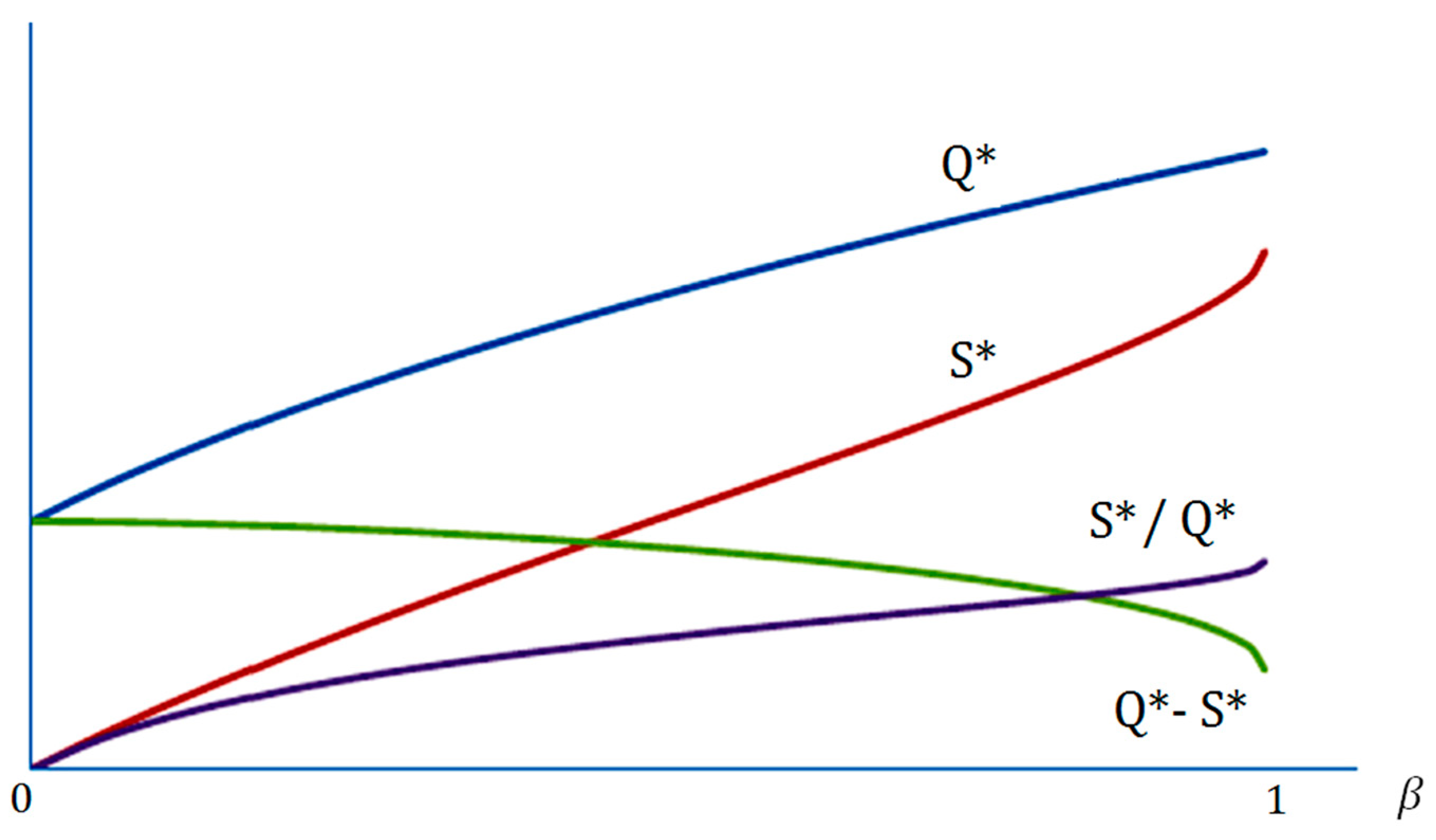
For the seventh issue, we recall the Proposition 5 of Sphicas [5]. We must point out that in Proposition 5 of Sphicas [5] “the lower T C 1 = 2 D K h { h / ( h + p ) } ” is a typo. The revised version should be T C 1 = 2 D K h { p / ( h + p ) } .
Next, we begin to discuss the intersection of Q S and S in Figure 1. We recall
S = 2 D K / h r ( 1 + r β 1 β ) / ( 1 + r ) ,
and
Q S = 2 D K / h ( 1 + r β + r 1 β ) / ( 1 + r ) .
We cite the following paragraphs from Sphicas [5]; “Another comment on the graph: It is drawn showing the two curves, Q S and S , intersecting each other. This happens if and only if the value of r is 1 . When r is less than 1, S is always below Q S . The point of intersection of Q S and S occurs when β = ( 3 r 1 ) / r ( 1 + r ) , provided r 1 .”
We will divide this problem into three cases: Case (a) 0 < r < 1 , Case (b) r = 1 , and Case (c) r > 1 .
For Case (a), with 0 < r < 1 , we derive that
1 + β r + r 1 β > r ( 1 + β r 1 β )
such that S is below Q S as claimed by Sphicas [5].
For Case (b), with r = 1 , we find that Q S = S if and only if 1 β = 0 , that is β = 1 . In Sphicas [5], he claimed that β ( 0 , 1 ) . In our previous discussion of the fourth issue, for Proposition 1 of Sphicas [5], we already revised the domain of β , from 0 < β < 1 to 0 β < 1 . Hence, 1 is not in the domain of β . We conclude then that r = 1 ; there is no intersection between Q S and S .
For Case (c), with r > 1 , we compute the intersection between Q S and S , to imply that
1 + β r + r 1 β = r ( 1 + β r 1 β ) .
We rewrite Equation (55) as
( r 1 ) 1 + β r = ( 1 + r ) 1 β ,
to square on both sides to yield
( r 1 ) 2 + r ( r 1 ) 2 β = ( 1 + r ) 2 ( 1 + r ) 2 β ,
such that we obtain that when r > 1 , the intersection satisfies
β = 4 r r 3 r 2 + 3 r + 1 .
Therefore, our finding of Equation (58) is a revision for the questionable assertion of Sphicas [5] of β = ( 3 r 1 ) / r ( 1 + r ) , provided r > 1 . We summarize our results in the next Theorem.
Theorem 2.
When r > 1 , the intersection of Q S and S occurs at β = 4 r r 3 r 2 + 3 r + 1 .
For completeness, the assertion of Sphicas [5], “this happens if and only if the value of r is 1 ”, should be revised from r 1 to r > 1 .
For the eighth issue, we recall the following assertion from Comment 1 of Section 4 of Sphicas [5]. We cite “Comment 1: The modified EOQ formula (4) (Equation (16) in this paper) can be viewed as a generalization of the two classical EOQ models. Mathematically, one could consider E O Q β as a combination of the two basic models, with β taking the role of a binary variable β = 0 or β = 1 and producing E O Q 0 or E O Q 1 , respectively.”
We must point out that in Proposition 1 of Sphicas [5], he mentioned that 0 < β < 1 . In our fourth issue, we improve the domain of β as 0 β < 1 . Hence, using β = 1 violates his definition of β .
The corrected expression should be improved as follows:
If we take the limit as β 1 , then E O Q β E O Q 1 .
For the ninth issue, we cite the following from Sphicas [5]; “The other values, S , Q S , and T C obviously also lie in-between the corresponding values of the two basic models, but no convenient linear combination form appears obtainable”, in Comment 1 of Section 4.
We recall that Sphicas [5] mentioned that
E O Q β 2 = ( 1 β ) E O Q 0 2 + β E O Q 1 2 .
Motivated by Equation (59), we will show that there is a δ such that
( Q 2 S 2 ) 2 = δ ( Q 0 S 0 ) 2 + ( 1 δ ) ( Q 1 S 1 ) 2 ,
to reveal that the assertion of Sphicas [5], in Comment 1 for Q S , as Q 2 S 2 lies in-between the corresponding values of Q 0 S 0 and Q 1 S 1 , contains questionable results.
We recall that
Q 0 S 0 = 2 D K h ,
Q 1 S 1 = Q 1 h h + p Q 1 = 1 1 + r Q 1 = 1 1 + r 2 D K h ,
and
Q 2 S 2 = ( 1 + β r + r 1 β 1 + r ) 2 D K h .
We plug Equations (61–63) into Equation (60) to derive that
( 1 + β r + r 1 β 1 + r ) 2 = δ + 1 δ 1 + r .
We simplify Equation (64) to yield that
δ = ( r 1 ) ( 1 β ) + 2 1 + β r 1 β 1 + r ,
to demonstrate that our goal of Equation (60) is derived.
For the tenth issue, we will show that there is a ε such that
( T C 2 ) 2 = ε ( T C 0 ) 2 + ( 1 ε ) ( T C 1 ) 2 ,
to reveal that the assertion of Sphicas [5], in Comment 1 for T C , as T C 2 lies in-between the corresponding values of T C 0 and T C 1 , contains questionable results.
We recall that
T C 0 = 2 h D K ,
T C 1 = 1 1 + r 2 h D K ,
and
T C 2 = ( 1 + β r + r 1 β 1 + r ) 2 h D K .
We plug Equations (67)–(69) into Equation (66) to derive that
( 1 + β r + r 1 β 1 + r ) 2 = ε + 1 ε 1 + r ,
which is identical to Equation (64), except the variable is changed from δ to ε . Hence, we obtain
ε = ( r 1 ) ( 1 β ) + 2 1 + β r 1 β 1 + r ,
to demonstrate that our goal of Equation (66) is derived. Therefore, the assertion of Sphicas [5], in Comment 1 with respect to T C contains questionable results.
For the eleventh issue, we cite the following from Comment 2 of Section 2; “Comment 2: A clear advantage of (4) [Equation (16) in this paper] over (1) [Equation (9) in this paper] is the absence of any negative terms under the square root. Although it is theoretically known that whenever (1) is valid it produces a real value, the reverse is not necessary true: (1) could produce a real value but not be valid, which was one of the points that were made in the earlier work cited here. In the new form (4) [Equation (16) in this paper], that observation can be rephrased as follows. If a negative β is inappropriately substituted in (3) [to the best of our knowledge, (3) is a typo, Sphicas should have typed (4); (3) of Sphicas [5] is Equation (15), the definition of β = M a x ( 0 , 1 π 2 D 2 2 h D K ) ], it could be small enough to keep 1 + ( β h / p ) positive. That would produce a real value for the square root but it would be inappropriate and irrelevant”.
First, we point out that Equations (1) and (4) of Sphicas [5] correspond to Equations (9) and (16) in this paper.
We must mention that researchers cannot directly compare Equations (9) and (16) in this paper. We recall that Equation (16) is the solution of E O Q β , which is a combination of two cases: Case (A): D π 2 h D K and Case (B): D π < 2 h D K .
For Case (A), with 2 h D K π 2 D 2 ,
E O Q β = 2 D K h .
and for Case (B), with 2 h D K > π 2 D 2 ,
E O Q β = 2 D K ( h + p ) π 2 D 2 h p .
On the other hand, the result of Equation (9), Q = E O Q 2 = 2 D K ( h + p ) π 2 D 2 h p is only suitable for Case (B), which is identical to Equation (73).
The findings of Equations (9) and (16) are suitable for two different domains, such that to compare them is meaningless.
In Equation (73), there is a negative term “ π 2 D 2 ”. However, we can rewrite Equation (73) as follows:
E O Q β = ( 2 h D K π 2 D 2 ) + 2 p D K h p ,
to show that there is no negative term in Equation (74), as 2 h D K > π 2 D 2 .
Hence, Sphicas [5] is criticized because Equation (73) containing a negative term is a false statement.
Second, there are many negative numbers, denoted as δ , satisfying 1 + ( δ h / p ) > 0 . For example, we take δ = p / 2 h , then
1 + δ h p = 1 + ( p 2 h ) h p = 1 2 > 0 ,
to demonstrate that there are many negative values that can satisfy 1 + ( δ h / p ) > 0 .
However, E O Q β of Equation (16) is developed by Sphicas [5], under the restriction of β 0 . β < 0 violates the definition of Sphicas [5]. Hence, we cannot understand why Sphicas [5] wanted to discuss the results with respect to β < 0 .
The advantage of (4) over (1) (that is Equation (16) and (9), in this paper) as mentioned in Comment 2 of Section 2 in Sphicas [5] is a misunderstanding, which we will show by the following.
In Equation (9), the optimal ordering quantity is derived as
Q = E O Q 2 = 2 D K ( h + p ) π 2 D 2 h p ,
to guarantee E O Q 2 > 0 , then the restriction 2 D K ( h + p ) > π 2 D 2 appears.
We recall Equation (13), for the optimal backorder quantity,
S = h ( E O Q 2 ) π D h + p
, such that to guarantee S > 0 , E O Q 2 > π D / h .
From E O Q 2 > 0 to a stronger condition E O Q 2 > π D / h , the insufficient condition
2 D K ( h + p ) > π 2 D 2
is strengthened to the desired condition
2 D K h > π 2 D 2 .
Sphicas [5] did not discuss the conditions of E O Q 2 > 0 and S > 0 .
We may predict that Sphicas [5] tried to remind researchers that there are some order quantities that satisfy E O Q 2 > 0 (with β < 0 , in Equation (16)), but they cannot be accepted as an order quantity.
We consider the problem of checking 1 + r β > 0 , that is
1 + h p max { 0 , 1 π 2 D 2 2 h D K } > 0 .
We concentrate on the restriction of
1 + h p ( 1 π 2 D 2 2 h D K ) > 0 .
We rewrite Equation (79) as
h + p p > ( h p ) π 2 D 2 2 h D K ,
and then we simplify the inequality of Equation (80) as
2 D K ( h + p ) > π 2 D 2 ,
which is identical to our discussion of Equation (76) as we expect for E O Q 2 > 0 .
Based on our above derivation to check 1 + r β > 0 , we finally come to the restriction of Equation (76).
However, we must point out that the examination of 1 + r β > 0 is tedious. The easy approach is directly referred to as Equation (9), and then researchers directly derive the restriction of Equation (76).
From our above discussion, Sphicas [5] not only forgot to check S > 0 , but also paid attention to a complicated expression of Equation (16). To check the positivity of Equation (16) is tedious. On the other hand, to check E O Q 2 > 0 by Equation (9) is straightforward.
Hence, we point out that the statement of Sphicas [5], “it could be small enough to keep 1 + ( β h / p ) positive. That would produce a real value for the square root but it would be inappropriate and irrelevant” is misleading and useless.
For the twelfth issue, we cite Section 5, Special cases, “the usual special cases noted in the literature include extreme values, such as 0 or infinity for various parameters. Here p = is fine, producing the E O Q 0 as a special case of E O Q β = 2 D K / h 1 + β h / p . Also admissible is the case of p = 0 , the situation of backordering everything for ever.”
If we plug p = 0 into Equation (8) to yield that
T C 2 ( Q , S ) = D K Q + h ( Q S ) 2 2 Q + D S π Q ,
and then we take partial derivatives of Equation (81) and solve Q T C = 0 and S T C = 0 , we derive that
h Q 2 = 2 D K + h S 2 + 2 π D S ,
and
h Q = h S + π D .
Based on Equations (82) and (83), we consider
h 2 Q 2 = 2 D K h + h 2 S 2 + 2 π D S h ,
and
h 2 Q 2 = ( h S + π D ) 2 .
From Equations (84) and (85), we derive that
2 D K h = π 2 D 2 .
Consequently, we divide our solution procedure into two cases: (i) 2 D K h π 2 D 2 , and (ii) 2 D K h = π 2 D 2 .
For case (i), under the condition 2 D K h π 2 D 2 , the first partial derivative system does not have a solution and the optimal solution will occur on the two boundaries: S = 0 and Q = S .
For p = 0 and S = 0 , the inventory model reduces to
T C 2 ( Q , S = 0 ) = D K Q + h Q 2 .
For p = 0 and Q = S , the inventory model reduces to
T C 2 ( Q = S , S ) = D K Q + π D .
From Equation (87), it is the T C 0 with the minimum value 2 D K h . From Equation (88), the inferior value, π D , occurs at Q .
Based on the above discussion, we further divide case (i) into two sub-cases: case (i-1) 2 D K h < π 2 D 2 , and case (i-2) 2 D K h > π 2 D 2 .
For case (i-1), owing to 2 D K h < π D , the minimum value occurs at T C 0 .
For case (i-2), from 2 D K h > π D , we know that numbers exist, denoted as Q # , that satisfy
2 D K h > D K Q # + π D ,
to yield that T C 0 > T C ( Q # , S = Q # ) . For example, if we take
Q 1 # = 2 D K 2 D K h π D ,
then we derive that
2 D K h ( D K Q 1 # + π D ) = 1 2 ( 2 D K h π D ) > 0 ,
then T C ( Q 1 # , S = Q 1 # ) is smaller than T C 0 = 2 D K h .
Hence, the minimum value occurs along the boundary, S = Q . From the mathematical point of view, the inferior value is
lim Q T C 2 ( Q , S = Q ) = π D .
However, Q is not possible in the real world. Therefore, for a practical situation, the decision maker will take an ordering quantity that is as large as possible to decrease the total cost along the boundary, S = Q .
On the other hand, for case (ii), under the condition 2 D K h = π 2 D 2 , Equations (82) and (83) degenerate to Equation (83). Hence, we compute T C 2 ( Q , S ) , under the restriction of h Q = h S + π D . Then for the interior solution,
T C 2 ( Q , S ) = D K Q + h ( Q S ) 2 2 Q + D S π Q = D K Q + π 2 D 2 2 Q h + D S π Q = D K Q + 2 D K h 2 Q h + D S π Q = 2 D K Q + D S π Q = 2 D K h + π D S h Q h = π 2 D 2 + π D S h Q h = π D ( π D + h S ) Q h = π D ,
for any pair of Q and S , satisfying h Q = h S + π D .
On the two boundaries, from Equation (87), T C 2 ( Q , S = 0 ) = 2 D K h and from Equation (88), the inferior value of T C 2 ( Q = S , S ) = π D .
Hence, for case (ii) with 2 D K h = π 2 D 2 , the minimum value is π D , that is 2 D K h . We summarize our findings in the next theorem.
Theorem 3.
For T C 2 , with p = 0 , there are three different results:
For case (i-1), with 2 D K h < π 2 D 2 , then the minimum value T C 2 = T C 0 ;
For case (i-2), with 2 D K h > π 2 D 2 , then the inferior value is π D as S = Q and Q approaches infinity.
For case (ii), with 2 D K h = π 2 D 2 , then the minimum value is π D = 2 D K h that is attained for any pair of Q and S , satisfying h Q = h S + π D .
Therefore, when p = 0 , only for case (i-2), the assertion of Sphicas [5] to backlog everything is true. On the other hand, for case (i-1), there is no shortage and then no backorders. Moreover, for case (ii), with the beginning inventory level, Q S = π D / h , and any backorder quantity S , will attain the minimum value π D .
Consequently, when p = 0 , we show that the intuitive assertion of Sphicas [5] to backlog everything is invalid.

5. Direction for Future Research

We notice that Sphicas [2] proposed his partition result before deriving the interior minimum solution. Moreover, in Sphicas [5], he did not provide a detailed explanation on how he partitioned the problem into two cases. Thus, practitioners might rely on the certain knowledge of final results in advance to apply Sphicas’ [2] solution, which is not realistic.
We can claim that, in the future, we will provide an enhanced solution procedure to derive and compare local minimums with reasonable classifications. After the optimal interior solution is obtained, several piecewise partitions will be synthesized to derive the compact partition as proposed in Sphicas [2], which will be an interesting research topic for future researchers.

Funding

This research received no external funding.

Conflicts of Interest

The author declares no conflict of interest.

References

  1. Johnson, L.A.; Montgomery, D.C. Operations Research in Production Planning, Scheduling, and Inventory Control; Wiley: New York, NY, USA, 1974. [Google Scholar]
  2. Sphicas, G.P. EOQ and EPQ with linear and fixed backorder costs: Two cases identified and models analyzed without calculus. Int. J. Prod. Econ. 2006, 100, 59–64. [Google Scholar] [CrossRef]
  3. Cárdenas-Barrón, L.E. The derivation of EOQ/EPQ inventory models with two backorders costs using analytic geometry and algebra. Appl. Math. Model. 2011, 35, 2394–2407. [Google Scholar] [CrossRef] [Green Version]
  4. Chung, K.; Cárdenas-Barrón, L.E. The complete solution procedure for the EOQ and EPQ inventory models with linear and fixed backorder costs. Math. Comput. Model. 2012, 55, 2151–2156. [Google Scholar] [CrossRef]
  5. Sphicas, G.P. Generalized EOQ formula using a new parameter: Coefficient of backorder attractiveness. Int. J. Prod. Econ. 2014, 155, 143–147. [Google Scholar] [CrossRef]
  6. Lin, S.S.C. Note on “The derivation of EOQ/EPQ inventory models with two backorders costs using analytic geometry and algebra”. Appl. Math. Model. 2019, 73, 378–386. [Google Scholar] [CrossRef]
  7. Grubbström, R.W. Material Requirements Planning and Manufacturing Resource Planning. In International Encyclopedia of Business and Management; Routledge: London, UK, 1996. [Google Scholar]
  8. Grubbström, R.W.; Erdem, A. The EOQ with backlogging derived without derivatives. Int. J. Prod. Econ. 1999, 59, 529–530. [Google Scholar] [CrossRef]
  9. Cárdenas-Barrón, L.E. The economic production quantity (EPQ) with shortage derived algebraically. Int. J. Prod. Econ. 2001, 70, 289–292. [Google Scholar] [CrossRef]
  10. Chang, H.C. A note on the EPQ model with shortages and variable lead time. Int. J. Inf. Manag. Sci. 2004, 15, 61–67. [Google Scholar]
  11. Sarker, B.R.; Coates, E.R. Manufacturing setup cost reduction under variable lead time and finite opportunities for investment. Int. J. Prod. Econ. 1997, 49, 237–247. [Google Scholar] [CrossRef]
  12. Ronald, R.; Yang, G.K.; Chu, P. Technical note: The EOQ and EPQ models with shortage derived without derivatives. Int. J. Prod. Econ. 2004, 92, 197–200. [Google Scholar] [CrossRef]
  13. Chang, S.K.J.; Chuang, J.P.C.; Chen, H.J. Short comments on technical note-The EOQ and EPQ models with shortages derived without derivatives. Int. J. Prod. Econ. 2005, 97, 241–243. [Google Scholar] [CrossRef]
  14. Lan, C.H.; Yu, Y.C.; Lin, R.H.J.; Tung, C.T.; Yen, C.P.; Deng, P.S. A note on the improved algebraic method for the EPQ model with stochastic lead time. Int. J. Inf. Manag. Sci. 2007, 18, 91–96. [Google Scholar]
  15. Luo, X.R.; Chou, C.S. Technical note: Solving inventory models by algebraic method. Int. J. Prod. Econ. 2018, 200, 130–133. [Google Scholar] [CrossRef]
  16. Lau, C.; Chou, E.; Dementia, J. Criterion to ensure uniqueness for minimum solution by algebraic method for inventory model. Int. J. Eng. Appl. Sci. 2016, 3, 71–73. [Google Scholar]
  17. Chiu, C.; Li, Y.; Julian, P. Improvement for criterion for minimum solution of inventory model with algebraic approach. IOSR J. Bus. Manag. 2017, 19, 63–78. [Google Scholar] [CrossRef]
  18. Sarkar, B. A production-inventory model with probabilistic deterioration in two-echelon supply chain management. Appl. Math. Model. 2013, 37, 3138–3151. [Google Scholar] [CrossRef]
  19. Noh, J.S.; Kim, J.S.; Sarkar, B. Stochastic joint replenishment problem with quantity discounts and minimum order constraints. Oper. Res. 2019, 19, 151–178. [Google Scholar] [CrossRef]
  20. Sarkar, B. Mathematical and analytical approach for the management of defective items in a multi-stage production system. J. Clean. Prod. 2019, 218, 896–919. [Google Scholar] [CrossRef]
  21. Sarkar, B.; Guchhait, R.; Sarkar, M.; Cárdenas-Barrón, L.E. How does an industry manage the optimum cash flow within a smart production system with the carbon footprint and carbon emission under logistics framework? Int. J. Prod. Econ. 2019, 213, 243–257. [Google Scholar] [CrossRef]
Figure 1.   Q = 2 K D / h 1 + β r   ,   S = 2 K D / h   r ( 1 + β r 1 β ) / ( 1 + r ) ,   S / Q = ( r / ( 1 + r ) ) ( 1 ( 1 β ) / ( 1 + β r )   ,   Q   S = 2 K D / h   ( 1 + β r + r 1 β ) / ( 1 + r ) Reproduction of Figure 1 of Sphicas [5].
Symmetry 11 00931 g001

