Article

Fake Bitrate Detection of HEVC Videos Based on Prediction Process

1
School of Electronic and Information Engineering, Beijing Jiaotong University, Beijing 100044, China
2
Guangdong Provincial Key Laboratory of Information Security Technology, Guangzhou 510000, China
3
School of Information Engineering, Beijing Institute of Graphic Communication, Beijing 100029, China
*
Author to whom correspondence should be addressed.
Symmetry 2019, 11(7), 918; https://doi.org/10.3390/sym11070918
Submission received: 29 June 2019 / Revised: 10 July 2019 / Accepted: 11 July 2019 / Published: 15 July 2019

Abstract

:
In order to defraud click-through rate, some merchants recompress the low-bitrate video to a high-bitrate one without improving the video quality. This behavior deceives viewers and wastes network resources. Therefore, a stable algorithm that detects fake bitrate videos is urgently needed. High-Efficiency Video Coding (HEVC) is a worldwide popular video coding standard. Hence, in this paper, a robust algorithm is proposed to detect HEVC fake bitrate videos. Firstly, five effective feature sets are extracted from the prediction process of HEVC, including Coding Unit of I-picture/P-picture partitioning modes, Prediction Unit of I-picture/P-picture partitioning modes, Intra Prediction Modes of I-picture. Secondly, feature concatenation is adopted to enhance the expressiveness and improve the effectiveness of the features. Finally, five single feature sets and three concatenate feature sets are separately sent to the support vector machine for modeling and testing. The performance of the proposed algorithm is compared with state-of-the-art algorithms on HEVC videos of various resolutions and fake bitrates. The results show that the proposed algorithm can not only can better detect HEVC fake bitrate videos, but also has strong robustness against frame deletion, copy-paste, and shifted Group of Picture structure attacks.

Graphical Abstract

1. Introduction

Digital video has become an indispensable part of our daily lives nowadays. According to the statistics, about 65,000 videos are uploaded to YOUTUBE every day [1]. However, falsified videos have been exposed to sneak in [2], which will cause serious moral, ethical, and legal problems. Therefore, it is essential to verify the authenticity of videos before they can be trusted. One of the video tampering methods is to up-convert the bitrate of a video without introducing any additional information about the video content. However, this operation does not improve the quality of the video, so we call this claimed high bitrate ‘fake bitrate’. The abused fake bitrate videos will not only mislead the viewers, but also lead to a big waste of storage space. Hence, it is necessary to propose an effective algorithm to detect fake bitrate videos.
In the process of making a fake bitrate video, the encoded video is decompressed before upconverting the bitrate and then recompressed after that. The re-encoding process may be different from that in the original video, in terms of video coding format and/or video coding parameters. Hence, the fake bitrate video is compressed twice at least. Therefore, detecting whether the video has been recompressed is a key step in detecting fake bitrate video. However, very limited work has been reported on detecting High-Efficiency Video Coding (HEVC) recompressed videos. In summary, the recompression detection methods can be divided into two categories: transformation-process-based method and prediction-process-based method. Discrete Cosine Transform (DCT) is adopted in the transformation process by most video codecs, thus it is logical to detect double compression by using DCT coefficients. References [3,4] detected double compression in MPEG (Moving Picture Experts Group) videos based on first digit distribution of DCT coefficients. Markov features calculated from the quantized DCT coefficients were used for double MPEG-4 compression detection [5]. After HEVC standard was published, Huang et al. [6,7,8] extracted the statistical characteristics such as Markov and co-occurrence matrix of DCT coefficients to detect recompressed HEVC videos. By analyzing the effects of Quantization Parameters (QP) on the distributions of DCT coefficients and TU size, Li et al. [9] proposed a method to detect HEVC video double compression with different QPs.
For prediction-process-based methods, Chen et al. [10] extracted the statistical feature from macroblock mode (MBM), which consisted of macroblock types and motion vectors in P-picture to detect double MPEG compression with the same QPs. Jiang et al. [11] concatenated the statistical features of rounding and truncation errors extracted from the intra-coding process and the macroblock-mode based features obtained from the inter-coding process to detect double recompressed MPEG and H.264 videos with the same coding parameters. By analyzing the characteristics of intra-coded macroblock and skipped macroblock of recompressed videos, Variation of Prediction Footprint (VPF) features were extracted to detect MPEG-x and H.264 recompression in [12]. After that, reference [13] combined block-artifacts of P-pictures with VPF features to detect recompressed MPEG-4 and H.264 videos. Compared with previous coding standards, HEVC introduces some new techniques in the prediction process to increase coding efficiency, especially the quadtree structure. According to the characteristics of the HEVC prediction process, Costanzo and Barni [14] counted up the motion prediction modes of P-pictures and B-pictures to distinguish whether the HEVC video has undergone AVC (Advanced Video Coding) first, and Jia et al. [15] applied the number of Prediction Unit (PU) blocks with the size of 4 × 4 in I-pictures to detect double-compressed HEVC video with the same QPs. Sequence of Number of Prediction Unit of its Prediction Mode (SN-PUPM) was exploited to detect HEVC recompression with different Group of Picture (GOP) sizes in [16]. Horizontal co-occurrence matrixes of DCT coefficients and the horizontal co-occurrence of PU partitioning modes in I-picture were combined in [17] to detect double HEVC compression.
To wrap up the previous HEVC recompression detection algorithms, most of them [6,7,8,9,15] were under the same or different QPs. Solutions to detect HEVC recompression with fake bitrate are rarely reported. Inspired by this, we presented an algorithm for detecting recompressed HEVC videos with fake bitrates [18]. Our previous work [18] only focused on the PU partitioning modes of the first P-picture in each GOP, and used the histogram of 25 PU partitioning modes of P-picture as the classification feature. Reference [18] confirmed that the HEVC recompression does affect the P-PU partitioning modes, while it did not comprehensively analyze other prediction variables in HEVC prediction process. However, there are six prediction variables generated in HEVC prediction process: Coding Unit of I-picture (I-CU) partitioning modes, PU of I-picture (I-PU) partitioning modes, Intra Prediction Modes (IPM) of I-picture (I-IPM), CU of P-picture (P-CU) partitioning modes, PU of P-picture (P-PU) partitioning modes, and IPM of P-picture (P-IPM). Therefore, in this paper, we will comprehensively analyze the relevant prediction variables generated in the prediction process to explore the correlation and independence among all the prediction variables. Overall, we present an algorithm to detect recompressed HEVC videos with fake bitrate by classification features extracted from prediction process. Firstly, we extract five single features, and sent them to Support Vector Mmachine (SVM) to verify their effectiveness. In order to enhance the expressiveness of the classification feature, single features are fused in three ways. Finally, three concatenation features are separately sent to SVM to distinguish recompressed HEVC videos with fake bitrate from single-compressed HEVC videos.
The main contributions of this paper are as follows. Firstly, we propose an efficient method to identify recompressed HEVC videos with fake bitrate, and its classification accuracy is much higher than the previous algorithms. Secondly, it is the first time, to the best of our knowledge, to comprehensively extract multiple effective prediction features from HEVC prediction process. Thirdly, the robustness of the proposed method is considered, and experimental results show that it has strong robustness against frame deletion, copy-paste, and shifted GOP structure attacks.
The rest of the paper is organized as follows. Section 2 briefly reviews the prediction process in HEVC and continued with the analysis of several effective prediction features under different fake bitrates in Section 3. Experimental results are shown in Section 4 and Section 5 concludes the paper.

2. Basics of Prediction Process in HEVC

In 2013, the HEVC standard was jointly ratified and published by ITU-T and ISO/IEC [19,20]. The video coding layer of HEVC employs the same hybrid approach (inter/intra prediction and 2-D transform coding) used in all video compression standards since H.261 [21]. The coding framework of HEVC is shown in Figure 1. It mainly includes bitrate control module, transformation and quantization module, prediction module, entropy coding module, and reconstruction module. It can be seen that the prediction module is a very important part of the coding process, and it is closely related to each module.
Prediction coding in HEVC uses the spatial and temporal correlation of the image signal to predict the current encoding pixel with its reconstructed pixel. There are two kinds of video signal prediction methods in HEVC: intra prediction and inter prediction. We use Figure 2 to describe the HEVC prediction process visually. In the prediction process of HEVC, each picture firstly performs CU and PU partitioning in a quadtree structure, and then selects the optimal IPM in each PU. The HEVC standard stipulates that I-picture only can opt intra prediction, while P-picture can adopt either intra or inter prediction.
Using the quadtree partitioning method, the coding tree unit (CTU) is divided into CUs and then the PU partitioning modes in each CU block are determined. A 64 × 64 luma of CTU can be split into multiple CUs with size from 8 × 8 to 64 × 64 (Figure 3a). The partitioning can be described by a quadtree structure, as shown in (Figure 3b), where the numbers indicate the index of the CUs in Figure 3a. Regardless of whether it is intra prediction or inter prediction, there are only four types of CU partitioning mode. The index of each CU partitioning modes is shown in Table 1.
The PU partitioning modes in intra prediction and inter prediction are shown in Figure 4. A CU can be symmetrically divided into one or four prediction blocks (PBs) for intra prediction. While in inter prediction, a CU can be divided into symmetric or asymmetric PBs. There are 5 PU partitioning modes in intra prediction and 25 PU partitioning modes in inter prediction, and their indexes are listed in Table 2 and Table 3.
In the intra prediction process, the optimal IPM is selected in each PU. HEVC defined 35 IPM, which are DC mode, 33 angle modes, and planar mode, as shown in Figure 5. The increase of intra prediction angles makes intra prediction more accurate, thereby reducing the spatial redundancy of video more effectively.

3. Prediction Features in HEVC Videos

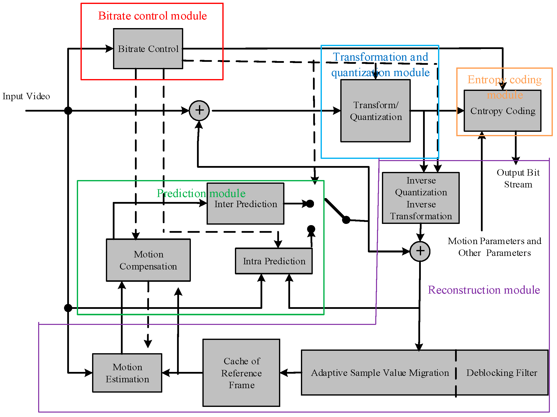
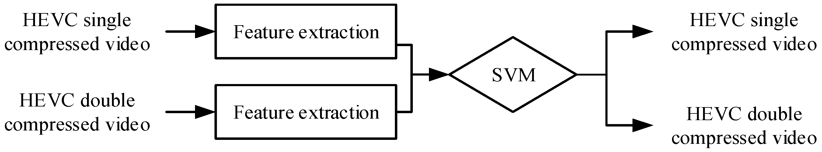
In this paper, we focus on proposing an effective algorithm to distinguish recompressed HEVC videos with fake bitrate from original videos. In the HEVC video recompression process, reconstruction error and quantization error are generated in the reconstruction process and quantization process, respectively. These two kinds of errors make the decoding video lose a part of content information, which further influence prediction variables: I-CU partitioning modes, I-PU partitioning modes, I-IPM, P-CU partitioning modes, P-PU partitioning modes, and P-IPM. The theoretical model and case study of the influence of irreversible coding errors on prediction variables will be described in detail in this section.

3.1. Theoretical Analysis and Modeling

For an original YUV (Luma and Chroma) sequence V ( V = { F n | n = 1 , 2 , , N } ), where F n denotes the nth frame and N is the total number of video frames. Given a bitrate r, the CU partitioning modes, PU partitioning modes, and IPM in I-picture and P-picture are successively determined. Let ρ ( ) represents the bit allocation process of rate control module, the amount of bits allocated to the nth frame can be written as b n ( r ) = ρ ( n ; V ; r ) . Please note that in this paper, a picture contains only one slice.
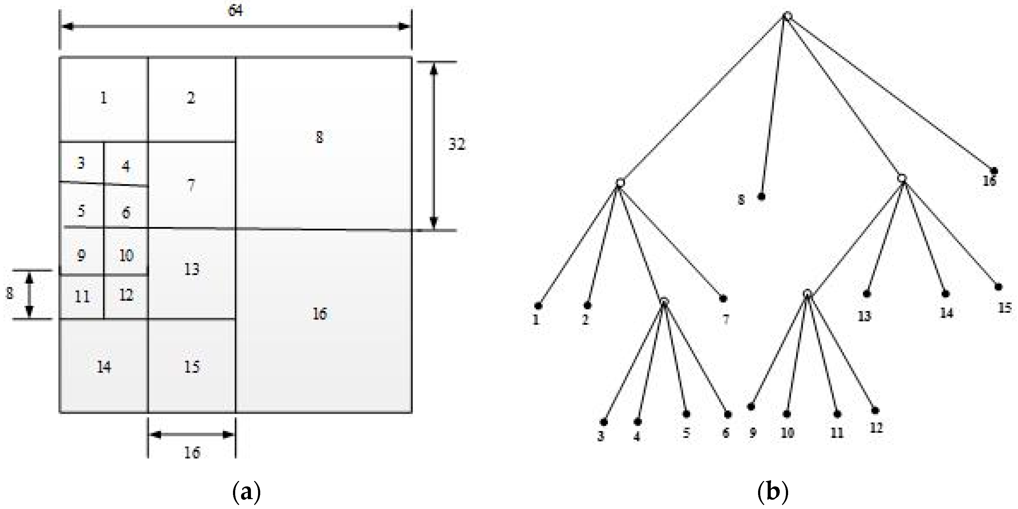
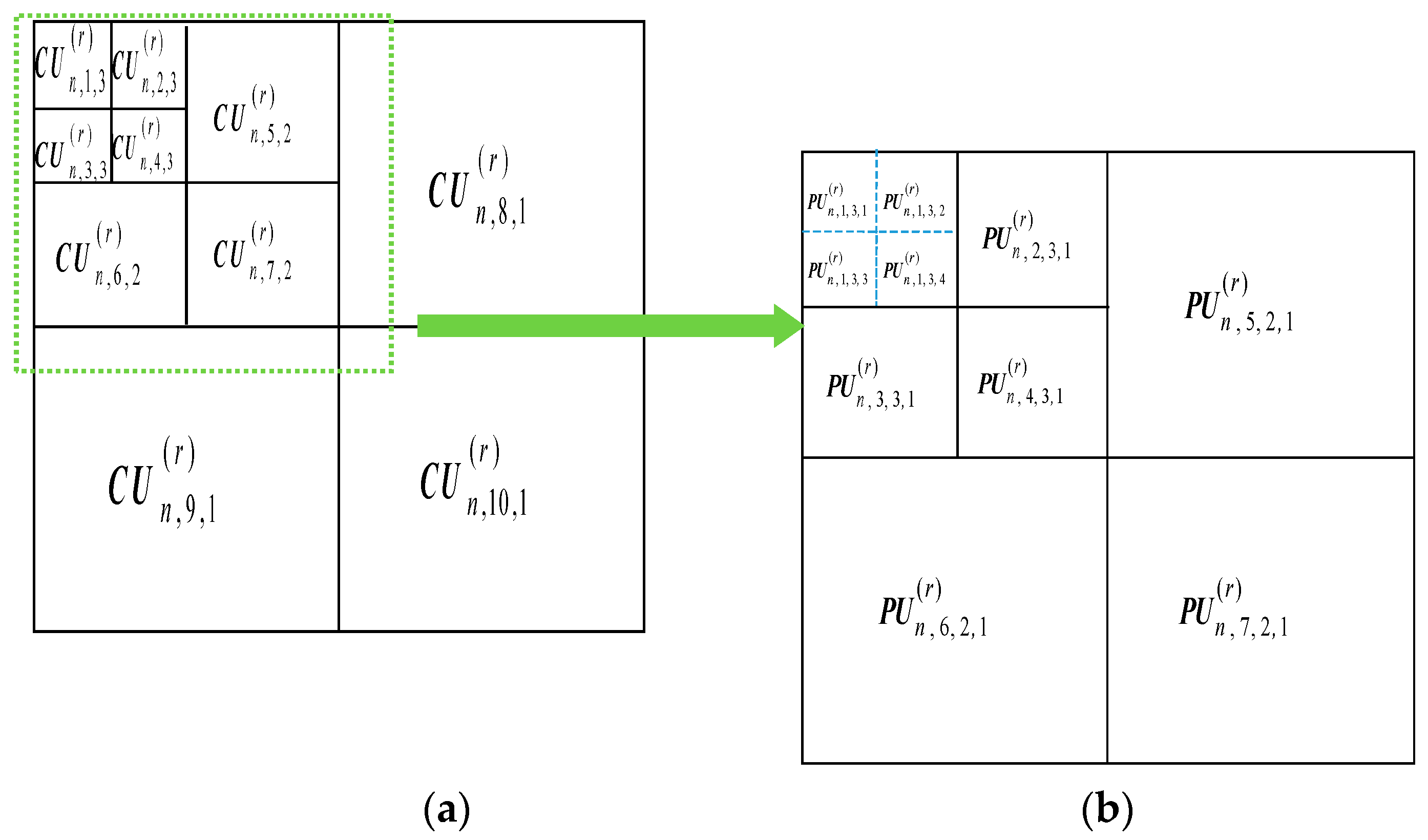
For intra prediction process π ( ) , it will select the optimal splitting of CTU into CUs, the optimal partitioning of CU into Pus, and the best IPM in PU to obtain the smallest rate-distortion value. Let k and K n represent the kth CU in the nth frame and the total number of CUs in the nth frame, respectively. The CU partitioning sequence with d partitioning depth in the nth frame can be denoted as C U intra ( r ) = { C U n , k , d ( r ) | k = 0 , 1 , 2 , , K n , d { 0 , 1 , 2 , 3 } } , where d = 0, 1, 2, 3 means the CU size is 64 × 64, 32 × 32, 16 × 16, 8 × 8, respectively. When the CU depth is 0 to 2, the PU partitioning mode is the same as the CU partitioning mode. When the CU depth is 3, the PU can either be 8 × 8 or 4 × 4. Therefore, the PU partitioning sequence in the nth frame can be denoted as P U intra ( r ) = { P U n , k , d , i ( r ) | i = { 1 , , I } , I = { 1 ; when   d = 0 , 1 , 2 1   or   4 ; when   d = 3 } , where i and I represent the ith PU in the kth CU and the total number of PUs contained in the kth CU, respectively. The IPM sequence in the ith PU can be represented as I P M intra ( r ) = { I P M n , k , d , i , j ( r ) | j { 1 , 2 , 3 , , 35 } } , where I P M n , k , d , i , j ( r ) denotes an IPM whose index is j of the ith PU in the kth CU whose depth is d in the nth frame.
In order to demonstrate the subscript more clearly, we draw a CTU with size of 64 × 64 in the nth frame as an example. The CU sequence of the CTU is shown in Figure 6a, the PU sequence of the 32 × 32 CU in the upper left corner of Figure 6a is shown in Figure 6b. The index of each CU is counted from up to down and from left to right.
The sequences of CU partitioning modes, PU partitioning modes, and IPMs in intra prediction process can be represented as Equation (1). We can see that CU partitioning modes, PU partitioning modes, and IPMs in intra prediction are mainly affected by the picture content and the bits allocated to the frame.
( I P M intra ( r ) , P U intra ( r ) , C U intra ( r ) ) = π ( F n ; b n ( r ) )
For inter prediction process f ( ) , the partition strategy is similar to intra prediction. The CU partitioning sequence with d depth in the nth frame can be represented as C U inter ( r ) = { C U n , k , d ( r ) | k = 0 , 1 , 2 , , K n , d { 0 , 1 , 2 , 3 } } 
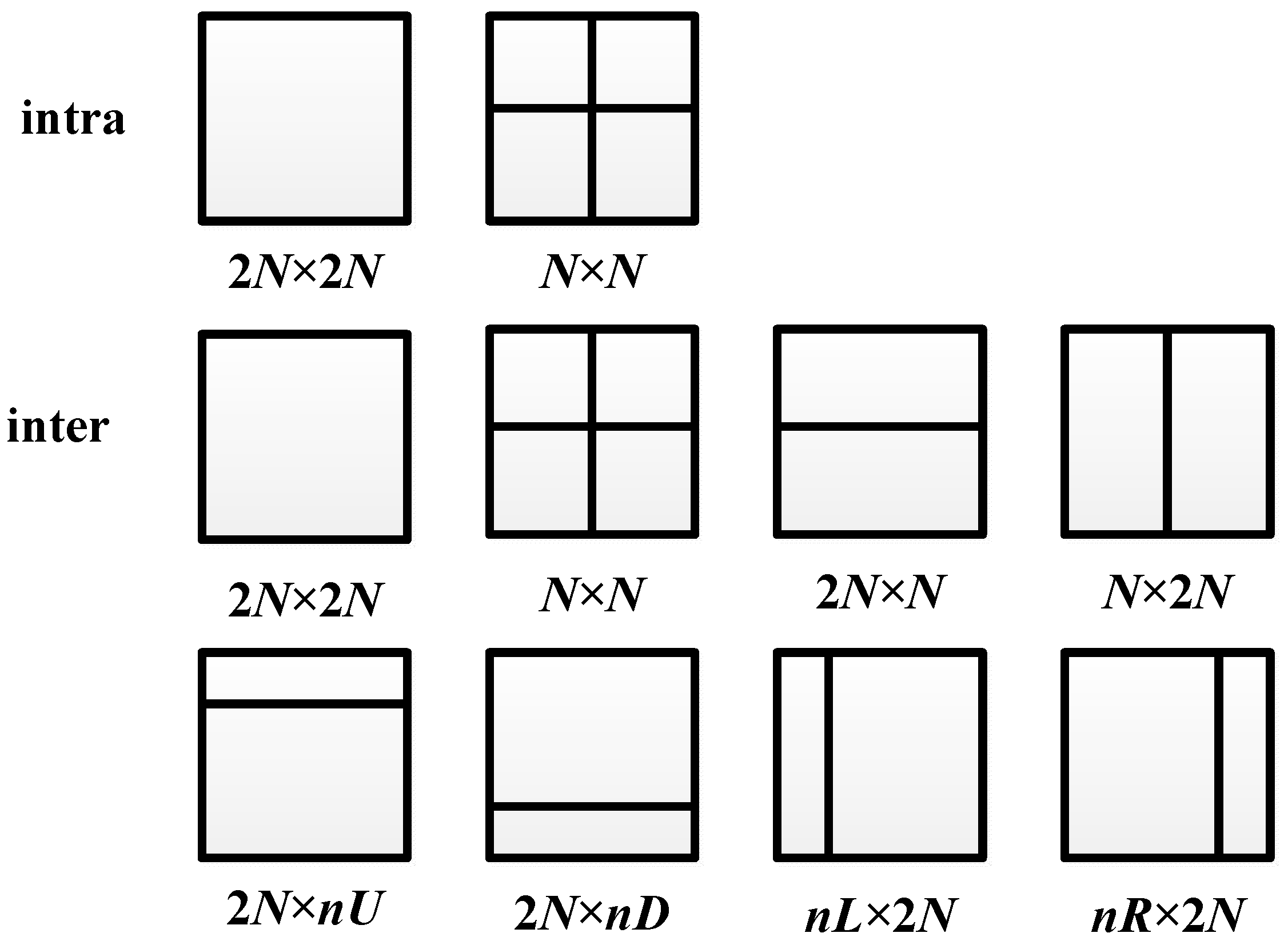
. Different from the case in intra prediction, apart from symmetric partitioning modes, inter prediction also has asymmetric PU partitioning modes, as shown in Figure 4. Therefore, the inter PU partitioning sequence in the nth frame can be represented as P U inter ( r ) = { P U n , k , d , i ( r ) | i = { 1 , , I } , I   = { 1 or 4 ;   when d = 3 1 or 2 ;   when d = 0 , 1 , 2 } , where i and I represent the ith PU in the kth CU and the total number of PUs contained in the kth CU, respectively. When the size of the kth CU is 64 × 64 or 32 × 32 or 16 × 16 (d = 0 or 1 or 2), the kth CU can be symmetric or asymmetric partitioned, so I = 1 or 2. When d = 3, it is the same as intra prediction. There is no IPM exist in inter prediction. Thus, the CU partitioning sequence and PU partitioning sequence in inter prediction process can be represented as Equation (2), where C n is the reference frame of F n . That is to say, the CU partitioning modes and PU partitioning modes in inter prediction are not only determined by the content of the picture and the bits allocated to the frame, but also by the content of the reference frame.
( P U inter ( r ) , C U inter ( r ) ) = f ( F n ; b n ( r ) ; C n )
We use the P-PU partitioning sequence as an example to describe the difference between HEVC recompressed video with fake bitrate and single-compressed video. As shown in Figure 2, P-picture can use either intra prediction or inter prediction. That is to say, P-PU partitioning sequence in a HEVC video denoted as P P U ( r ) is composed of PU partitioning sequence by adopting intra prediction and that by adopting inter prediction. Therefore, the P-PU partitioning sequence P P U ( r ) can be expressed as Equation (3).
P P U ( r ) = P U intra ( r ) P U inter ( r )
Assume that the first and second compression bitrates of the recompressed video are r 1 and r 2 ( r 1 r 2 for abbreviation), respectively. Here, we only consider the fake bitrate recompression situation, that is, the bitrate up-converting, so r 1 < r 2 . In the second compression, the amount of bits allocated to the nth P-frame can be written as Equation (4), where V ^ ( V ^ = { F ^ n | n = 1 , 2 , , N } represents the decoded YUV sequence, and F ^ n is the decompressed picture of F n . The P-PU partitioning sequence of HEVC recompressed video is P P U ( r 1 , r 2 ) .
b n ( r 1 , r 2 ) = ρ ( n ; V ^ ; r 2 )
P P U ( r 1 , r 2 ) = P U intra ( r 1 , r 2 ) P U inter ( r 1 , r 2 )
For HEVC single-compressed video with bitrate r 2 , b n ( r 2 ) is denoted as the amount of bits allocated to the nth P-picture, and P P U ( r 2 ) is the P-PU partitioning sequence of this single-compressed video. We can achieve
b n ( r 2 ) = ρ ( n ; V ; r 2 ) ,
P P U ( r 2 ) = P U intra ( r 2 ) P U inter ( r 2 ) .
Use D ( ) to represent the difference between P P U ( r 1 , r 2 ) and P P U ( r 2 ) . According to Equations (1)–(7), we can get the difference between the P-PU partitioning sequence of HEVC single-compressed videos and its corresponding recompressed videos with fake bitrate, as shown in Equation (8), where F ^ n and C ^ n are the decompressed version of F n and C n , respectively.
D ( P P U ( r 1 , r 2 ) , P P U ( r 2 ) ) = D ( ( P U intra ( r 1 , r 2 ) P U inter ( r 1 , r 2 ) ) , ( P U intra ( r 2 ) P U inter ( r 2 ) ) ) = D ( ( π ( F ^ n ; b n ( r 1 , r 2 ) ) f ( F ^ n ; b n ( r 1 , r 2 ) ; C ^ n ) ) ( π ( F n ; b n ( r 2 ) ) f ( F n ; b n ( r 2 ) ; C n ) ) ) = D ( ( π ( F ^ n ; ρ ( n ; { F ^ n | n = 1 , 2 , , N } ; r 2 ) ) f ( F ^ n ; ρ ( n ; { F ^ n | n = 1 , 2 , , N } ; r 2 ) ; C ^ n ) ) ( π ( F n ; ρ ( n ; { F n | n = 1 , 2 , , N } ; r 2 ) ) f ( F n ; ρ ( n ; { F n | n = 1 , 2 , , N } ; r 2 ) ; C n ) ) )
It can be concluded from Equation (8) that the main difference between P P U ( r 1 , r 2 ) and P P U ( r 2 ) comes from the contents of F n , F ^ n , C n , and C ^ n . The relation between F ^ n and F n can be derived as Equation (9), where E ( F n ) and E ( C n ) are the quantization error of F n and C n under the given quantization step Q p , respectively, [] means rounding operation. Therefore, we can get F ^ n F n = E ( F n ) E ( C n ) , which means the difference between F ^ n and F n is caused by quantization error and reconstruction error. Quantization error contains rounding error and truncation error in the quantization process. Reconstruction error is caused by reference frame in the reconstruction process. It means that the difference between P-PU partitioning sequence in HEVC double-compressed video with fake bitrate and single-compressed video is mainly caused by quantization error and reconstruction error.
F ^ n = IDCT ( [ DCT ( F n C n ) / Q p ] × Q p ) + C n IDCT ( [ DCT ( F n ) / Q p ] × Q p ) IDCT ( [ DCT ( C n ) / Q p ] × Q p ) + C n = F n + E ( F n ) E ( C n )
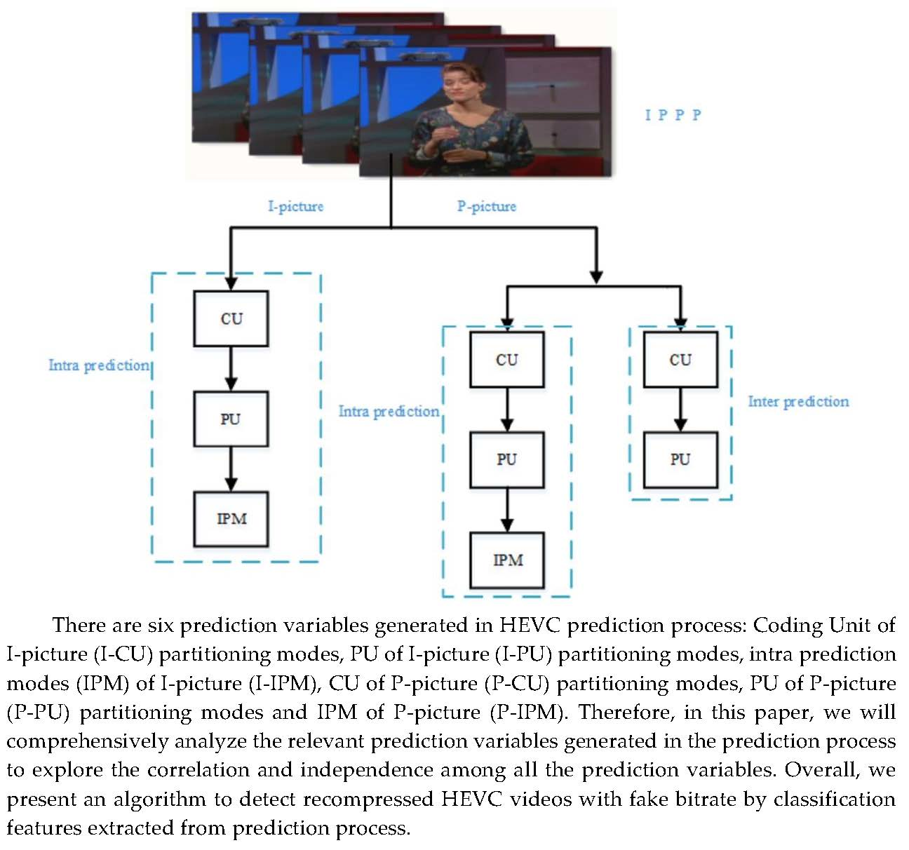
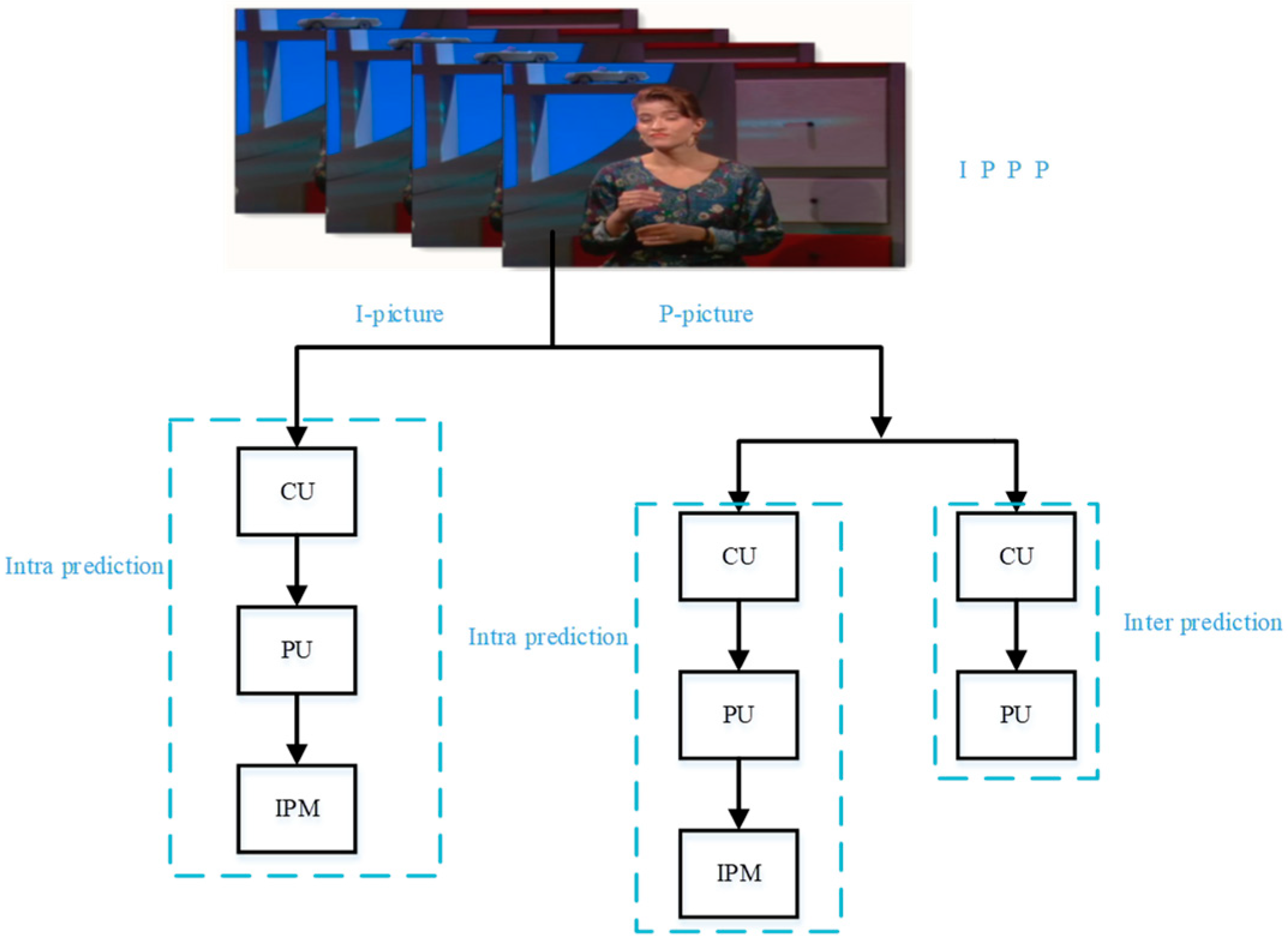
There are six kinds of prediction variables as illustrated in Figure 2. Similar as P-PU partitioning sequence P P U ( r ) , we can get other prediction sequences: I-CU partitioning sequence I C U ( r ) , I-PU partitioning sequence I P U ( r ) , I-IPM sequence I I P M ( r ) , P-CU partitioning sequence P C U ( r ) , P-IPM sequence P I P M ( r ) . And the difference between other prediction sequences of HEVC recompressed video and that of single-compressed video can be illustrated in Equations (10)–(13), respectively. Please note that the theoretical model of I I P M ( r ) and P I P M ( r ) are the same because IPM only appears in the intra prediction process.
D ( I C U ( r 1 , r 2 ) , I C U ( r 2 ) ) = D ( C U intra ( r 1 , r 2 ) , C U intra ( r 2 ) ) = D ( π ( F ^ n ; b n ( r 1 , r 2 ) ) , π ( F n ; b n ( r 2 ) ) ) = D ( π ( F ^ n ; ρ ( n ; { F ^ n | n = 1 , 2 , , N } ; r 2 ) ) , π ( F n ; ρ ( n ; { F n | n = 1 , 2 , , N } ; r 2 ) ) )
D ( P C U ( r 1 , r 2 ) , P C U ( r 2 ) ) = D ( ( C U intra ( r 1 , r 2 ) C U inter ( r 1 , r 2 ) ) , ( C U intra ( r 2 ) C U inter ( r 2 ) ) ) = D ( ( π ( F ^ n ; b n ( r 1 , r 2 ) ) f ( F ^ n ; b n ( r 1 , r 2 ) ; C ^ n ) ) , ( π ( F n ; b n ( r 2 ) ) f ( F n ; b n ( r 2 ) ; C n ) ) ) = D ( ( π ( F ^ n ; ρ ( n ; { F ^ n | n = 1 , 2 , , N } ; r 2 ) ) f ( F ^ n ; ρ ( n ; { F ^ n | n = 1 , 2 , , N } ; r 2 ) ; C ^ n ) ) , ( π ( F n ; ρ ( n ; { F n | n = 1 , 2 , , N } ; r 2 ) ) f ( F n ; ρ ( n ; { F n | n = 1 , 2 , , N } ; r 2 ) ; C n ) ) )
D ( I P U ( r 1 , r 2 ) , I P U ( r 2 ) ) = D ( P U intra ( r 1 , r 2 ) , P U intra ( r 2 ) ) = D ( π ( F ^ n ; b n ( r 1 , r 2 ) ) , π ( F n ; b n ( r 2 ) ) ) = D ( π ( F ^ n ; ρ ( n ; { F ^ n | n = 1 , 2 , , N } ; r 2 ) ) , π ( F n ; ρ ( n ; { F n | n = 1 , 2 , , N } ; r 2 ) ) )
D ( I I P M ( r 1 , r 2 ) , I I P M ( r 2 ) ) = D ( I P M intra ( r 1 , r 2 ) , I P M intra ( r 2 ) ) = D ( π ( F ^ n ; b n ( r 1 , r 2 ) ) , π ( F n ; b n ( r 2 ) ) ) = D ( π ( F ^ n ; ρ ( n ; { F ^ n | n = 1 , 2 , , N } ; r 2 ) ) , π ( F n ; ρ ( n ; { F n | n = 1 , 2 , , N } ; r 2 ) ) )
From Equations (10)–(13), we can conclude that the difference between the six prediction variable sequences in HEVC recompressed video and single-compressed video is mainly caused by irreversible quantization error and reconstruction error. Therefore, we consider that these six prediction variables can be used as classification features to distinguish HEVC recompression videos with fake bitrate and single ones.

3.2. Feature Analysis and Example Description

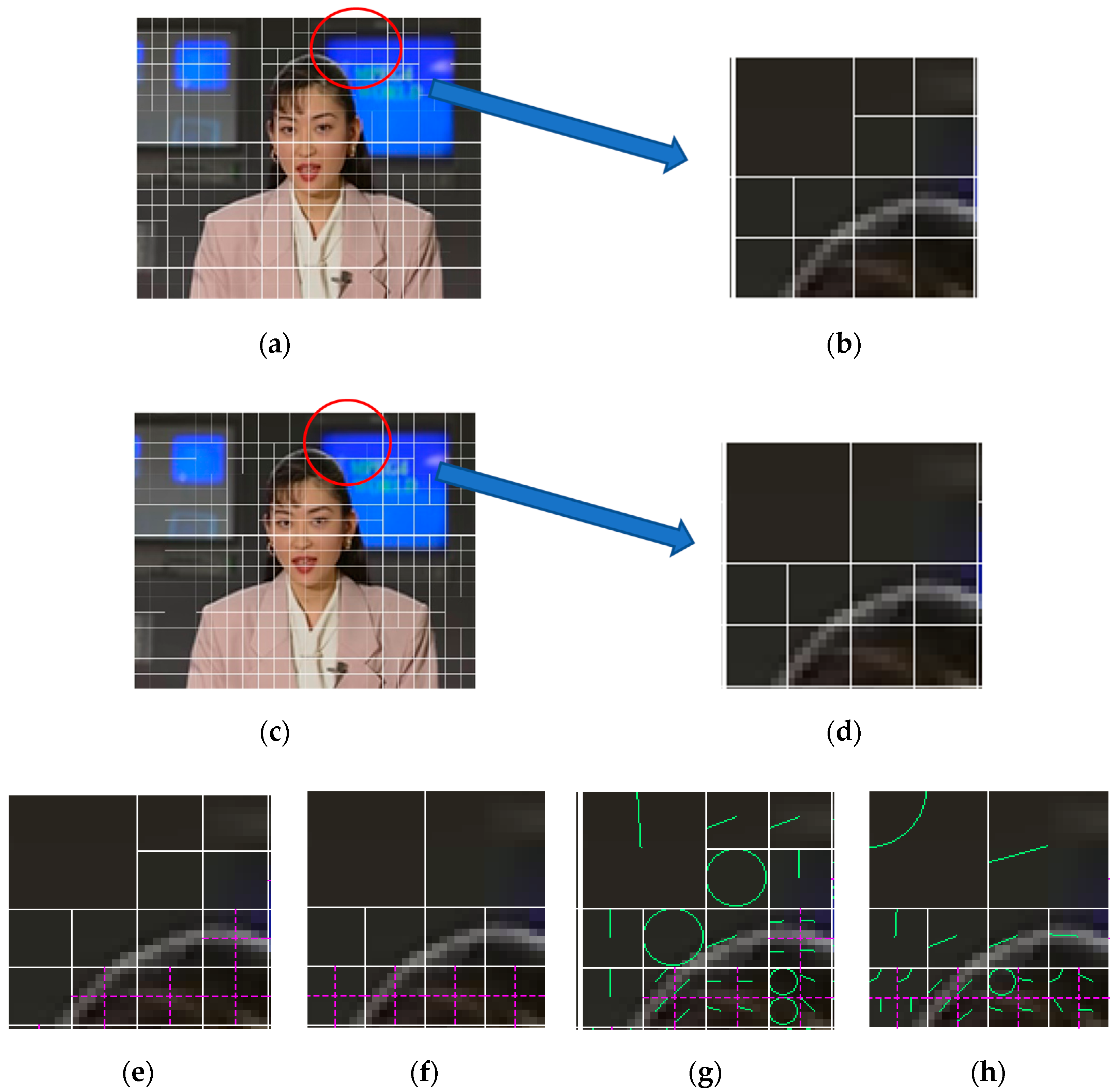
To illustrate the difference between prediction variables in fake bitrate recompressed video and single-compressed video, we will extract the CU partitioning modes, PU partitioning modes, and IPM of the same I-frame within the recompressed video with fake bitrate 100–400 Kbps and within the corresponding single-compressed video with bitrate 400 Kbps, as shown in Figure 7. The 16th picture (I-picture) with CU partitioning is extracted from the double-compressed video with fake bitrate as shown in Figure 7a, and the same frame of the single-compressed video is shown in Figure 7c. Taking the 32 × 32 block (shown in Figure 7b,d) surrounded by the red circle in the I-frame as an example for analysis. The block with PU partitioning modes in double- and single-compressed videos are shown in Figure 7e,f, respectively. Figure 7g,h exhibit the block with IPM in double- and single-compressed video, respectively. Observing Figure 7, it can be found that the three prediction variables (I-CU partitioning modes, I-PU partitioning modes, I-IPM) in the same I-picture of single-compressed video and double-compressed video with fake bitrate are quite different. Therefore, these three prediction variables of I-picture can be used as independent classification features for detecting fake bitrate recompression videos. In addition, even within the same I-CU partitioning block, the I-PU partitioning mode in single-compressed frame and recompressed frame is not necessarily the same, as is IPM, so these three prediction variables of I-picture are interdependent. As we can see, I-IPM is based on I-PU partitioning modes, and I-PU partitioning modes is based on I-CU partitioning modes, thus, the fusion method of concatenating these three single features can be used to enhance feature expression.
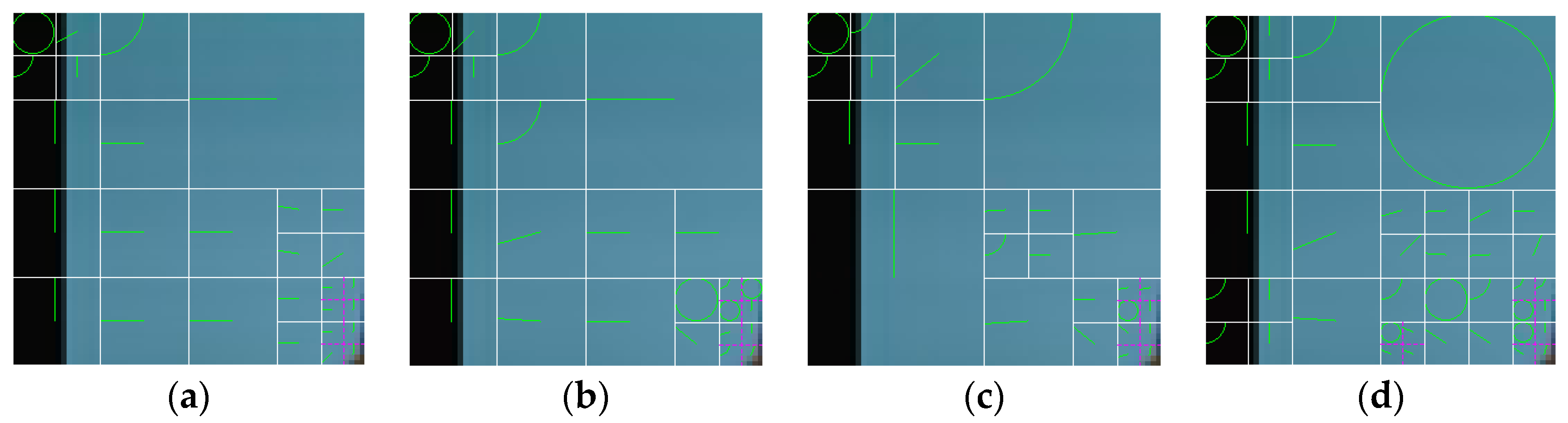
Four 64 × 64 blocks are extracted from the 7th I-picture in the “claire_qcif.yuv” with different bitrates, as shown in Figure 8. The white line indicates the CU partitioning, the purple line indicates the PU partitioning under the CU, and the green line indicates the IPM under the PU. Figure 8a is extracted from the single-compressed video with bitrate 400 Kbps, Figure 8b is extracted from the recompressed video with bitrate 300–400 Kbps, Figure 8c is extracted from the recompressed video with bitrate 200–400 Kbps, and Figure 8d is extracted from the recompressed video with bitrate 100–400 Kbps. Compared with the single-compressed video block (Figure 8a), the I-CU partitioning, I-PU partitioning, and I-IPM in the recompressed video blocks will change, the number of changes is shown in Table 4. Both visually and statistically, it can be seen that when the difference between the first bitrate and the second bitrate of the recompressed video becomes smaller, the difference between the prediction variables of I-picture in single-compressed video and double-compressed video will become smaller, the same as the prediction variables of P-picture.
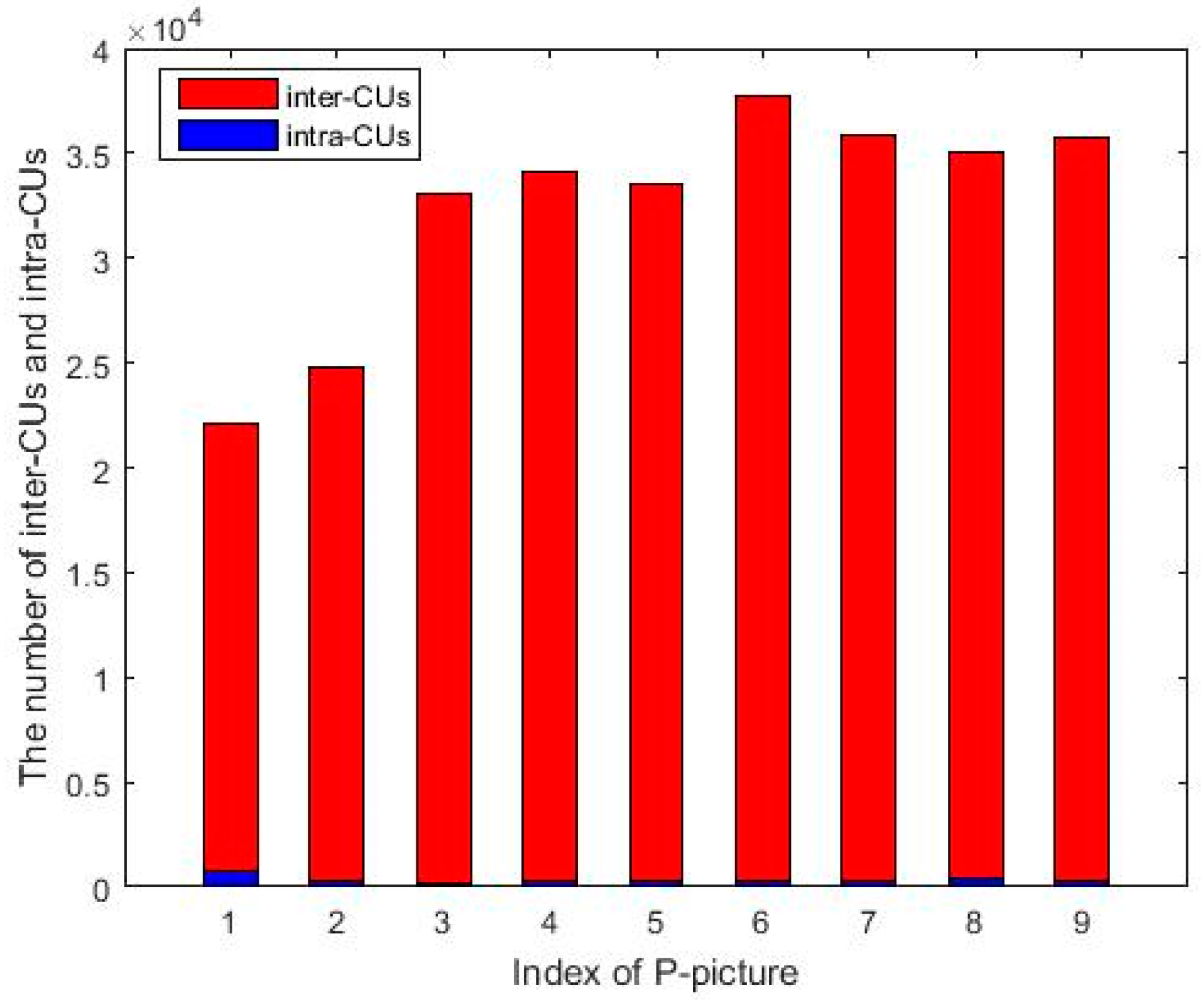
In P-picture, CU block traverses the various modes of inter prediction and intra prediction, and then selects the mode with the lowest rate distortion cost as the final optimal prediction mode. While the temporal redundancy in the video is more than the spatial redundancy, the efficiency of the general inter prediction is higher than that of the intra prediction. Therefore, most of the P-pictures select inter prediction instead of intra prediction. This phenomenon is indeed ubiquitous in HEVC videos, for example, randomly selecting 9 P-pictures from a HEVC single-compressed video. Then, separately counting the number of CU blocks which adopt intra prediction (abbreviated as “intra-CUs”) and the number of CU blocks which adopt inter prediction (abbreviated as “inter-CUs”) in each P-pictures, the statistical histogram is shown in Figure 9. The red bars represent the inter-CUs and blue bars represent the intra-CUs. It can be seen that intra-CUs only take a tiny percentage of the total CUs and they are much smaller than inter-CUs. Furthermore, there are 35 IPM choices for each PU block, which makes the number of each IPM mode too small in P-pictures to be used as a single classification feature. Therefore, we ignore the P-IPM and only adopt the other two prediction variables for P-pictures: P-CU partitioning modes and P-PU partitioning modes. Similarly, the CU partitioning modes and the PU partitioning modes of P-picture are mutually dependent.
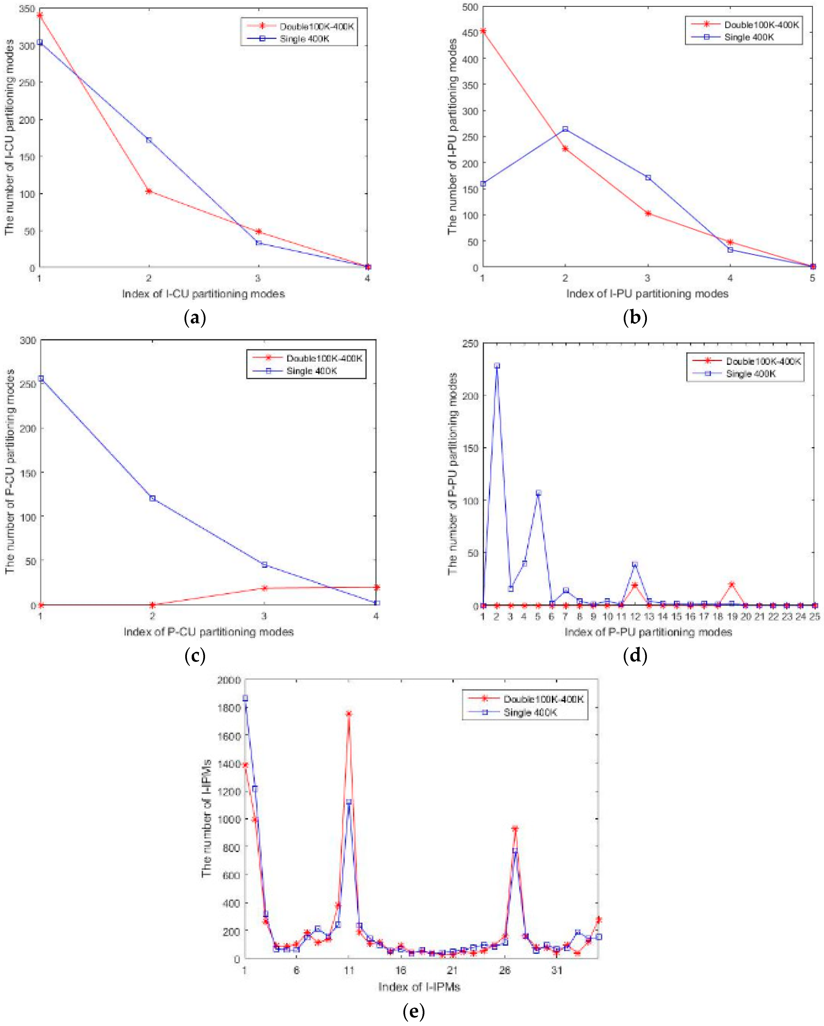
In the following, we will use a line chart to show the difference between the five prediction variables in the HEVC double-compressed video and the single-compressed video, as shown in Figure 10. The bitrate of the HEVC single-compressed video is 400 Kbps (blue lines) and the corresponding recompressed video with the first compression bitrate r 1 = 100   KbpS and the second compression bitrate r 2 = 400   KbpS (red lines). The abscissa indicates the index of the mode used in the prediction variable, and the ordinate indicates the total number of times the mode used in the prediction variable appears in the video. It is clearly that the difference between the red and blue lines in Figure 10a–d is obvious, which means the four prediction variables (I-CU partitioning modes, I-PU partitioning modes, P-CU partitioning modes, P-PU partitioning modes) can effectively distinguish HEVC single-and double-compressed videos. In 
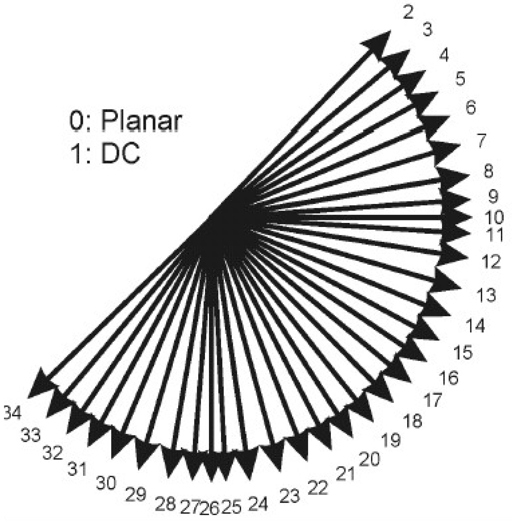
Figure 10e, we find that the number of I-IPM only differs greatly in the 1st, 2nd, 10th, 11th, 26th, and 27th intra prediction modes, and this phenomenon appears in most videos. Thus, we only use these six modes as the representatives of I-IPM.

3.3. The Proposed Target Features

From the above analysis, we know that the numbers of the five prediction variables are different between double-compressed videos with fake bitrate and single ones. In order to make the characteristics of the prediction variables more universal, we consider using the probability matrix of prediction variables as the classification features. The probability set can be expressed as Equations (14) and (15), where f i denotes the probability matrix of the ith prediction variable, where i = 1, 2, 3, 4, 5 represents 4-dimensional I-CU partitioning modes, 5-dimensional I-PU partitioning modes, 6-dimensional I-IPM, 4-dimensional P-CU partitioning modes, and 25-dimensional P-PU partitioning modes, respectively. M i represents the dimensions of each prediction variable, so M i = { 4 , 5 , 6 , 4 , 25 | i = 1 , 2 , 3 , 4 , 5 } . x i j represents the number of the jth mode of the ith prediction variable in a HEVC video. p i j represents the probability of the jth mode for ith prediction variable in the whole video. For example, for I-CU partitioning modes, i = 1, M 1 = 4, j = 1, 2, 3, 4. The number of each I-CU partition modes in the HEVC video are x 1 j , respectively, and their probabilities are expressed as p 1 j = x 1 j / j = 1 M 1 x 1 j , then, the probability matrix of I-CU partitioning modes is f 1 
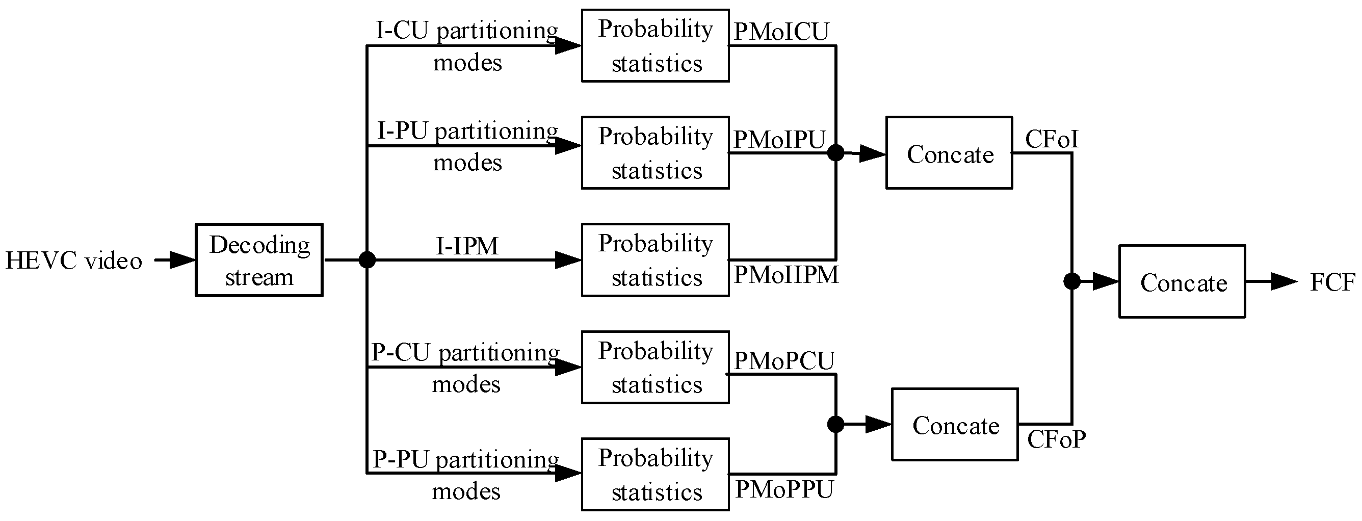
. The probability matrix of other prediction variables is similar to that of I-CU partitioning modes. Finally, we can get five single features: the probability matrix of I-CU partitioning modes (PMoICU) with dimensions of 4, the probability matrix of I-PU partitioning modes (PMoIPU) with dimensions of 5, the probability matrix of I-IPM (PMoIIPM) with dimensions of 6, the probability matrix of P-CU partitioning modes (PMoPCU) with dimensions of 4, and the probability matrix of P-PU partitioning modes (PMoPPU) with dimensions of 25.
F = { f i | i = 1 , 2 , , 5 }
f i = { p i j | p i j = x i j / j = 1 M i x i j , j = 1 , 2 , , M i }
According to Section 3.2, CU partitioning modes, PU partitioning modes, and IPM are interdependent, the feature fusion method can enhance the expressiveness of single features. Therefore, we concatenate these single features from three aspects, which are called Concatenation Feature of I-picture (CFoI), Concatenation Feature of P-picture (CFoP), and Full Concatenation Feature (FCF). CFoI with dimensions of 15 is made up of PMoICU, PMoIPU, and PMoIIPM; CFoP with dimensions of 29 is composed of PMoPCU and PMoPPU, while FCF with dimensions of 44 is concatenated by all single features.

3.4. The Flow of the Proposed Algorithm

The flow of the proposed algorithm is shown in Figure 11. The classification feature is extracted from the HEVC video, and then the feature is sent to the SVM classifier for model training and testing to determine whether the video is single-compressed video or double-compressed video with fake bitrate.
The process of feature extraction of the proposed algorithm is shown in Figure 12. Five prediction variables are extracted from the decoding stream of HEVC video. Based on the whole HEVC video, probabilistic statistics are performed on the five prediction variables to obtain five single features, respectively. Then, PMoICU, PMoIPU, and PMoIIPM are concatenated into CFoI, PMoPCU and PMoPPU are concatenated into CFoP, and finally, CFoI and CFoP are concatenated into the final classification feature FCF of the proposed algorithm.

4. Experimental Results

In this section, the performance of the proposed method is investigated on HEVC single- and double-compressed videos in QCIF (Quarter Common Interchange Format), CIF (Common Interchange Format), 720p, and 1080p video sets. The resolution of these four video sets are 176 × 144, 352 × 288, 1280 × 720, and 1920 × 1080, respectively. Each YUV sequence [22] is cut into several non-overlapping subsequences with 100 frames. Finally, we can obtain 36 QCIF videos, 43 CIF videos, 36 720p videos, and 32 1080p videos with YUV420P pixel format. The GOP size is set to 4 with the IPPP structure both in single- and double-compressed videos, and the rate control is enabled in the encoding process. Because this paper is for detecting recompressed video with fake bitrate, that is, the second bitrate of the recompressed video in our video sets is greater than the first bitrate (bitrate up-converting case), regardless of the cases of bitrate dropping or equal. To guarantee the quality of videos, for double compression video, the first compression bitrates is selected from r 1 = {100 K, 200 K, 300 K} (bps) for QCIF and CIF video sets, r 1 = {10 M, 20 M, 30 M} (bps) for 720p video set and r 1 = {10 M, 30 M, 50 M} (bps) for 1080p video set, the second compression bitrate is selected from r 2 = {200 K, 300 K, 400 K} (bps) for QCIF and CIF video sets, r 2 = {20 M, 30 M, 40 M} (bps) for 720p video set, and r 2 = {30 M, 50 M, 70 M} (bps) for 1080p video set. The bitrate of the corresponding single-compressed video is r 2 .
The accuracy rate (AR) is used as the criterion and calculated by AR = (TPR + TNR)/2, where TPR and TNR mean true positive rate and true negative rate, respectively. For the LIBSVM [23] classifier, PolySVC kernel is selected and the optimal parameters of the classifier are obtained by a round-robin algorithm. The entire classification procedure is repeated for 20 times and the average AR is considered as the final classification accuracy. The ratio of videos in training and testing sets is set to be 5:1 for each video set, the videos are randomly assigned to training or testing set, and each training set and test set is non-overlapping. Each single prediction feature will be tested separately to verify its validity, and then the concatenation features CFoI, CFoP, and FCF will be tested immediately. The robustness of the proposed method against frame-deletion, copy-paste, and shifted GOP structure attacks will be also discussed.

4.1. Single Features of I-Picture

From Section 3, we know that single features related to I-pictures are PMoICU, PMoIPU, and PMoIIPM, and their dimensions are 4, 5, and 6, respectively. In this section, their classification accuracies on four video sets are tested and shown in Table 5, Table 6 and Table 7. As we can see, though the dimensions of these three single features are low, but they are still effective in recompression detection with fake bitrate, especially PMoIIPM, its detecting accuracies are above 85% for most situations. The results can be explained by Figure 7. Because PU partitioning mode is based on CU partitioning mode, and the IPM is based on PU partitioning mode, it means that IPM can capture the most image details among the three features. These three single features of I-picture can be considered as complementary features and can be fused to detect HEVC recompressed videos with fake bitrate. The concatenation features will be tested in Section 3.3.

4.2. Single Features of P-Picture

The single features related to P-pictures are 4-dimensional PMoPCU and 25-dimensional PMoPPU, and their classification accuracies are shown in Table 8 and Table 9, respectively. For PMoPCU, its average classification accuracy on four video sets is 81%. PMoPPU performs better and its average classification accuracy is above 90% for most cases. These two single features of P-picture can be considered as complementary features and can be fused to detect HEVC recompressed videos with fake bitrate. The concatenation features will be tested in Section 4.3.
The statistics in Table 5, Table 6, Table 7, Table 8 and Table 9 show that the five single features proposed in this paper can effectively detect HEVC fake bitrate videos in both low resolution QCIF and CIF video sets and High-Definition (HD) 720p and 1080p video sets.

4.3. The Concatenation Features

According to Section 3.2, concatenation can be used to enhance the expressiveness of classification feature. The classification accuracies of CFoI and CFoP are exhibited in Table 10 and Table 11, respectively. It can be seen that all the classification accuracies are above 80% for both CFoI and CFoP, even reach 100% for some cases. Compared Table 10 with Table 5, Table 6 and Table 7, we can obtain that the classification accuracy of CFoI is 17.6%, 11.4% and 4.7% higher than that of single features: PMoICU, PMoIPU, and PMoIIPM, respectively. Similarly, comparing CFoP with single features PMoPCU and PMoPPU, and the average increments are 12.2% and 1.1%, respectively. It is obviously that the classification accuracy is improved a lot after the feature concatenation. Finally, the detecting results of the final classification feature of the proposed method FCF are shown in Table 12. We can see that all the classification accuracies of FCF are over 92% on four video sets, especially on the HD video sets (720p and 1080p) whose classification accuracies are all above 95%.
Then, we will investigate the relationship between the classification accuracy and the bitrate difference. In CIF video sets, we compared the classification accuracies with three different bitrates, which are 100–400 Kbps, 200–400 Kbps, and 300–400 Kbps, as shown in Figure 13a. Simultaneously, the classification accuracies with three different bitrates, which are 10–40 Mbps, 20–40 Mbps, and 30–40 Mbps in 720p video sets is shown in Figure 13b. It can be found that, whether in the low-resolution video set or the high-resolution video set, the smaller the difference between the first bitrate and the second bitrate of the recompressed video, the lower the classification accuracy of each feature. It is because in this case, the difference between the prediction variables of single-compressed video and recompressed video becomes smaller, as in the legend analysis in Section 3.2.
Regarding the double compression detection of HEVC videos, some algorithms are specific to the detection of recompression with the same quantization parameters, e.g., reference [15]. Some algorithms like references [6,7,8,9] are proposed for detecting recompression with different quantization parameters. Reference [16] is proposed for detecting recompression with different GOP, and references [17,18] are proposed for detecting fake bitrate videos. In order to better demonstrate the performance of the proposed method, we will compare the proposed method with previous excellent algorithms [8,9,16,17,18] in different aspects, respectively. The feature extraction part for previous algorithms are implemented by using their own codes, and the SVM classifier is set as the above demonstration. Since the references [16,17,18] have analyzed the robustness of their detecting algorithms, so the comparison with these three algorithms will be in the subsequent robustness analysis.
The team of Ningbo University proposed three classical HEVC recompressed video detection algorithms before and after 2015, the reference [8] is one of them. Reference [9] is the latest algorithm for HEVC recompression detection in 2018. The classification accuracies of the proposed method and the excellent references [8,9] under the QCIF video set are shown in Table 13. When r 1 r 2 equals 100–200 Kbps, the classification accuracy of FCF is 11.4% and 5.8% higher than references [8,9], respectively. The classification accuracy of FCF is also higher than references [8,9] under other cases. Therefore, we can conclude that the proposed method has higher classification accuracy in HEVC fake bitrate video detection than the classical algorithm [8] and the latest algorithm [9]. Furthermore, we will compare both of the classification accuracy and different kinds of robustness among the proposed method and previous works [16,17,18] in next three sections. Since most of the previous works only test robustness to one specific attack on one specific resolution video set In order to maintain fairness, we will compare the proposed method with the previous work by using the same attack in the same resolution video set, respectively.

4.4. Robustness to Frame-Deletion

Frame-deletion is a widely used technique in digital video tampering, thus we construct two frame-deletion video sets and test the robustness of the proposed method to frame-deletion in this section. Firstly, we compress the videos with bitrate of r 1 and decompress them. Then, we delete the 30th–59th frames from each decompressed video and recompress each video with bitrate of r 2 ( r 1 < r 2 ) . Finally, the frame-deleted videos can be obtained. Table 14 presents the classification accuracy of our proposed feature FCF for detecting frame-deleted videos on 1080p video set. It can be seen that all the classification accuracies of FCF reach 100% in identifying recompressed frame-deleted videos with fake bitrate. From Section 3, we know that the difference of prediction variables between single-compressed videos and recompressed ones are caused by the difference of F ^ n and F n . For frame-deleted videos, besides the difference between F ^ n and F n , frame deletion operation will reduce the number of video frames and influence the bitrate allocated to each picture, which further lead to the change of prediction variables. Thus, the recompressed frame-deleted video exhibits more significant changes in terms of FCF compared to the fake bitrate video without frame-deletion.
Reference [17] showed its experimental results on the QCIF recompressed video set and QCIF frame-deletion video set, thus we compare it with the proposed method on these two video sets and the comparison results are shown in Table 15. It indicates that the accuracies of FCF are as high as that of reference [17], except the cases when the bitrates are 200–300 Kbps and 300–400 Kbps. But the classification accuracies of the proposed method on the QCIF frame-deleted video set are all 100%, which are much higher than that of reference [17]. Therefore, it can be said that the proposed method maintains high fake bitrate detection accuracy and has stronger robustness against frame-deletion attack.

4.5. Robustness to Shifted GOP Structure

GOP structure is an important setting in encoding videos, and it will influence the CU partitioning modes, PU partitioning modes, and IPM. Therefore, we will test the robustness of the proposed method against shifted GOP structure attack. Reference [16] is specifically proposed for recompression detection with different GOP structures. In order to facilitate the comparison with it, we do comparison experiments on the 1080p video set, which is the same as reference [16]. The encoding parameters of the 1080p single-compressed videos are: GOP structure IPPPPPPP and fake bitrate r 2 . The recompressed 1080p video set with shifted GOP structure can be obtained as follows: after decompressing single-compressed 1080p videos with parameters: GOP structure IPPP and bitrate r 1 , we recompress them with the parameters: GOP structure IPPPPPPP and recompressed fake bitrate r 2 ( r 1 < r 2 ) . The classification accuracies of the proposed method and the reference [16] on unshifted and shifted GOP structure video sets are shown in Table 16. It is obvious that whether on unshifted GOP structure video sets or shifted GOP structure video set, the accuracies of the proposed method are all much higher than that of reference [16]. Therefore, compared with reference [16], the proposed method has stronger performance in fake bitrate detection and resistance to shifted GOP structural attack.

4.6. Robustness to Copy-Paste Tampering

Copy-paste is also a common tampering operation for digital videos. Thus, we test the robustness of the proposed method to copy-paste tampering. A copy-paste video set for 1080p video set is constructed as follows. We copy a region of the first frame in decompressed video and paste it to the 30th–59th frames, and then recompress the video at fake bitrate of r 2 ( r 1 < r 2 ) . The copied region size takes 30% of the first frame.
Our previous work [18] is the latest paper on HEVC recompression detection published in 2018, it used only one prediction variable: PU partitioning modes of P-picture. However, in the prediction process of HEVC, the upper layer of PU is CU and the lower layer of PU is IPM. Therefore, the reference [18] ignored the CU partitioning modes, which can better describe the overall complexity of the image block, and ignored the IPM, which contains the most detail information of the video content, more importantly, it ignored the information of I-picture, which is vital for HEVC videos. Therefore, by comprehensively analyzing the prediction process of HEVC, the proposed method extracts I-CU partitioning modes, I-PU partitioning modes, I-IPM, P-CU partitioning modes, and P-PU partitioning modes simultaneously. Considering that each prediction variable has different expressiveness on different video content. For example, IPM is more accurate for texture-complex regions, and CU is more suitable for smooth region, but we know that almost every video has smooth regions and complex regions, so we use the fusion method to enhance feature expression and further improve classification accuracy of the proposed method. In the following, we will comprehensively compare our method with reference [18], including computational complexity, the classification accuracy in recompressed video sets, and robustness to different video attacks.
In the proposed method, the feature extraction time and SVM training time are the main consuming time, so they are used to represent the computational complexity, and compared with that of [18]. The feature dimension of the proposed method is 44 D, and that of the reference [18] is 25 D. The feature extraction time and the time required for model training in four resolution videos are shown in Table 17. Because the feature dimension of the proposed method is slightly higher, the time complexity of the proposed method is slightly higher.
Reference [18] has strong robustness on resisting copy-paste, frame-deletion, and shifted GOP structure attacks. In order to better demonstrate the superiority of the proposed method, we compare it with reference [18] in four kinds of 1080p video sets, as shown in Table 18. The comparison results show that whether on the recompressed video sets or on the three kinds of attacked video sets, the classification accuracies of the proposed method are all higher than that of the reference [18], which illustrates that the proposed method not only improves the accuracy of detecting HEVC fake-bitrate recompressed videos, but also improves the robustness against frame-deletion, copy-paste, and shifted GOP structure attacks.

5. Conclusions

In this paper, we have proposed a novel method to detect double-compressed HEVC videos with fake bitrates. After systematically and comprehensively analyzing the prediction process of HEVC, five effective single features are extracted from prediction process: the probability matrixes of I-CU partitioning modes, I-PU partitioning modes, I-IPM, P-CU partitioning modes, and P-PU partitioning modes. Considering the complementarity between these five single features, concatenation is adopted and three concatenation features are obtained: CFoI, CFoP, and FCF. Each kind of classification features is sent to SVM for training and testing. Experimental results show that both the five single features and the concatenation features are effective. Furthermore, compared with the state-of-art works, the proposed method not only has higher classification accuracy for detecting HEVC recompressed video with fake bitrates, but also has stronger robustness against frame-deletion, copy-paste, and shifted GOP structure attacks. In future, we will further study other HEVC coding modules and look for more effective classification features.

Author Contributions

Conceptualization, Z.L. (Zhaohong Li) and Z.Z.; methodology, X.L.; software, X.L.; formal analysis, Z.L. (Zhaohong Li), Z.Z. and Z.L. (Zhonghao Li); data curation, Z.L. (Zhonghao Li); writing—original draft preparation, X.L.; writing—review and editing, Z.L. (Zhaohong Li), Z.Z. and Z.L. (Zhonghao Li); supervision, Z.L. (Zhaohong Li); project administration, Z.L. (Zhaohong Li); funding acquisition, Z.L. (Zhaohong Li).

Funding

This research was funded by the National Natural Science Foundation of China, grant number “61702034”and the Opening Project of Guangdong Province Key Laboratory of Information Security Technology, grant number “2017B030314131”.

Conflicts of Interest

The authors declare no conflict of interest.

References

  1. Chowdhury, S.A.; Makaroff, D. Characterizing videos and users in YouTube: A survey. In Proceedings of the Seventh International Conference on Broadband, Wireless Computing, Communication and Applications (BWCCA), Victoria, BC, Canada, 12–14 November 2012; pp. 244–251. [Google Scholar]
  2. Dezfoli, F.N.; Dehghantanha, A.; Mahmoud, R.; Sani, N.F.B.M.; Daryabar, F. Digital forensic trends and future. Int. J. Cyber Secur. Digit. Forensics 2013, 3, 48–77. [Google Scholar]
  3. Chen, W.; Shi, Y.Q. Detection of double MPEG compression based on first digit statistics. In Proceedings of the International Workshop on Digital Watermarking (IWDW 2008), Busan, Korea, 10–12 November 2008; pp. 16–30. [Google Scholar]
  4. Sun, T.F.; Wang, W.; Jiang, X.H. Exposing video forgeries by detecting MPEG double compression. In Proceedings of the IEEE International Conference on Acoustics, Speech and Signal Processing (ICASSP 2012), Kyoto, Japan, 25–30 March 2012; pp. 1389–1392. [Google Scholar]
  5. Jiang, X.H.; Wang, W.; Sun, T.F.; Shi, Y.Q.; Wang, S. Detection of double compression in MPEG-4 videos based on Markov statistics. IEEE Signal Process. Lett. 2013, 20, 447–450. [Google Scholar] [CrossRef]
  6. Huang, M.; Wang, R.; Jian, X.; Li, Q.; Xu, D. Detection of double compression for HEVC videos based on statistical properties of DCT coefficient. J. Optoelectron. Laser 2015, 26, 733–739. [Google Scholar]
  7. Huang, M.; Wang, R.; Xu, J.; Xu, D.; Li, Q. Detection of double compression for HEVC videos based on the Markov feature optimization. In Proceedings of the 12th China Inf. Hiding Multimedia Security Workshop (CIHW 2015), Wuhan, China, 7–10 October 2015; pp. 475–481. [Google Scholar]
  8. Huang, M.; Wang, R.; Xu, J.; Xu, D.; Li, Q. Detection of double compression for HEVC videos based on the co-occurrence matrix of DCT coefficients. In Proceedings of the 14th Int. Workshop Digital Water-Marking (IWDW 2015), Tokyo, Japan, 7–10 October 2015; pp. 61–71. [Google Scholar]
  9. Qian, L.; Wang, R.; Xu, D. Double Compression in HEVC Videos Based on TU Size and Quantized DCT Coefficients. IET Inf. Secur. 2018, 7. [Google Scholar] [CrossRef]
  10. Chen, J.; Jiang, X.; Sun, T.; He, P.; Wang, S. Detecting double MPEG compression with the same quantiser scale based on MBM feature. In Proceedings of the 2016 IEEE International Conference on Acoustics, Speech and Signal Processing (ICASSP), Shanghai, China, 20–25 March 2016; pp. 2064–2068. [Google Scholar]
  11. Jiang, X.; He, P.; Sun, T.; Xie, F.; Wang, S. Detection of Double Compression with the Same Coding Parameters Based on Quality Degradation Mechanism Analysis. IEEE Trans. Inf. Forensics Secur. 2018, 13, 170–185. [Google Scholar] [CrossRef]
  12. Vazquez-Padin, D.; Fintani, M.; Bianchi, T. Detection of video double encoding with GOP size estimation. In Proceedings of the IEEE International Workshop on Information Forensics and Security, Tenerife, Spain, 2–5 December 2012; pp. 151–156. [Google Scholar]
  13. He, P.S.; Jiang, X.H.; Sun, T.F.; Wang, S.L. Detection of double compression in MPEG-4 videos based on block artifact measurement. In Proceedings of the International Conference on Intelligent Computing (ICIC), FuZhou, China, 20–23 August 2015; pp. 84–96. [Google Scholar]
  14. Andrea, C.; Mauro, B. Detection of double AVC/HEVC encoding. In Proceedings of the Signal Processing Conference (EUSIPCO) 2016 24th European, Budapest, Hungary, 29 August–2 September 2016; pp. 2245–2249. [Google Scholar]
  15. Jia, R.; Li, Z.; Zhang, Z.; Li, D. Double HEVC compression detection with the same QPs based on the PU number. In Proceedings of the 3rd Annual International Conference Information Technology Application (ITA 2016), Hangzhou, China, 29–31 July 2016; pp. 1–4. [Google Scholar]
  16. Xu, Q.; Sun, T.; Jiang, X.; Dong, Y. HEVC double compression detection based on SN-PUPM feature. In Digital Forensics and Watermarking (IWDW 2017), Lecture Notes in Computer Science; Kraetzer, C., Shi, Y.Q., Dittmann, J., Kim, H., Eds.; Springer: Cham, Switzerland, 2017; Volume 10431, pp. 3–17. [Google Scholar]
  17. Li, Z.H.; Jia, R.S.; Zhang, Z.Z.; Liang, X.Y.; Wang, J.W. Double HEVC compression detection with different bitrates based on cooccurrence matrix of PU types and DCT coeffcients. ITM Web Conf. 2017, 12. [Google Scholar] [CrossRef]
  18. Liang, X.Y.; Li, Z.H.; Yang, Y.Y.; Zhang, Z.Z.; Zhang, Y. Detection of Double Compression for HEVC Videos with Fake Bitrate. IEEE Access 2018, 6, 2169–3536. [Google Scholar] [CrossRef]
  19. Rec. ITU-T H.265: High Efficiency Video Coding. 2016. Available online: https://www.itu.int/itu-t/recommendations/rec.aspx?rec=12905 (accessed on 12 July 2019).
  20. ISO/IEC 23008-2: 2017, Information—High Efficiency Video Coding and Media Delivery in Heterogeneous Environments—Part 2: High Efficiency Video Coding. 2017. Available online: https://www.iso.org/standard/69668.html (accessed on 12 July 2019).
  21. Sullivan, G.J.; Ohm, J.R.; Han, W.J.; Wiegand, T. Overview of the high efficiency video coding (HEVC) standard. IEEE Trans. Circuits Syst. 2012, 22, 1649–1668. [Google Scholar] [CrossRef]
  22. Xiph.org Video Test Media [derf's collection]. Available online: https://media.xiph.org/video/derf/ (accessed on 12 July 2019).
  23. Chang, C.C.; Lin, C.J. LIBSVM: A library for support vector machines. ACM Trans. Intell. Syst. Technol. 2015, 2, 27. Available online: http://www.csie.ntu.edu.tw/~cjlin/libsvm (accessed on 2 August 2015). [CrossRef]
Figure 1. Coding framework of high-efficiency video coding (HEVC).
Symmetry 11 00918 g001
Figure 2. Prediction process of HEVC.
Symmetry 11 00918 g002
Figure 3. Example of coding tree unit (CTU) to coding unit (CU) quadtree partitioning. (a) CTU partitioning example. (b) Corresponding quadtree.
Symmetry 11 00918 g003
Figure 4. Prediction Unit (PU) partitioning modes in intra and inter prediction.
Symmetry 11 00918 g004
Figure 5. Intra prediction modes.
Symmetry 11 00918 g005
Figure 6. CU sequence and PU sequence in the nth picture with bitrate r. (a) CU sequence in a 64 × 64 CTU. (b) PU sequence in a 32 × 32 CU.
Symmetry 11 00918 g006
Figure 7. CU partitioning, PU partitioning, and intra prediction modes (IPM) of the 16th I-picture in single- and double-compressed videos. (a) CU partitioning of the recompressed 16th I-picture. (b) CU partitioning of recompressed 32 × 32 block. (c) CU partitioning of the single-compressed 16th I-picture. (d) CU partitioning of single-compressed 32 × 32 block. (e) PU partitioning of recompressed 32 × 32 block. (f) PU partitioning of single-compressed 32 × 32 block. (g) IPM of recompressed 32 × 32 block. (h) IPM of single-compressed 32 × 32 block.
Symmetry 11 00918 g007
Figure 8. CU partitioning, PU partitioning, and IPM of the 7th I-picture in single- and double-compressed videos with different bitrates. (a) Variables in the single-compressed I-picture with bitrate 400 Kbps. (b) Variables in the recompressed I-picture with bitrate 300–400 Kbps. (c) Variables in the recompressed I-picture with bitrate 200–400 Kbps. (d) Variables in the recompressed I-picture with bitrate 100–400 Kbps.
Symmetry 11 00918 g008
Figure 9. The number of CUs in random P-pictures.
Symmetry 11 00918 g009
Figure 10. The number of variables in a single-compressed video with bitrate 400 Kbps and its corresponding double-compressed version with bitrate 100–400 Kbps. (a) I-CU partitioning modes. (b) I-PU partitioning modes. (c) P-CU partitioning modes. (d) P-PU partitioning modes. (e) I-IPM.
Symmetry 11 00918 g010
Figure 11. The flow of the proposed algorithm.
Symmetry 11 00918 g011
Figure 12. The process of feature extraction.
Symmetry 11 00918 g012
Figure 13. The classification accuracies of five single features and three concatenation features in the video sets with different bitrates, respectively. (a) CIF video sets; (b) 720p video sets.
Symmetry 11 00918 g013
Table 1. Indexes of CU partitioning modes.
IndexMode
18 × 8
216 × 16
332 × 32
464 × 64
Table 2. Indexes of PU partitioning modes in intra prediction.
IndexMode
14 × 4
28 × 8
316 × 16
432 × 32
564 × 64
Table 3. Indexes of PU partitioning modes in inter prediction.
IndexModeIndexModeIndexModeIndexModeIndexMode
14 × 468 × 16114 × 161632 × 82132 × 64
28 × 878 × 161232 × 321724 × 322264 × 48
34 × 8816 × 121332 × 16188 × 322364 × 16
48 × 4916 × 41416 × 321964 × 642448 × 64
516 × 161012 × 161532 × 242064 × 322516 × 64
Table 4. The number of changes in the variables of I-picture within the recompressed block compared to the single-compressed block from Figure 8.
I-CU PartitioningI-PU PartitioningI-IPM
100–400 Kbps3418
200–400 Kbps3313
300–400 Kbps1112
Table 5. Classification accuracy of probability matrix of I-CU partitioning modes (PMoICU) on four kinds of video sets (in percentage).
(a) QCIF Video Set(b) CIF Video Set(c) 720p Video Set(d) 1080p Video Set
r1r2 (bps)Accuracyr1r2 (bps)Accuracyr1r2 (bps)Accuracyr1r2 (bps)Accuracy
100–200 K72.5100–200 K83.910–20 M74.610–30 M68.5
100–300 K75.4100–300 K84.610–30 M75.810–50 M72.0
100–400 K82.9100–400 K86.410–40 M78.310–70 M72.0
200–300 K66.3200–300 K72.520–30 M74.230–50 M63.0
200–400 K74.2200–400 K81.820–40 M76.330–70 M70.0
300–400 K65.0300–400 K71.130–40 M60.050–70 M62.5
Table 6. Classification accuracy of probability matrix of I-PU partitioning modes (PMoIPU) on four kinds of video sets (in percentage).
(a) QCIF Video Set(b) CIF Video Set(c) 720p Video Set(d) 1080p Video Set
r1r2 (bps)Accuracyr1r2 (bps)Accuracyr1r2 (bps)Accuracyr1r2 (bps)Accuracy
100–200 K72.5100–200 K82.910–20 M85.410–30 M79.0
100–300 K75.0100–300 K90.010–30 M87.510–50 M80.5
100–400 K90.0100–400 K89.310–40 M85.310–70 M80.0
200–300 K61.7200–300 K76.120–30 M80.430–50 M72.0
200–400 K82.1200–400 K80.420–40 M82.930–70 M86.5
300–400 K71.3300–400 K70.030–40 M82.150–70 M73.0
Table 7. Classification accuracy of probability matrix of I-IPM (PMoIIPM) on four kinds of video sets (in percentage).
(a) QCIF Video Set(b) CIF Video Set(c) 720p Video Set(d) 1080p Video Set
r1r2 (bps)Accuracyr1r2 (bps)Accuracyr1r2 (bps)Accuracyr1r2 (bps)Accuracy
100–200 K90.8100–200 K78.210–20 M96.310–30 M83.0
100–300 K92.9100–300 K83.210–30 M97.510–50 M97.0
100–400 K90.0100–400 K90.710–40 M98.810–70 M99.5
200–300 K88.3200–300 K73.620–30 M85.030–50 M76.0
200–400 K89.6200–400 K84.320–40 M92.530–70 M90.0
300–400 K76.7300–400 K73.430–40 M70.850–70 M77.0
Table 8. Classification accuracy of probability matrix of P-CU partitioning modes (PMoPCU) on four kinds of video sets (in percentage).
(a) QCIF Video Set(b) CIF Video Set(c) 720p Video Set(d) 1080p Video Set
r1r2 (bps)Accuracyr1r2 (bps)Accuracyr1r2 (bps)Accuracyr1r2 (bps)Accuracy
100–200 K92.9100–200 K66.410–20 M78.810–30 M89.0
100–300 K94.6100–300 K71.810–30 M88.810–50 M93.0
100–400 K100100–400 K76.110–40 M92.910–70 M94.5
200–300 K76.3200–300 K68.620–30 M69.230–50 M90.5
200–400 K87.5200–400 K69.320–40 M78.330–70 M93.5
300–400 K71.7300–400 K61.130–40 M60.850–70 M79.0
Table 9. Classification accuracy of probability matrix of P-PU partitioning (PMoPPU) on four kinds of video sets (in percentage).
(a) QCIF Video Set(b) CIF Video Set(c) 720p Video Set(d) 1080p Video Set
r1r2 (bps)Accuracyr1r2 (bps)Accuracyr1r2 (bps)Accuracyr1r2 (bps)Accuracy
100–200 K98.3100–200 K83.910–20 M91.310–30 M91.0
100–300 K98.8100–300 K93.210–30 M97.110–50 M96.0
100–400 K100100–400 K98.610–40 M97.110–70 M97.0
200–300 K86.3200–300 K77.920–30 M92.930–50 M91.0
200–400 K98.3200–400 K91.420–40 M93.830–70 M97.0
300–400 K84.6300–400 K81.430–40 M90.150–70 M92.0
Table 10. Classification accuracy of concatenation feature of I-picture (CFoI) on four kinds of video sets (in percentage).
(a) QCIF Video Set(b) CIF Video Set(c) 720p Video Set(d) 1080p Video Set
r1r2 (bps)Accuracyr1r2 (bps)Accuracyr1r2 (bps)Accuracyr1r2 (bps)Accuracy
100–200 K88.8100–200 K91.110–20 M95.410–30 M94.5
100–300 K88.3100–300 K93.610–30 M97.510–50 M100
100–400 K94.6100–400 K92.110–40 M97.910–70 M100
200–300 K83.8200–300 K85.720–30 M88.830–50 M87.5
200–400 K92.9200–400 K88.620–40 M94.630–70 M96.0
300–400 K80.0300–400 K82.530–40 M87.550–70 M85.5
Table 11. Classification accuracy of concatenation feature of P-picture (CFoP) on four kinds of video sets (in percentage).
(a) QCIF Video Set(b) CIF Video Set(c) 720p Video Set(d) 1080p Video Set
r1r2 (bps)Accuracyr1r2 (bps)Accuracyr1r2 (bps)Accuracyr1r2 (bps)Accuracy
100–200 K99.2100–200 K88.210–20 M92.910–30 M92.0
100–300 K98.3100–300 K93.910–30 M97.110–50 M96.0
100–400 K85.0100–400 K98.210–40 M10010–70 M98.5
200–300 K97.5200–300 K80.020–30 M97.530–50 M92.0
200–400 K98.8200–400 K91.420–40 M97.130–70 M98.0
300–400 K83.8300–400 K84.830–40 M93.850–70 M92.5
Table 12. Classification accuracy of full concatenation feature (FCF) on four kinds of video sets (in percentage).
(a) QCIF Video Set(b) CIF Video Set(c) 720p Video Set(d) 1080p Video Set
r1r2 (bps)Accuracyr1r2 (bps)Accuracyr1r2 (bps)Accuracyr1r2 (bps)Accuracy
100–200 K100100–200 K95.710–20 M96.710–30 M96.0
100–300 K100100–300 K10010–30 M10010–50 M100
100–400 K100100–400 K10010–40 M10010–70 M100
200–300 K92.0200–300 K93.920–30 M95.830–50 M98.5
200–400 K100200–400 K96.420–40 M10030–70 M100
300–400 K92.0300–400 K94.330–40 M97.150–70 M96.0
Table 13. Classification accuracy comparison: Refs. [8,9] versus the proposed method on QCIF video set (in percentage).
r1r2 (bps)100–200 K100–300 K100–400 K200–300 K200–400 K300–400 K
[8]88.692.292.585.390.876.7
[9]94.295.498.390.092.586.7
FCF10010010092.010092.0
Table 14. Classification accuracy of proposed method on 1080p frame-deleted video set (in percentage).
r1r2 (bps)FCF
10–30 M100
10–50 M100
10–70 M100
30–50 M100
30–70 M100
50–70 M100
Table 15. Classification accuracy comparison: Ref. [17] versus the proposed method on QCIF frame-deleted video set (in percentage).
r1r2 (bps)QCIF Video SetQCIF Frame-Deleted Video Set
[17]FCF[17]FCF
100–200 K10010097.1100
100–300 K10010097.5100
100–400 K10010098.3100
200–300 K98.892.089.2100
200–400 K10010093.3100
300–400 K96.792.077.1100
Table 16. Classification accuracy comparison: Ref. [16] versus the proposed method on 1080p unshifted/shifted GOP structure video set (in percentage).
r1r2 (bps)Unshifted GOP StructureShifted GOP Structure
[16]FCF[16]FCF
10–30 M78.596.099.0100
10–50 M81.5100100100
10–70 M74.510094.5100
30–50 M80.098.594.097.0
30–70 M80.010092.597.5
50–70 M65.596.092.097.0
Table 17. Computational complexity: Ref. [18] versus the proposed method on videos.
VideoFeature Extraction TimeTraining Time
[18]FCF[18]FCF
Akiyo_qcif.yuv0.260 s0.379 s0.222 s0.247 s
bowing_cif.yuv1.413 s1.520 s0.244 s0.272 s
mobcal_720p.yuv6.022 s6.141 s0.222 s0.247 s
BasketballDrive_1080p.yuv12.204 s12.326 s0.147 s0.188 s
Table 18. Classification accuracy comparison: Ref. [18] versus the proposed method on 1080p video sets (in percentage).
r1r2 (bps)Recompressed Video SetFrame-Deleted Video SetShifted GOP StructureCopy-Paste Video Set
[18]FCF[18]FCF[18]FCF[18]FCF
10–30 M92.096.097.010098.510092.597.5
10–50 M10010097.510099.010099.5100
10–70 M96.510098.510010010098.5100
30–50 M90.098.598.010097.097.094.598.5
30–70 M94.010097.510096.097.597.0100
50–70 M84.596.096.510094.597.093.098.5

