On a Reduced Cost Higher Order Traub-Steffensen-Like Method for Nonlinear Systems

Abstract

We propose a derivative-free iterative method with fifth order of convergence for solving systems of nonlinear equations. The scheme is composed of three steps, of which the first two steps are that of third order Traub-Steffensen-type method and the last is derivative-free modification of Chebyshev’s method. Computational efficiency is examined and comparison between the efficiencies of presented technique with existing techniques is performed. It is proved that, in general, the new method is more efficient. Numerical problems, including those resulting from practical problems viz. integral equations and boundary value problems, are considered to compare the performance of the proposed method with existing methods. Calculation of computational order of convergence shows that the order of convergence of the new method is preserved in all the numerical examples, which is not so in the case of some of the existing higher order methods. Moreover, the numerical results, including the CPU-time consumed in the execution of program, confirm the accurate and efficient behavior of the new technique.

1. Introduction

We are concerned with the problem of solving a system of nonlinear equations

$$F\left(x\right)=0.$$

(1)

This problem can precisely be stated as to find a solution vector $\alpha ={({\alpha }_1,{\alpha }_2,\dots ,{\alpha }_m)}^T$ such that $F\left(\alpha \right)=0$, where $\mathrm{F}\left(x\right):D\subset {\mathbb{R}}^m⟶{\mathbb{R}}^m$ is the given nonlinear vector function $F\left(x\right)={(f_1\left(x\right),f_2\left(x\right),\dots ,f_m\left(x\right))}^T$ and $x={(x_1,x_2,\dots ,x_m)}^T$. The vector $\alpha$ can be computed as a fixed point of some function $\mathrm{M}:D\subset {\mathbb{R}}^m\to {\mathbb{R}}^m$ by means of fixed point iteration

$$\begin{array}{cc}\hfill x^{\left(0\right)}& \in D,\hfill \\ \hfill x^{(k+1)}& =\mathrm{M}\left(x^{\left(k\right)}\right),k\ge 0.\hfill \end{array}$$

(2)

Many applied problems in Science and Engineering are reduced to solve numerically the system $F\left(x\right)=0$ of nonlinear equations (see, for example [1,2,3,4,5,6]). A plethora of iterative methods are developed in literature for solving such equations. A classical method is cubically convergent Chebyshev’s method (see [7])

$$\begin{array}{cc}\hfill x^{\left(0\right)}& \in D,\hfill \\ \hfill x^{(k+1)}& =x^{\left(k\right)}-\left(I+\frac{1}{2}{L}_F\left(x^{\left(k\right)}\right)\right)F^{\prime }{\left(x^{\left(k\right)}\right)}^{-1}F\left(x^{\left(k\right)}\right),k\ge 0,\hfill \end{array}$$

(3)

where $L_F\left(x^{\left(k\right)}\right)=F^{\prime }{\left(x^{\left(k\right)}\right)}^{-1}{F}^{″}\left(x^{\left(k\right)}\right)F^{\prime }{\left(x^{\left(k\right)}\right)}^{-1}F\left(x^k\right)$. This one-point iterative scheme depends explicitly on the first two derivatives of F. In [7], Ezquerro and Hernández present modification in Chebyshev’s method that avoids the computation of second derivative $F^{″}$ while maintaining third-order of convergence. It has the following form:

$$\begin{array}{cc}\hfill x^{\left(0\right)}& \in D,\hfill \\ \hfill y^{\left(k\right)}& =x^{\left(k\right)}-a{F}^{\prime }{\left(x^{\left(k\right)}\right)}^{-1}F\left(x^{\left(k\right)}\right),\hfill \\ \hfill x^{(k+1)}& =x^{\left(k\right)}-\frac{1}{a^2}{F}^{\prime }{\left(x^{\left(k\right)}\right)}^{-1}\left((a^2+a-1)F\left(x^{\left(k\right)}\right)+F\left(y^{\left(k\right)}\right)\right),k\ge 0.\hfill \end{array}$$

(4)

There is an interest in constructing derivative free iterative processes obtained by considering an approximation of the first derivative of F from a divided difference of first order. One class of such methods is called the class of Secant-type methods which is obtained by replacing $F^{\prime }$ with the divided difference operator $[x^{(k-1)},x^{\left(k\right)};F]$. Using this operator a family of derivative free methods is given in [8]. The authors call this family the Chebyshev-Secant-type method and it is defined as

$$\begin{array}{cc}\hfill x^{(-1)},& x^{\left(0\right)}\in D,\hfill \\ \hfill y^{\left(k\right)}& =x^{\left(k\right)}-a{[x^{(k-1)},x^{\left(k\right)};F]}^{-1}F\left(x^{\left(k\right)}\right),\hfill \\ \hfill x^{(k+1)}& =x^{\left(k\right)}-{[x^{(k-1)},x^{\left(k\right)};F]}^{-1}\left(bF\left(x^{\left(k\right)}\right)+cF\left(y^{\left(k\right)}\right)\right),k\ge 0,\hfill \end{array}$$

(5)

where $a,b$ and c are non-negative parameters.

Another class of derivative free methods is the class of Steffensen-type processes that replaces $F^{\prime }$ with operator $[w\left(x^{\left(k\right)}\right),x^{\left(k\right)};F]$, wherein $w:{\mathbb{R}}^m\to {\mathbb{R}}^m$. The work presented in [9] analyzes Steffensen-type iterative method which is given as

$$\begin{array}{cc}\hfill x^{\left(0\right)}& \in D,\hfill \\ \hfill y^{\left(k\right)}& =x^{\left(k\right)}-a{[w\left(x^{\left(k\right)}\right),x^{\left(k\right)};F]}^{-1}F\left(x^{\left(k\right)}\right),\hfill \\ \hfill x^{(k+1)}& =x^{\left(k\right)}-{[w\left(x^{\left(k\right)}\right),x^{\left(k\right)};F]}^{-1}\left(bF\left(x^{\left(k\right)}\right)+cF\left(y^{\left(k\right)}\right)\right),k\ge 0.\hfill \end{array}$$

(6)

For $a=b=c=1$ and $w\left(x^{\left(k\right)}\right)=x^{\left(k\right)}+\beta F\left(x^{\left(k\right)}\right)$, $\beta$ is an arbitrary non-zero constant, this method possesses third order convergence. In this case $y^{\left(k\right)}$ is Traub-Steffensen iteration [6]. For $\beta =1$, $y^{\left(k\right)}$ belongs to Steffensen iteration [10]. Both of these iterations are quadratically convergent.

The two-step third order Traub-Steffensen-type method, i.e., the case of (6) for $a=b=c=1$, can be written as

$$\begin{array}{cc}\hfill x^{\left(0\right)}& \in D,w\left(x^{\left(k\right)}\right)=x^{\left(k\right)}+\beta F\left(x^{\left(k\right)}\right),\hfill \\ \hfill y^{\left(k\right)}& ={\mathrm{M}}_{2,1}\left(x^{\left(k\right)}\right),\hfill \\ \hfill x^{(k+1)}& ={\mathrm{M}}_{3,1}(x^{\left(k\right)},y^{\left(k\right)})=y^{\left(k\right)}-{[w\left(x^{\left(k\right)}\right),x^{\left(k\right)};F]}^{-1}F\left(y^{\left(k\right)}\right),k\ge 0,\hfill \end{array}$$

(7)

where ${\mathrm{M}}_{2,1}\left(x^{\left(k\right)}\right)=x^{\left(k\right)}-{[w\left(x^{\left(k\right)}\right),x^{\left(k\right)};F]}^{-1}F\left(x^{\left(k\right)}\right)$ is the quadratically convergent Traub-Steffensen scheme. Here and in the sequel, the symbol ${\mathrm{M}}_{p,i}$ is used for denoting an i-th iteration function of convergence order p. It can be observed that the third order scheme (7) is computationally more efficient than quadratically convergent Traub-Steffensen scheme. The reason is that the convergence order is increased from two to three at the cost of only one function evaluation without adding extra inverse operator. We discuss computational efficiency in later sections.

Researchers have always been trying to develop the iterative method with increasing efficiency since different methods converge to the solution with different convergence speed. This can be done either by increasing the convergence order or by decreasing the computational cost or both. In [11], Ren et al. have derived a fourth order derivative-free method that uses three F, three divided differences and two matrix inversions per iteration. Zheng et al. [12] have constructed two families of fourth order derivative-free methods for scalar nonlinear equations, that are extendable to solve systems of nonlinear equations. First family requires to evaluate three F, three divided differences and two matrix inversions, whereas the second family needs three F, three divided differences and three matrix inversions. Grau et al. presented a fourth order derivative-free method in [13] utilizing four F, two divided differences and two matrix inversions. Sharma and Arora [14] presented a fourth order derivative-free method that uses the evaluations of three F, three divided differences and one matrix inversion per each step.

In search of more fast techniques, researchers have also introduced sixth and seventh order derivative-free methods in [13,15,16,17,18]. The sixth order method in [13] proposed by Grau et al. requires five F, two divided differences and two matrix inverses. Sharma and Arora [17] also developed a method of at least sixth order which requires evaluation of five functions, two divided difference and one matrix inversion per iteration. The seventh order method proposed by Sharma and Arora [15] utilizes four F, five divided differences and two matrix inversions per iteration. The seventh order methods presented by Wang and Zhang [16] use four F, five divided differences and three matrix inversions. Ahmad et al. [18] proposed eighth order derivative free method without memory which uses six functions evaluations, three divided difference and one matrix inversion.

The main goal in this study is to develop a derivative-free method of high computational efficiency, that means a method with high convergence speed and low computational cost. Consequently, we present a Traub-Steffensen-type method of fifth order of convergence which requires the evaluations four F, two divided differences and only one matrix inversion per step. The scheme of the present contribution is simple and consists of three steps. Of the three steps, the first two are that of cubically convergent Traub-Steffensen-type scheme (7) whereas the third is derivative-free modification of Chebyshev’s scheme (3). We show that the proposed method is more efficient than existing methods of similar nature.

The content of the rest of the paper is summarized as follows. Basic definitions relevant to the present work are stated in Section 2. In Section 3, the scheme of fifth order method is introduced and its convergence behavior is studied. In Section 4, the computational efficiency of the new method is examined and also compared with the existing derivative-free methods. In Section 5, the basins of attractors are presented to check the stability and convergence of the new method. Numerical tests are performed in Section 6 to verify the theoretical results as proved in Section 3 and Section 4. Section 7 contains the concluding remarks.

2. Preliminary Results

2.1. Computational Order of Convergence

Let $\alpha$ be a solution of the function $F\left(x\right)=0$ and $x^{(k-2)}$, $x^{(k-1)}$, $x^{\left(k\right)}$ and $x^{(k+1)}$ be the four consecutive iterations close to $\alpha$. Then, the computational order of convergence (say, $p_c$) can be calculated using the formula (see [19])

$$p_c=\frac{log(\parallel x^{(k+1)}-x^{\left(k\right)}\parallel /\parallel x^{\left(k\right)}-x^{(k-1)}\parallel )}{log(\parallel x^{\left(k\right)}-x^{(k-1)}\parallel /\parallel x^{(k-1)}-x^{(k-2)}\parallel )}.$$

(8)

2.2. Divided Difference

Divided difference operator for multivariable function F (see [4,5,20]) is a mapping $[·,·;F]:D\times D\subset {\mathbb{R}}^m\times {\mathbb{R}}^m\to L\left({\mathbb{R}}^m\right)$ which is defined as

$$[x,y;F](x-y)=F\left(x\right)-F\left(y\right),\forall (x,y)\in {\mathbb{R}}^m.$$

(9)

If F is differentiable, we can also define first order divided difference as (see [4,20])

$$[x+h,x;F]={\int }_0^1{F}^{\prime }(x+th)dt,\forall (x,h)\in {\mathbb{R}}^m.$$

(10)

This also implies that

$$[x,x;F]=F^{\prime }\left(x\right).$$

(11)

It can be seen that the divided difference operator $[x,y;F]$ is an $m\times m$ matrix and the definitions (9) and (10) are equivalent (for details see [20]). For computational purpose the following definition (see [5]), is used

$${[x,y;F]}_{ij}=\frac{f_i(x_1,\dots \dots ,x_j,y_{j+1},\dots ..,y_m)-f_i(x_1,\dots \dots ,x_{j-1},y_j,\dots \dots ,y_m)}{x_j-y_j},1\le i,j\le m.$$

(12)

2.3. Computational Efficiency

Computational efficiency of an iterative method for solving $F\left(x\right)=0$ is calculated by the efficiency index $E=p^{1/C}$, (for detail see [21,22]), where p is the order of convergence and C is the total cost of computation. The cost of computation C is measured in terms of the total number of function evaluations per iteration and the number of operations (that means products and quotients) per iteration.

3. The Method and Analysis of Convergence

Let us begin with the following three-step scheme

$$\begin{array}{cc}\hfill y^{\left(k\right)}& ={\mathrm{M}}_{2,1}\left(x^{\left(k\right)}\right),\hfill \\ \hfill z^{\left(k\right)}& =y^{\left(k\right)}-{[w^{\left(k\right)},x^{\left(k\right)};F]}^{-1}F\left(y^{\left(k\right)}\right),\hfill \\ \hfill x^{(k+1)}& =z^{\left(k\right)}-\left(I+\frac{1}{2}{L}_F\left(y^{\left(k\right)}\right)\right)F^{\prime }{\left(y^{\left(k\right)}\right)}^{-1}F\left(z^{\left(k\right)}\right),\hfill \end{array}$$

(13)

where $w^{\left(k\right)}=x^{\left(k\right)}+\beta F\left(x^{\left(k\right)}\right)$, I is $m\times m$ identity matrix and $L_F\left(y^{\left(k\right)}\right)=F^{\prime }{\left(y^{\left(k\right)}\right)}^{-1}{F}^{″}\left(y^{\left(k\right)}\right)F^{\prime }{\left(y^{\left(k\right)}\right)}^{-1}F\left(y^k\right)$.

Note that this is a scheme whose first two steps are that of third order Traub-Steffensen-type method (7) whereas third step is based on Chebyshev’s method (3). The scheme requires first and second derivatives of F at $y^{\left(k\right)}$. To make this a derivative-free method, we describe an approach as follows:

Consider the Taylor expansion of $F\left(z^{\left(k\right)}\right)$ about $y^{\left(k\right)},$

$$F\left(z^{\left(k\right)}\right)\approx F\left(y^{\left(k\right)}\right)+F^{\prime }\left(y^{\left(k\right)}\right)(z^{\left(k\right)}-y^{\left(k\right)})+\frac{1}{2}{F}^{″}\left(y^{\left(k\right)}\right){(z^{\left(k\right)}-y^{\left(k\right)})}^2.$$

(14)

Then, it follows that

$$\frac{1}{2}{F}^{″}\left(y^{\left(k\right)}\right){(z^{\left(k\right)}-y^{\left(k\right)})}^2\approx F\left(z^{\left(k\right)}\right)-F\left(y^{\left(k\right)}\right)-F^{\prime }\left(y^{\left(k\right)}\right)(z^{\left(k\right)}-y^{\left(k\right)}).$$

(15)

Using the fact that

$$F\left(z^{\left(k\right)}\right)-F\left(y^{\left(k\right)}\right)=[z^{\left(k\right)},y^{\left(k\right)};F](z^{\left(k\right)}-y^{\left(k\right)}),$$

(see, for example [4,5]), we can write (15) as

$$F^{″}\left(y^{\left(k\right)}\right)(z^{\left(k\right)}-y^{\left(k\right)})\approx 2([z^{\left(k\right)},y^{\left(k\right)};F]-F^{\prime }\left(y^{\left(k\right)}\right)).$$

(16)

Then, using the second step of (13) in the above equation, it follows that

$$F^{″}\left(y^{\left(k\right)}\right){[w^{\left(k\right)},x^{\left(k\right)};F]}^{-1}F\left(y^{\left(k\right)}\right)\approx -2\left([z^{\left(k\right)},y^{\left(k\right)};F]-F^{\prime }\left(y^{\left(k\right)}\right)\right).$$

(17)

Let us assume $F^{\prime }\left(y^{\left(k\right)}\right)\approx [w^{\left(k\right)},x^{\left(k\right)};F]$, then (17) implies

$$F^{″}\left(y^{\left(k\right)}\right){[w^{\left(k\right)},x^{\left(k\right)};F]}^{-1}F\left(y^{\left(k\right)}\right)\approx -2\left([z^{\left(k\right)},y^{\left(k\right)};F]-[w^{\left(k\right)},x^{\left(k\right)};F]\right).$$

(18)

In addition, we have that

$$\begin{array}{cc}\hfill L_F\left(y^{\left(k\right)}\right)& =F^{\prime }{\left(y^{\left(k\right)}\right)}^{-1}{F}^{\prime \prime }\left(y^{\left(k\right)}\right)F^{\prime }{\left(y^{\left(k\right)}\right)}^{-1}F\left(y^k\right)\hfill \\ & \approx {[w^{\left(k\right)},x^{\left(k\right)};F]}^{-1}{F}^{\prime \prime }\left(y^{\left(k\right)}\right){[w^{\left(k\right)},x^{\left(k\right)};F]}^{-1}F\left(y^k\right).\hfill \end{array}$$

(19)

Using (18) in (19), we obtain that

$$\begin{array}{cc}\hfill L_F\left(y^{\left(k\right)}\right)& \approx {[w^{\left(k\right)},x^{\left(k\right)};F]}^{-1}{F}^{\prime \prime }\left(y^{\left(k\right)}\right){[w^{\left(k\right)},x^{\left(k\right)};F]}^{-1}F\left(y^k\right)\hfill \\ & \approx -2\left({[w^{\left(k\right)},x^{\left(k\right)};F]}^{-1}[z^{\left(k\right)},y^{\left(k\right)};F]-I\right).\hfill \end{array}$$

(20)

Now, we can write the third-step of (13) in modified form as

$$x^{(k+1)}=z^{\left(k\right)}-\left(2I-{[w^{\left(k\right)},x^{\left(k\right)};F]}^{-1}[z^{\left(k\right)},y^{\left(k\right)};F]\right){[w^{\left(k\right)},x^{\left(k\right)};F]}^{-1}F\left(z^{\left(k\right)}\right).$$

(21)

Thus, we define the following new method:

$$\begin{array}{cc}\hfill y^{\left(k\right)}& ={\mathrm{M}}_{2,1}\left(x^{\left(k\right)}\right),\hfill \\ \hfill z^{\left(k\right)}& ={\mathrm{M}}_{3,1}(x^{\left(k\right)},y^{\left(k\right)}),\hfill \\ \hfill x^{(k+1)}& =z^{\left(k\right)}-H\left(x^{\left(k\right)}\right){[w^{\left(k\right)},x^{\left(k\right)};F]}^{-1}F\left(z^{\left(k\right)}\right),\hfill \end{array}$$

(22)

wherein $H\left(x^{\left(k\right)}\right)=2I-{[w^{\left(k\right)},x^{\left(k\right)};F]}^{-1}[z^{\left(k\right)},y^{\left(k\right)};F]$.

Since the scheme (22) is composed of Traub-Steffensen like steps, we call it the Traub-Steffensen-like method.

In order to explore the convergence properties of Traub-Steffensen-like method, we recall some important results from the theory of iteration functions. First, we state the following well-known result (see [3,23]):

Lemma 1.

Assume that $M:D\subset {\mathbb{R}}^m\to {\mathbb{R}}^m$ has a fixed point $\alpha \in int\left(D\right)$ and $M\left(x\right)$ is $Fr\acute{e}chet$ differentiable on α. If

$$\rho \left(M^{\prime }\left(\alpha \right)\right)=\sigma <1,$$

(23)

then α is a point of attraction for the iteration $x^{(k+1)}=M\left(x^{\left(k\right)}\right)$, where ρ is a spectral radius of $M^{\prime }\left(\alpha \right)$.

Next, we state a result which has been proven in [24] by Madhu et al. and that shows $\alpha$ is a point of attraction for a general iteration function of the form $M\left(x\right)=P\left(x\right)-Q\left(x\right)R\left(x\right)$.

Lemma 2.

Let $F:D\subset {\mathbb{R}}^m\to {\mathbb{R}}^m$ be sufficiently $Fr\acute{e}chet$ differentiable at each point of an open convex set D of $\alpha \in D$, which is a solution of the nonlinear system $F\left(x\right)=0$. Suppose that $P,Q,R:D\subset {\mathbb{R}}^m\to {\mathbb{R}}^m$ are sufficiently $Fr\acute{e}chet$ differentiable functions (depending on F) at each point in the set D with the properties $P\left(\alpha \right)=\alpha$, $Q\left(\alpha \right)\ne 0$, $R\left(\alpha \right)=0$. Then, there exists a ball

$$S=\overline{S}(\alpha ,ϵ)=\{\parallel \alpha -x\parallel \le ϵ\}\subset D,ϵ>0,$$

on which the mapping

$$M:S\to {\mathbb{R}}^m,M\left(x\right)=P\left(x\right)-Q\left(x\right)R\left(x\right),\forall x\in S$$

is well defined. Moreover, $M\left(x\right)$ is $Fr\acute{e}chet$ differentiable at α, thus

$$M^{\prime }\left(\alpha \right)=P^{\prime }\left(\alpha \right)-Q\left(\alpha \right)R^{\prime }\left(\alpha \right).$$

Let us also recall the definition (10) of divided difference operator. Then, expanding $F^{\prime }(x+th)$ in (10) by Taylor series at the point x and thereafter integrating, we have that

$$[x+h,x;F]={\int }_0^1{F}^{\prime }(x+th)dt=F^{\prime }\left(x\right)+\frac{1}{2}{F}^{″}\left(x\right)h+\frac{1}{6}{F}^{‴}\left(x\right)h^2+\frac{1}{24}{F}^{\left(iv\right)}\left(x\right)h^3+O\left(h^4\right),$$

(24)

where $h^i=(h,h,\stackrel{i}{····},h),h\in {\mathbb{R}}^m.$ Let $e^{\left(k\right)}=x^{\left(k\right)}-\alpha$. Assuming that $\Gamma =F^{\prime }{\left(\alpha \right)}^{-1}$ exists, then expanding $F\left(x^{\left(k\right)}\right)$ and its first three derivatives in a neighborhood of $\alpha$ by Taylor’s series, we have that

$$F\left(x^{\left(k\right)}\right)=F^{\prime }\left(\alpha \right)\left(e^{\left(k\right)}+A_2{\left(e^{\left(k\right)}\right)}^2+A_3{\left(e^{\left(k\right)}\right)}^3+A_4{\left(e^{\left(k\right)}\right)}^4+A_5{\left(e^{\left(k\right)}\right)}^5+O\left({\left(e^{\left(k\right)}\right)}^6\right)\right),$$

(25)

$$F^{\prime }\left(x^{\left(k\right)}\right)=F^{\prime }\left(\alpha \right)\left(I+2A_2{e}^{\left(k\right)}+3A_3{\left(e^{\left(k\right)}\right)}^2+4A_4{\left(e^{\left(k\right)}\right)}^3+5A_5{\left(e^{\left(k\right)}\right)}^4+O\left({\left(e^{\left(k\right)}\right)}^5\right)\right),$$

(26)

$$F^{″}\left(x^{\left(k\right)}\right)=F^{\prime }\left(\alpha \right)\left(2A_2+6A_3{e}^{\left(k\right)}+12A_4{\left(e^{\left(k\right)}\right)}^2+20A_5{\left(e^{\left(k\right)}\right)}^3+O\left({\left(e^{\left(k\right)}\right)}^4\right)\right)$$

(27)

and

$$F^{‴}\left(x^{\left(k\right)}\right)=F^{\prime }\left(\alpha \right)\left(6A_3+24A_4{e}^{\left(k\right)}+60A_5{\left(e^{\left(k\right)}\right)}^2+O\left({\left(e^{\left(k\right)}\right)}^3\right)\right),$$

(28)

where $A_i=\frac{1}{i!}\Gamma F^{\left(i\right)}\left(\alpha \right)\in L_i({\mathbb{R}}^m,{\mathbb{R}}^m)$ and ${\left(e^{\left(k\right)}\right)}^i=(e^{\left(k\right)},e^{\left(k\right)},\stackrel{i-times}{····},e^{\left(k\right)}),e^{\left(k\right)}\in {\mathbb{R}}^m$.

We are in a situation to analyze the behavior of Traub-Steffensen-like method. Thus, the following theorem is proved:

Theorem 1.

Let $F:D\subset {\mathbb{R}}^m\to {\mathbb{R}}^m$ be sufficiently $Fr\acute{e}chet$ differentiable at each point of an open convex set D of $\alpha \in {\mathbb{R}}^m$, which is a solution of $F\left(x\right)=0$. Assume that $x\in S=\overline{S}(\alpha ,ϵ)$ and $F^{\prime }\left(x\right)$ is continuous and nonsingular at α, and $x^{\left(0\right)}$ close to α. Then, α is a point of attraction of the sequence $\left\{x^{\left(k\right)}\right\}$ generated by the Traub-Steffensen-like method (22). Furthermore, the sequence so developed converges locally to α with order at least 5.

Proof. 

First we show that $\alpha$ is a point of attraction of Traub-Steffensen-like iteration. In this case, we have that

$$P\left(x\right)=z\left(x\right),Q\left(x\right)=H\left(x\right){[w,x;F]}^{-1},R\left(x\right)=F\left(z\left(x\right)\right).$$

Now, since $F\left(\alpha \right)=0$, $[\alpha ,\alpha ;F]=F^{\prime }\left(\alpha \right)\ne O$, we have

$$y\left(\alpha \right)=\alpha -{[\alpha ,\alpha ;F]}^{-1}F\left(\alpha \right)=\alpha -F^{\prime }{\left(\alpha \right)}^{-1}F\left(\alpha \right)=\alpha ,$$

$$z\left(\alpha \right)=\alpha -{[\alpha ,\alpha ;F]}^{-1}F\left(\alpha \right)-{[\alpha ,\alpha ;F]}^{-1}F\left(\alpha \right)=\alpha -F^{\prime }{\left(\alpha \right)}^{-1}F\left(\alpha \right)-F^{\prime }{\left(\alpha \right)}^{-1}F\left(\alpha \right)=\alpha ,$$

$$H\left(\alpha \right)=2I-{[\alpha ,\alpha ;F]}^{-1}[\alpha ,\alpha ;F]=I,$$

$$P\left(\alpha \right)=z\left(\alpha \right),P^{\prime }\left(\alpha \right)=z^{\prime }\left(\alpha \right),$$

$$Q\left(\alpha \right)=H\left(\alpha \right){[\alpha ,\alpha ;F]}^{-1}=I{[\alpha ,\alpha ;F]}^{-1}={[\alpha ,\alpha ;F]}^{-1}=F^{\prime }{\left(\alpha \right)}^{-1}\ne O,$$

$$R\left(\alpha \right)=F\left(z\right(\alpha \left)\right)=F\left(\alpha \right)=0,$$

$$R^{\prime }\left(\alpha \right)=F^{\prime }\left(z\left(\alpha \right)\right)z^{\prime }\left(\alpha \right)=F^{\prime }\left(\alpha \right)z^{\prime }\left(\alpha \right),$$

$${\mathrm{M}}^{\prime }\left(\alpha \right)=P^{\prime }\left(\alpha \right)-Q\left(\alpha \right)R^{\prime }\left(\alpha \right)=z^{\prime }\left(\alpha \right)-F^{\prime }{\left(\alpha \right)}^{-1}{F}^{\prime }\left(\alpha \right)z^{\prime }\left(\alpha \right)=O,$$

so that $\rho \left(M^{\prime }\left(\alpha \right)\right)=0<1$ and by Lemma 1, $\alpha$ is a point of attraction of (22).

Let $e_w^{\left(k\right)}=w^{\left(k\right)}-\alpha =x^{\left(k\right)}+\beta F\left(x^{\left(k\right)}\right)-\alpha =e^{\left(k\right)}+\beta F\left(x^{\left(k\right)}\right).$ Then using (25), it follows that

$$e_w^{\left(k\right)}=(I+\beta F^{\prime }\left(\alpha \right))e^{\left(k\right)}+\beta F^{\prime }\left(\alpha \right)\left((A_2{\left(e^{\left(k\right)}\right)}^2+A_3{\left(e^{\left(k\right)}\right)}^3)+O({\left(e^{\left(k\right)}\right)}^4\right).$$

(29)

Setting $x+h=w^{\left(k\right)}$, $x=x^{\left(k\right)}$, $h=e_w^{\left(k\right)}-e^{\left(k\right)}$ in Equation (24) and then using (26)–(29), we can write

$$\begin{array}{cc}\hfill [w^{\left(k\right)},x^{\left(k\right)};F]=F^{\prime }\left(\alpha \right)(I& +X_1{A}_2{e}^{\left(k\right)}+(\lambda A_2^2+X_2{A}_3){\left(e^{\left(k\right)}\right)}^2+X_1(2\lambda A_2{A}_3\hfill \\ & +X_3{A}_4){\left(e^{\left(k\right)}\right)}^3+O\left({\left(e^{\left(k\right)}\right)}^4\right)),\hfill \end{array}$$

(30)

where $\lambda =\beta F^{\prime }\left(\alpha \right)$, $X_1=\lambda +2$, $X_2={\lambda }^2+3\lambda +3$ and $X_3={\lambda }^2+2\lambda +2$.

Expansion of the inverse of preceding divided difference operator is given as

$$\begin{array}{cc}\hfill {[w^{\left(k\right)},x^{\left(k\right)};F]}^{-1}=(I& -X_1{A}_2\left(e^{\left(k\right)}\right)+((1+X_2)A_2^2-X_2{A}_3){\left(e^{\left(k\right)}\right)}^2-X_1((2+X_3)A_2^3\hfill \\ & -2(1+X_3)A_2{A}_3+X_3{A}_4){\left(e^{\left(k\right)}\right)}^3+O\left({\left(e^{\left(k\right)}\right)}^3\right))\Gamma .\hfill \end{array}$$

(31)

By using (25) and (31) in the first step of method (22), we get

$$\begin{array}{c}\hfill e_y^{\left(k\right)}=y^{\left(k\right)}-\alpha =(-1+X_1)A_2{\left(e^{\left(k\right)}\right)}^2-(X_3{A}_2^2+(1-X_2)A_3){\left(e^{\left(k\right)}\right)}^3+O\left({\left(e^{\left(k\right)}\right)}^4\right).\end{array}$$

(32)

Taylor expansion of $F\left(y^k\right)$ about $\alpha$ yields,

$$F\left(y^{\left(k\right)}\right)=F^{\prime }\left(\alpha \right)\left(e_y^{\left(k\right)}+A_2{\left(e_y^{\left(k\right)}\right)}^2+O\left({\left(e_y^{\left(k\right)}\right)}^3\right)\right).$$

(33)

From the second step of (22), on using (31) and (33), it follows that

$$\begin{array}{cc}\hfill e_z^{\left(k\right)}& =z^{\left(k\right)}-\alpha \hfill \\ & =X_1{A}_2\left(e^{\left(k\right)}\right)e_y^{\left(k\right)}-A_2{\left(e_y^{\left(k\right)}\right)}^2-((1+X_2)A_2^2-X_2{A}_3){\left(e^{\left(k\right)}\right)}^2{e}_y^{\left(k\right)}+O\left({\left(e^{\left(k\right)}\right)}^5\right).\hfill \end{array}$$

(34)

By Taylor expansion of $F\left(z^k\right)$ about $\alpha$,

$$F\left(z^{\left(k\right)}\right)=F^{\prime }\left(\alpha \right)\left(e_z^{\left(k\right)}+A_2{\left(e_z^{\left(k\right)}\right)}^2+O\left({\left(e_z^{\left(k\right)}\right)}^3\right)\right).$$

(35)

Equation (24), for $x+h=z^{\left(k\right)}$, $x=y^{\left(k\right)}$ and $h=e_z^{\left(k\right)}-e_y^{\left(k\right)}$, yields

$$\begin{array}{cc}\hfill [z^{\left(k\right)},y^{\left(k\right)};F]& =F^{\prime }\left(\alpha \right)\left(I+A_2(e_z^{\left(k\right)}+e_y^{\left(k\right)})+O\left({\left(e^{\left(k\right)}\right)}^3\right)\right)\hfill \\ & =F^{\prime }\left(\alpha \right)\left(I+(\lambda +1)A_2^2{\left(e^{\left(k\right)}\right)}^2+O\left({\left(e^{\left(k\right)}\right)}^3\right)\right).\hfill \end{array}$$

(36)

From (31) and (36), we have

$$\begin{array}{cc}\hfill H\left(x^{\left(k\right)}\right)& =2I-{[w^{\left(k\right)},x^{\left(k\right)};F]}^{-1}[z^{\left(k\right)},y^{\left(k\right)};F]\hfill \\ & =I+X_1{A}_2{e}^{\left(k\right)}+\left(X_2{A}_3-(X_1+X_2)A_2^2\right){\left(e^{\left(k\right)}\right)}^2+O\left({\left(e^{\left(k\right)}\right)}^3\right).\hfill \end{array}$$

(37)

Equations (31) and (37) yield

$$\begin{array}{c}\hfill H\left(x^{\left(k\right)}\right){[w^{\left(k\right)},x^{\left(k\right)};F]}^{-1}=\left(I-({\lambda }^2+5\lambda +5)A_2^2{\left(e^{\left(k\right)}\right)}^2+O\left({\left(e^{\left(k\right)}\right)}^3\right)\right)\Gamma .\end{array}$$

(38)

Applying Equations (34), (35) and (38) in the last step of method (22) and then simplifying, we get the error equation

$$e^{(k+1)}=(\lambda +1)(\lambda +2)({\lambda }^2+5\lambda +5)A_2^4{\left(e^{\left(k\right)}\right)}^5+O\left({\left(e^{\left(k\right)}\right)}^6\right).$$

(39)

This completes the proof of Theorem 1.  □

Thus, the Traub-Steffensen-like method (22) defines a one-parameter $\left(\beta \right)$ family of derivative-free fifth order methods. Now onwards we denote it by ${\mathrm{M}}_{5,1}$. In terms of computational cost ${\mathrm{M}}_{5,1}$ utilizes four functions, two divided difference and one matrix inversion per each step. In the next section we will compare the computational efficiency of the new method with the existing derivative-free methods.

4. Computational Efficiency

In order to find the computational efficiency we will use the definition given in Section 2.3. The various evaluations and arithmetic operations that contribute towards the cost of computation are described as follows. For the computation of F in any iterative function we evaluate m scalar functions $f_i,(1\le i\le m)$ and when computing a divided difference $[x,y;F]$ (see, Section 2.2) we evaluate $m(m-1)$ scalar functions, wherein $F\left(x\right)$ and $F\left(y\right)$ are evaluated separately. Furthermore, one has to add $m^2$ divisions from any divided difference. For the computation of inverse linear operator, a linear system can be solved that requires $m(m-1)(2m-1)/6$ products and $m(m-1)/2$ divisions in the LU decomposition process, and $m(m-1)$ products and m divisions in the resolution of two triangular linear systems. Moreover, we add m products for the multiplication of a vector by a scalar and $m^2$ products for multiplying a matrix by a vector or of a matrix by a scalar.

The comparison of computational efficiency of the present method ${\mathrm{M}}_{5,1}$ is drawn with second order method ${\mathrm{M}}_{2,1}$; third order method ${\mathrm{M}}_{3,1}$; fourth order methods by Ren et al. [11], Grau et al. [13] and Sharma-Arora [14]; fifth order method by Kumar et al. [25]; sixth order method by Grau et al. [13]; seventh order methods by Sharma-Arora [15] and Wang-Zhang [16]. These methods are expressed as follows:

Fourth order method by Ren et al. (${\mathrm{M}}_{4,1}$):

$$\begin{array}{c}{y}^{\left(k\right)}=x^{\left(k\right)}-{[u^{\left(k\right)},x^{\left(k\right)};F]}^{-1}F\left(x^{\left(k\right)}\right),\hfill \\ x^{(k+1)}=y^{\left(k\right)}-{\left([y^{\left(k\right)},x^{\left(k\right)};F]+[y^{\left(k\right)},u^{\left(k\right)};F]-[u^{\left(k\right)},x^{\left(k\right)};F]\right)}^{-1}F\left(y^{\left(k\right)}\right),\hfill \end{array}$$

where $u^{\left(k\right)}=x^{\left(k\right)}+F\left(x^{\left(k\right)}\right)$.

Fourth order method by Grau et al. (${\mathrm{M}}_{4,2}$):

$$\begin{array}{c}{y}^{\left(k\right)}=x^{\left(k\right)}-{[u^{\left(k\right)},v^{\left(k\right)};F]}^{-1}F\left(x^{\left(k\right)}\right)\hfill \\ x^{(k+1)}=y^{\left(k\right)}-{\left(2[y^{\left(k\right)},x^{\left(k\right)};F]-[u^{\left(k\right)},v^{\left(k\right)};F]\right)}^{-1}F\left(y^{\left(k\right)}\right),\hfill \end{array}$$

where $u=x+F\left(x\right)$ and $v=x-F\left(x\right)$.

Sharma-Arora fourth order method (${\mathrm{M}}_{4,3}$):

$$\begin{array}{c}{y}^{\left(k\right)}=x^{\left(k\right)}-{[w^{\left(k\right)},x^{\left(k\right)};F]}^{-1}F\left(x^{\left(k\right)}\right)\hfill \\ x^{(k+1)}=y^{\left(k\right)}-\left(3I-{[w^{\left(k\right)},x^{\left(k\right)};F]}^{-1}([y^{\left(k\right)},x^{\left(k\right)};F]+[y^{\left(k\right)},w^{\left(k\right)};F])\right)\hfill \\ \times {[w^{\left(k\right)},x^{\left(k\right)};F]}^{-1}F\left(y^{\left(k\right)}\right),\hfill \end{array}$$

where $w^{\left(k\right)}=x^{\left(k\right)}+\beta F\left(x^{\left(k\right)}\right)$, $\beta$ is a non-zero constant.

Fifth order method by Kumar et al. (${\mathrm{M}}_{5,2}$):

$$\begin{array}{c}{y}^{\left(k\right)}=x^{\left(k\right)}-{[w^{\left(k\right)},x^{\left(k\right)};F]}^{-1}F\left(x^{\left(k\right)}\right)\hfill \\ z^{\left(k\right)}=y^{\left(k\right)}-{[w^{\left(k\right)},x^{\left(k\right)};F]}^{-1}F\left(y^{\left(k\right)}\right)\hfill \\ x^{(k+1)}=z^{\left(k\right)}-{[x^{\left(k\right)},y^{\left(k\right)};F]}^{-1}[w^{\left(k\right)},x^{\left(k\right)};F]{[w^{\left(k\right)},y^{\left(k\right)};F]}^{-1}F\left(z^{\left(k\right)}\right),\hfill \end{array}$$

where $w^{\left(k\right)}=x^{\left(k\right)}+F\left(x^{\left(k\right)}\right)$.

Sixth order method by Grau et al. (${\mathrm{M}}_{6,1}$):

$$\begin{array}{c}{y}^{\left(k\right)}=x^{\left(k\right)}-{[u^{\left(k\right)},v^{\left(k\right)};F]}^{-1}F\left(x^{\left(k\right)}\right)\hfill \\ z^{\left(k\right)}=y^{\left(k\right)}-{\left(2[y^{\left(k\right)},x^{\left(k\right)};F]-[u^{\left(k\right)},v^{\left(k\right)};F]\right)}^{-1}F\left(y^{\left(k\right)}\right)\hfill \\ x^{(k+1)}=z^{\left(k\right)}-{\left(2[y^{\left(k\right)},x^{\left(k\right)};F]-[u^{\left(k\right)},v^{\left(k\right)};F]\right)}^{-1}F\left(z^{\left(k\right)}\right).\hfill \end{array}$$

Wang-Zhang seventh order method (${\mathrm{M}}_{7,1}$):

$$\begin{array}{c}{y}^{\left(k\right)}=x^{\left(k\right)}-{[u^{\left(k\right)},x^{\left(k\right)};F]}^{-1}F\left(x^{\left(k\right)}\right),\hfill \\ z^{\left(k\right)}=y^{\left(k\right)}-{\left([y^{\left(k\right)},x^{\left(k\right)};F]+[y^{\left(k\right)},u^{\left(k\right)};F]-[u^{\left(k\right)},x^{\left(k\right)};F]\right)}^{-1}F\left(y^{\left(k\right)}\right)\hfill \\ x^{(k+1)}=z^{\left(k\right)}-{\left([z^{\left(k\right)},x^{\left(k\right)};F]+[z^{\left(k\right)},y^{\left(k\right)};F]-[y^{\left(k\right)},x^{\left(k\right)};F]\right)}^{-1}F\left(z^{\left(k\right)}\right),\hfill \end{array}$$

where $u^{\left(k\right)}=x^{\left(k\right)}+F\left(x^{\left(k\right)}\right)$.

Sharma-Arora seventh order method (${\mathrm{M}}_{7,2}$):

$$\begin{array}{c}{y}^{\left(k\right)}=x^{\left(k\right)}-{[w^{\left(k\right)},x^{\left(k\right)};F]}^{-1}F\left(x^{\left(k\right)}\right)\hfill \\ z^{\left(k\right)}=y^{\left(k\right)}-\left(3I-{[w^{\left(k\right)},x^{\left(k\right)};F]}^{-1}([y^{\left(k\right)},x^{\left(k\right)};F]+[y^{\left(k\right)},w^{\left(k\right)};F])\right)\hfill \\ \times {[w^{\left(k\right)},x^{\left(k\right)};F]}^{-1}F\left(y^{\left(k\right)}\right)\hfill \\ x^{(k+1)}=z^{\left(k\right)}-{[z^{\left(k\right)},y^{\left(k\right)};F]}^{-1}\left([w^{\left(k\right)},x^{\left(k\right)};F]+[y^{\left(k\right)},x^{\left(k\right)};F]-[z^{\left(k\right)},x^{\left(k\right)};F]\right)\hfill \\ \times {[w^{\left(k\right)},x^{\left(k\right)};F]}^{-1}F\left(z^{\left(k\right)}\right).\hfill \end{array}$$

Let us denote efficiency indices of the methods ${\mathrm{M}}_{p,i}$ by ${\mathrm{E}}_{p,i}$ and their computational costs by ${\mathrm{C}}_{p,i}$. Then, using the definition of the Section 2.3 taking into account the above considerations of evaluations and operations, we have that

$${\mathrm{C}}_{2,1}=\frac{1}{3}{m}^3+3m^2+\frac{2}{3}m\mathrm{and}{\mathrm{E}}_{2,1}=2^{1/C_{2,1}}.$$

(40)

$${\mathrm{C}}_{3,1}=\frac{1}{3}{m}^3+4m^2+\frac{5}{3}m\mathrm{and}{\mathrm{E}}_{3,1}=3^{1/C_{3,1}}.$$

(41)

$${\mathrm{C}}_{4,1}=\frac{2}{3}{m}^3+8m^2-\frac{2}{3}m\mathrm{and}{\mathrm{E}}_{4,1}=4^{1/C_{4,1}}.$$

(42)

$${\mathrm{C}}_{4,2}=\frac{2}{3}{m}^3+7m^2+\frac{4}{3}m\mathrm{and}{\mathrm{E}}_{4,2}=4^{1/C_{4,2}}.$$

(43)

$${\mathrm{C}}_{4,3}=\frac{1}{3}{m}^3+10m^2+\frac{2}{3}m\mathrm{and}{\mathrm{E}}_{4,3}=4^{1/C_{4,3}}.$$

(44)

$${\mathrm{C}}_{5,1}=\frac{1}{3}{m}^3+9m^2+\frac{8}{3}m\mathrm{and}{\mathrm{E}}_{5,1}=5^{1/C_{5,1}}.$$

(45)

$${\mathrm{C}}_{5,2}=m^3+11m^2\mathrm{and}{\mathrm{E}}_{5,2}=5^{1/C_{5,2}}.$$

(46)

$${\mathrm{C}}_{6,1}=\frac{2}{3}{m}^3+8m^2+\frac{7}{3}m\mathrm{and}{\mathrm{E}}_{6,1}=6^{1/C_{6,1}}.$$

(47)

$${\mathrm{C}}_{7,1}=m^3+13m^2-2m\mathrm{and}{\mathrm{E}}_{7,1}=7^{1/C_{7,1}}.$$

(48)

$${\mathrm{C}}_{7,2}=\frac{2}{3}{m}^3+17m^2-\frac{2}{3}m\mathrm{and}{\mathrm{E}}_{7,2}=7^{1/C_{7,2}}.$$

(49)

To compare the efficiency of considered iterative methods, say ${\mathrm{M}}_{p,i}$ against ${\mathrm{M}}_{q,j},$ we consider the ratio

$${\mathrm{R}}_{p,i;q,j}=\frac{log{\mathrm{E}}_{p,i}}{log{\mathrm{E}}_{q,j}}=\frac{{\mathrm{C}}_{q,j}log\left(p\right)}{{\mathrm{C}}_{p,i}log\left(q\right)}.$$

(50)

It is clear that when ${\mathrm{R}}_{p,i;q,j}>1$, the iterative method ${\mathrm{M}}_{p,i}$ is more efficient than ${\mathrm{M}}_{q,j}.$

${\mathrm{M}}_{3,1}$versus${\mathrm{M}}_{2,1}$case:

For this case the ratio (50) is given by

$${\mathrm{R}}_{3,1;2,1}=\frac{\left(\frac{1}{3}{m}^3+3m^2+\frac{2}{3}m\right)log\left(3\right)}{\left(\frac{1}{3}{m}^3+4m^2+\frac{5}{3}m\right)log\left(2\right)}.$$

It can be easily shown that ${\mathrm{R}}_{3,1;2,1}>1$ for $m\ge 2$. This implies that ${\mathrm{E}}_{3,1}>{\mathrm{E}}_{2,1}$ for $m\ge 2$. Thus, ${\mathrm{M}}_{3,1}$ is more efficient than ${\mathrm{M}}_{2,1}$ as we have stated in the introduction section.

${\mathrm{M}}_{5,1}$versus${\mathrm{M}}_{2,1}$case:

The ratio (50) is given by

$${\mathrm{R}}_{5,1;2,1}=\frac{\left(\frac{1}{3}{m}^3+3m^2+\frac{2}{3}m\right)log\left(5\right)}{\left(\frac{1}{3}{m}^3+9m^2+\frac{8}{3}m\right)log\left(2\right)}.$$

It is easy to prove that ${\mathrm{R}}_{5,1;2,1}>1$ for $m\ge 6$. Thus, we conclude that ${\mathrm{E}}_{5,1}>{\mathrm{E}}_{2,1}$ for $m\ge 6$.

${\mathrm{M}}_{5,1}$versus${\mathrm{M}}_{3,1}$case:

The ratio (50) is given by

$${\mathrm{R}}_{5,1;3,1}=\frac{\left(\frac{1}{3}{m}^3+4m^2+\frac{5}{3}m\right)log\left(5\right)}{\left(\frac{1}{3}{m}^3+9m^2+\frac{8}{3}m\right)log\left(3\right)}.$$

It can be checked that ${\mathrm{R}}_{5,1;3,1}>1$ for $m\ge 21$. Thus, we have that ${\mathrm{E}}_{5,1}>{\mathrm{E}}_{3,1}$ for $m\ge 21$.

${\mathrm{M}}_{5,1}$versus${\mathrm{M}}_{4,1}$case:

In this case the ratio

$${\mathrm{R}}_{5,1;4,1}=\frac{\left(\frac{2}{3}{m}^3+8m^2-\frac{2}{3}m\right)log\left(5\right)}{\left(\frac{1}{3}{m}^3+9m^2+\frac{8}{3}m\right)log\left(4\right)}>1,$$

for $m\ge 3$, which implies that ${\mathrm{E}}_{5,1}>{\mathrm{E}}_{4,1}$ for $m\ge 3.$

${\mathrm{M}}_{5,1}$versus${\mathrm{M}}_{4,2}$case:

Here the ratio

$${\mathrm{R}}_{5,1;4,2}=\frac{\left(\frac{2}{3}{m}^3+7m^2+\frac{4}{3}m\right)log\left(5\right)}{\left(\frac{1}{3}{m}^3+9m^2+\frac{8}{3}m\right)log\left(4\right)}>1,$$

for $m\ge 3$ which implies that ${\mathrm{E}}_{5,1}>{\mathrm{E}}_{4,2}$ for $m\ge 3$.

${\mathrm{M}}_{5,1}$versus${\mathrm{M}}_{4,3}$case:

Here the ratio

$${\mathrm{R}}_{5,1;4,3}=\frac{\left(\frac{1}{3}{m}^3+10m^2+\frac{2}{3}m\right)log\left(5\right)}{\left(\frac{1}{3}{m}^3+9m^2+\frac{8}{3}m\right)log\left(4\right)}>1,$$

for $m\ge 2$ which implies that ${\mathrm{E}}_{5,1}>{\mathrm{E}}_{4,3}$ for $m\ge 2$.

${\mathrm{M}}_{5,1}$versus${\mathrm{M}}_{5,2}$case:

In this case the ratio

$${\mathrm{R}}_{5,1;5,2}=\frac{m^3+11m^2}{\frac{1}{3}{m}^3+9m^2+\frac{8}{3}m}>1,$$

for $m\ge 2$ which means ${\mathrm{E}}_{5,1}>{\mathrm{E}}_{5,2}$ for $m\ge 2$.

${\mathrm{M}}_{5,1}$versus${\mathrm{M}}_{6,1}$case:

Here the ratio

$${\mathrm{R}}_{5,1;6,1}=\frac{\left(\frac{2}{3}{m}^3+8m^2+\frac{7}{3}m\right)log\left(5\right)}{\left(\frac{1}{3}{m}^3+9m^2+\frac{8}{3}m\right)log\left(6\right)}>1,$$

for $m\ge 8$ which means ${\mathrm{E}}_{5,1}>{\mathrm{E}}_{6,1}$ for $m\ge 8$.

${\mathrm{M}}_{5,1}$versus${\mathrm{M}}_{7,1}$case:

Here also the ratio

$${\mathrm{R}}_{5,1;7,1}=\frac{\left(m^3+13m^2-2m\right)log\left(5\right)}{\left(\frac{1}{3}{m}^3+9m^2+\frac{8}{3}m\right)log\left(7\right)}>1,$$

for $m\ge 2$ which means ${\mathrm{E}}_{5,1}>{\mathrm{E}}_{7,1}$ for $m\ge 2$.

${\mathrm{M}}_{5,1}$versus${\mathrm{M}}_{7,2}$case:

Here also the ratio

$${\mathrm{R}}_{5,1;7,2}=\frac{\left(\frac{2}{3}{m}^3+17m^2-\frac{2}{3}m\right)log\left(5\right)}{\left(\frac{1}{3}{m}^3+9m^2+\frac{8}{3}m\right)log\left(7\right)}>1,$$

for $m\ge 2$ which means ${\mathrm{E}}_{5,1}>{\mathrm{E}}_{7,2}$ for $m\ge 2$.

The above results are summarized in the following theorem:

Theorem 2.

We have that

(a) 

$E_{5,1}>E_{2,1}$$form\ge 6.$

(b) 

$E_{5,1}>E_{3,1}$$form\ge 21.$

(c) 

$\{E_{5,1}>E_{4,1}$$E_{5,1}>E_{4,2}\}form\ge 3.$

(d) 

$\left\{E_{3,1}>E_{2,1},E_{5,1}>E_{4,3},E_{5,1}>E_{5,2},E_{5,1}>E_{7,1},E_{5,1}>E_{7,2}\right\}$$form\ge 2.$

(e) 

$E_{5,1}>E_{6,1}$$form\ge 8.$

5. Complex Dynamics of Methods

Our aim is to analyze the complex dynamics of the new method based on graphical tool ‘basins of attraction’ of the zeros of polynomial $P\left(z\right)$ in complex plane. Visual display of the basins gives important information about the stability and convergence of iterative methods. This idea was introduced initially by Vrscay and Gilbert [26]. In recent times, many authors have used this concept in their work, see, for example [27,28] and references therein. We consider the method (22) to analyze the basins of attraction.

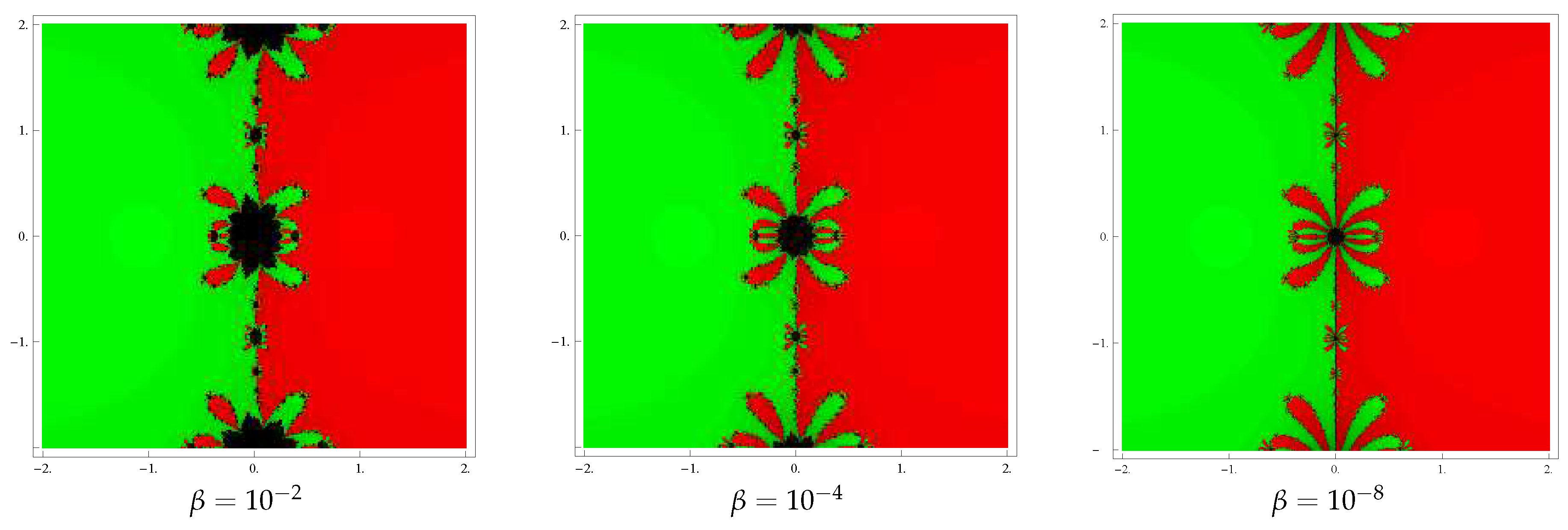
To start with we take the initial point $z_0$ in a rectangular region $R\in \mathbb{C}$ that contains all the zeros of a polynomial $P\left(z\right).$ The iterative method, when starting from point $z_0$ in a rectangle, either converges to the zero $P\left(z\right)$ or eventually diverges. Stopping condition for convergence is considered as ${10}^{-3}$ to a maximum of 25 iterations. If the required tolerance is not achieved in 25 iterations, we conclude that the iterative scheme starting at point $z_0$ does not converge to any root. The strategy adopted is as follows: A color is allocated to each initial point $z_0$ in the basin of attraction of a zero. If the iteration initiating at $z_0$ converges, then it represents the attraction basin with that assigned color to it, otherwise in the failing (divergence) situation in 25 iterations the iteration represents the black color.

We analyze the basins of attraction of the new method (for the choices $\beta ={10}^{-2},{10}^{-4},{10}^{-8}$) on following three polynomials:

Example 1.

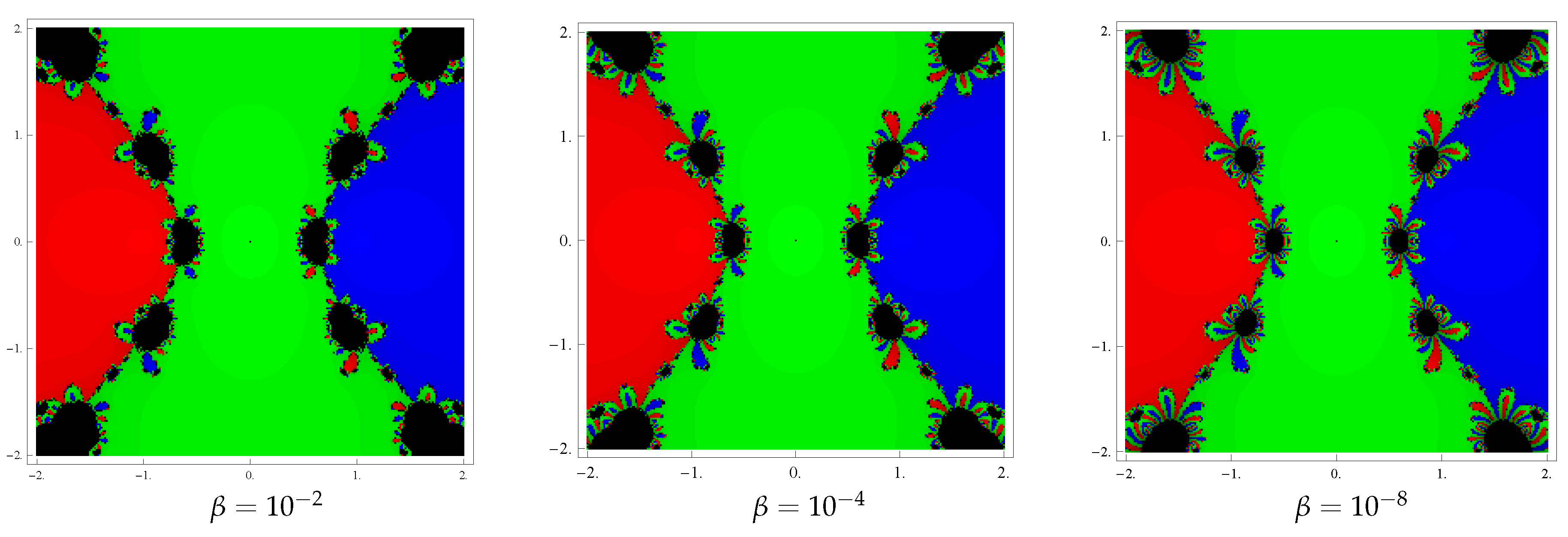
In the first case, consider the polynomial $P_1\left(z\right)=z^2-1$ which has zeros $\{\pm 1\}$. A grid of $400\times 400$ points in a rectangle $D\in \mathbb{C}$ of size $[-2,2]\times [-2,2]$ is used for drawing the graphics. We assign the color red to each initial point in the basin of attraction of zero ‘1’ and the color green to the points in the basin of attraction of zero ‘$-1$’. The graphics are shown in Figure 1 corresponding to $\beta ={10}^{-2},{10}^{-4},{10}^{-8}$. Observing the behavior of the basins of the new method, we conclude that the convergence domain becoming wider as parameter β assumes smaller values since black zones (divergent points) are getting smaller in size.

Example 2.

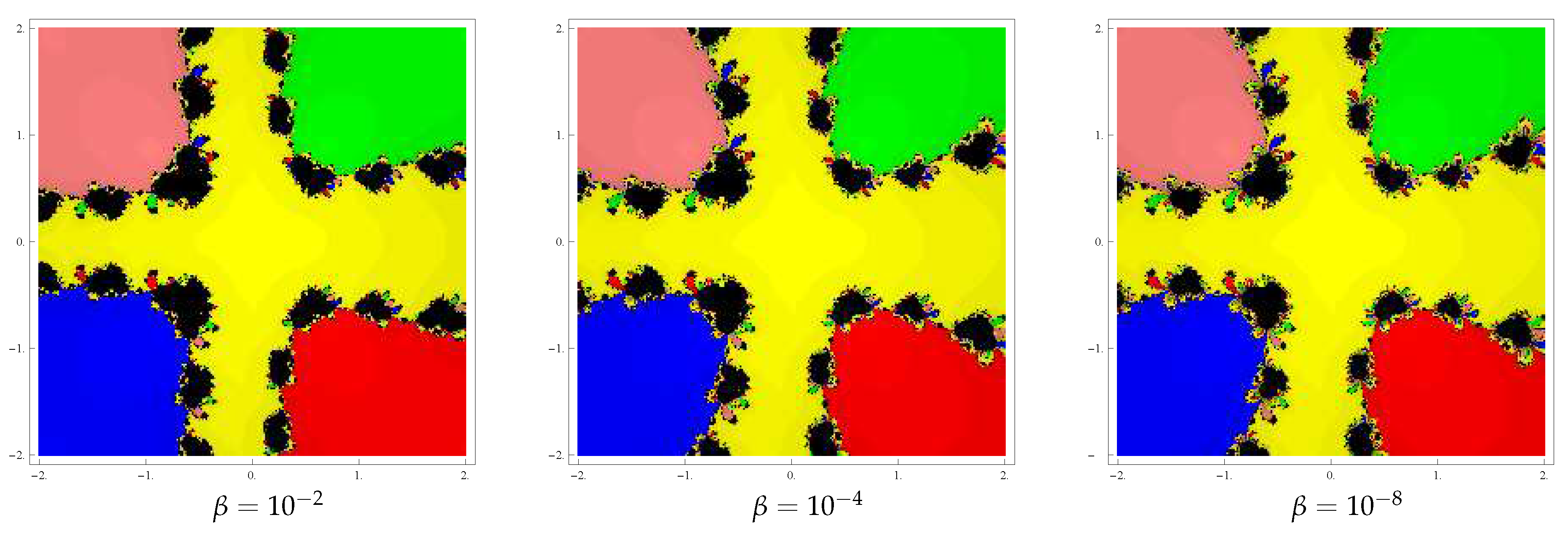
Let us consider the next polynomial as $P_2\left(z\right)=z^3-z$ having zeros $\{0,\pm 1\}$. To draw the dynamical view, we select a rectangle $D=[-2,2]\times [-2,2]\in \mathbb{C}$ containing $400\times 400$ grid points. Then, allocate the colors green, blue and red to each point in the basin of attraction of 0, 1 and $-1$, respectively. Basins for this example are exhibited in Figure 2 corresponding to parameter choices $\beta ={10}^{-2},{10}^{-4},{10}^{-8}$ in the proposed methods. In addition, observe that the basins are becoming larger and larger with the smaller values of β.

Example 3.

Lastly, we consider the polynomial as $P_3\left(z\right)=z^5+2z-1$ having zeros $\{-0.945068\pm 0.854518i,0.701874\pm 0.879697i,0.486389\}$. To draw the dynamical view, we select a rectangle $D=[-2,2]\times [-2,2]\in \mathbb{C}$ containing $400\times 400$ grid points. Then, allocate the colors green, blue, red, yellow and pink to each point in the basin of attraction of $0.701874+0.879697i$, $-0.945068-0.854518i$, $0.701874-0.879697i$, $0.486389$ and $-0.945068+0.854518i$, respectively. Basins for this example are exhibited in Figure 3 corresponding to parameter choices $\beta ={10}^{-2},{10}^{-4},{10}^{-8}$ in the proposed methods. We observe that the basins are getting larger with the smaller values of β.

6. Numerical Tests

In this section, some numerical tests on different problems are performed to demonstrate the convergence behavior and computational efficiency of the method ${\mathrm{M}}_{5,1}$. A comparison between the performance of ${\mathrm{M}}_{5,1}$ with the existing methods ${\mathrm{M}}_{2,1},{\mathrm{M}}_{3,1},{\mathrm{M}}_{4,j}(j=1,2,3)$, ${\mathrm{M}}_{5,2}$, ${\mathrm{M}}_{6,1},{\mathrm{M}}_{7,1}$ and ${\mathrm{M}}_{7,2}$ is also drawn. The programs are performed in the processor with specifications Intel (R) Core (TM) i5-4210U CPU @ 1.70 GHz 2.40 GHz (64-bit Operating System) Microsoft Windows 10 Professional and are complied by Mathematica 10.0 using multiple-precision arithmetic. We record the number of iterations $\left(k\right)$ required to converge to the solution such that the stopping condition

$$\left|\right|x^{(k+1)}-x^{\left(k\right)}\left|\right|+\left|\right|F\left(x^{\left(k\right)}\right)\left|\right|<{10}^{-300}$$

is satisfied. In order to verify the theoretical order of convergence, the computational order of convergence $\left(p_c\right)$ is obtained by using the Formula (8). In the comparison of performance of considered methods, we also include the real CPU time elapsed during the execution of program computed by the Mathematica command “TimeUsed[ ]”.

The methods ${\mathrm{M}}_{2,1}$, ${\mathrm{M}}_{3,1}$, ${\mathrm{M}}_{4,3},{\mathrm{M}}_{5,1}$ and ${\mathrm{M}}_{7,2}$ are tested by using the value $0.01$ for the parameter $\beta$. In numerical experiments we consider the following five problems:

Example 4.

Let us consider the system of two equations (selected from [29]):

$$\left\{\begin{array}{c}{x}^2+sinx-e^y=0,\hfill \\ 3x-cosx-y=0.\hfill \end{array}\right.$$

(51)

The initial guess assumed is $x^{\left(0\right)}={\{-1,-2\}}^T$ for obtaining the solution

$$\alpha ={\{-0.90743021707369569\dots ,-3.3380632251862363\dots \}}^T.$$

Example 5.

Now considering the mixed Hammerstein integral equation (see [4]):

$$x\left(s\right)=1+\frac{1}{5}{\int }_0^{1}G(s,t)x{\left(t\right)}^{3}dt,$$

wherein $x\in C[0,1]$; $s,t\in [0,1]$ and the kernel G is

$$G(s,t)=\left\{\begin{array}{c}(1-s)t,t\le s,\hfill \\ s(1-t),s\le t.\hfill \end{array}\right.$$

The above equation is transformed to a finite-dimensional problem by using the Gauss-Legendre quadrature formula

$${\int }_0^{1}f\left(t\right)dt\approx \sum _{j=1}^m{\varpi }_{j}f\left(t_j\right),$$

where the weights ${\varpi }_j$ and abscissas $t_j$ are obtained for $m=8$ by Gauss-Legendre quadrature formula. Then, setting $x\left(t_i\right)=x_i,i=1,2,\dots \dots ,8$, we obtain the following system of nonlinear equations

$$5x_i-5-\sum _{j=1}^8{a}_{ij}{x}_j^3=0,$$

where

$$a_{ij}=\left\{\begin{array}{c}{\varpi }_j{t}_j(1-t_i)ifj\le i,\hfill \\ i=1,2,\dots \dots 8.\hfill \\ {\varpi }_j{t}_i(1-t_j)ifi<j,\hfill \end{array}\right.$$

wherein the abscissas $t_j$ and the weights ${\varpi }_j$ are known and produced in

Table 1. Weights and abscissas of Gauss-Legendre quadrature formula for $m=8$.

j		${\mathit{t}}_{\mathit{j}}$		${\mathit{\varpi }}_{\mathit{j}}$
1		$0.01985507175123188415821957\dots$		$0.05061426814518812957626567\dots$
2		$0.10166676129318663020422303\dots$		$0.11119051722668723527217800\dots$
3		$0.23723379504183550709113047\dots$		$0.15685332293894364366898110\dots$
4		$0.40828267875217509753026193\dots$		$0.18134189168918099148257522\dots$
5		$0.59171732124782490246973807\dots$		$0.18134189168918099148257522\dots$
6		$0.76276620495816449290886952\dots$		$0.15685332293894364366898110\dots$
7		$0.89833323870681336979577696\dots$		$0.11119051722668723527217800\dots$
8		$0.98014492824876811584178043\dots$		$0.05061426814518812957626567\dots$

for $m=8$. The initial approximation assumed is

$$x^{\left(0\right)}={\{-1,-1,-1,-1,-1,-1,-1,-1\}}^T$$

and the solution of this problem is:

$$\begin{array}{cc}\hfill \alpha =\{& 1.002096245031\dots ,1.009900316187\dots ,1.019726960993\dots ,1.026435743030\dots ,\hfill \\ & { 1.026435743030\dots ,1.019726960993\dots ,1.009900316187\dots ,1.002096245031\dots \}}^T.\hfill \end{array}$$

Example 6.

Consider the system of 20 equations (see [29]):

$${tan}^{-1}\left(x_i\right)+1-2\sum _{j=1,j\ne i}^{20}{x}_j^2=0,1\le i\le 20,$$

This problem has the following two solutions:

$${\alpha }_1={\{0.1757683176158\dots ,0.1757683176158\dots ,\stackrel{}{·····},0.1757683176158\dots \}}^T.$$

and

$${\alpha }_2={\{-0.14968543422\dots ,-0.14968543422,\dots ,\stackrel{}{·····},-0.14968543422\dots \}}^T.$$

We intend to find the first solution and so choose the initial value: $x^{\left(0\right)}={\{0.5,0.5,0.5,\stackrel{}{·····},0.5\}}^T$.

Example 7.

Consider the boundary value problem:

$$y^{″}+y^3=0,y\left(0\right)=0,y\left(1\right)=1.$$

Assuming the following partitioning of the interval $[0,1]$:

$u_0=0<u_1<u_2<\cdots <u_{n-1}<u_n=1,u_{j+1}=u_j+h,h=1/n.$

Setting $y_0=y\left(u_0\right)=0,y_1=y\left(u_1\right),\cdots ,y_{n-1}=y\left(u_{n-1}\right),y_n=y\left(u_n\right)=1.$ If we discretize the problem by using the finite difference approximation for second derivative

$$y_m^{″}=\frac{y_{m-1}-2y_m+y_{m+1}}{h^2},m=1,2,3,\dots ,n-1,$$

we obtain a system of $n-1$ equations in $n-1$ variables:

$$y_{m-1}-2y_m+y_{m+1}+h^2{y}_m^3=0,m=1,2,3,\dots ,n-1.$$

In particular, let us solve this problem for $n=51,$ that is for $m=50$ by choosing $y^{\left(0\right)}={\{-1,-1,-1,\cdots ,-1\}}^T$ as the initial value. The solution vector α of this problem is

$$\begin{array}{c}\{0.02071138910\dots ,0.04142277479\dots ,0.06213413315\dots ,0.08284539929\dots ,0.10355644682\dots ,\\ 0.12426706739\dots ,0.14497695018\dots ,0.16568566142\dots ,0.18639262397\dots ,0.20709709683\dots ,\\ 0.22779815476\dots ,0.24849466794\dots ,0.26918528167\dots ,0.28986839623\dots ,0.31054214677\dots ,\\ 0.33120438344\dots ,0.35185265167\dots ,0.37248417270\dots ,0.39309582441\dots ,0.41368412246\dots ,\\ 0.43424520189\dots ,0.45477479913\dots ,0.47526823468\dots ,0.49572039629\dots ,0.51612572294\dots ,\\ 0.53647818972\dots ,0.55677129350\dots ,0.57699803975\dots ,0.59715093054\dots ,0.61722195374\dots ,\\ 0.63720257375\dots ,0.65708372374\dots ,0.67685579959\dots ,0.69650865572\dots ,0.71603160287\dots ,\\ 0.73541340802\dots ,0.75464229671\dots ,0.77370595761\dots ,0.79259154985\dots ,0.81128571300\dots ,\\ 0.82977457984\dots ,0.84804379222\dots ,0.86607851992\dots ,0.88386348269\dots ,0.90138297559\dots ,\\ {0.91862089765\dots ,0.93556078378\dots ,0.95218584022\dots ,0.96847898326\dots ,0.98442288125\dots \}}^T\end{array}$$

.

Example 8.

Consider the following Burger’s equation (see [30]):

$$\frac{{\partial }^{2}f}{\partial u^2}+f\frac{\partial f}{\partial u}-\frac{\partial f}{\partial t}+g(u,t)=0,(u,t)\in {[0,1]}^2,$$

where $g(u,t)=-10e^{-2t}[e^t(2-u+u^2)+10u(1-3u+2u^2)]$ and function $f=f(u,t)$ satisfies the boundary conditions

$$f(0,t)=f(1,t)=0,f(u,0)=10u(u-1)andf(u,1)=10u(u-1)/e.$$

Assuming the following partitioning of the domain ${[0,1]}^2$:

$$\begin{array}{cc}\hfill 0=& u_0<u_1<u_2<\dots \dots \dots <u_{n-1}<u_n=1,u_{k+1}=u_k+h,\hfill \\ \hfill 0=& t_0<t_1<t_2<\dots \dots \dots <t_{n-1}<t_n=1,t_{l+1}=t_l+h,h=1/n.\hfill \end{array}$$

Let us define $f_{k,l}=f(u_k,t_l)$ and $g_{k,l}=g(u_k,t_l)$ for $k,l=0,1,2,\dots \dots .n$. Then the boundary conditions would be $f_{0,l}=f(u_0,t_l)=0$, $f_{n,l}=f(u_n,t_l)=0$, $f_{k,0}=f(u_k,t_0)=10u_k(u_k-1)$ and $f_{k,n}=f(u_k,t_n)=10u_k(u_k-1)/e$. If we discretize Burger’s equation by using the numerical formulas for the partial derivatives

$${\left(\frac{\partial f}{\partial u}\right)}_{i,j}=\frac{f_{i+1,j}-f_{i-1,j}}{2h},{\left(\frac{\partial f}{\partial t}\right)}_{i,j}=\frac{f_{i,j+1}-f_{i,j-1}}{2h},$$

$${\left(\frac{{\partial }^{2}f}{\partial u^2}\right)}_{i,j}=\frac{f_{i+1,j}-2f_{i,j}+f_{i-1,j}}{h^2},i,j=1,2,\dots \dots n-1,$$

then we obtain the following system of ${(n-1)}^2$ nonlinear equations in ${(n-1)}^2$ variables:

$$f_{i-1,j}(2-h{f}_{i,j})+h(f_{i,j-1}-f_{i,j+1})-f_{i,j}(4-h{f}_{i+1,j})+2f_{i+1,j}+2h^2{g}_{i,j}=0,$$

(52)

where $i,j=1,2\dots \dots n-1$. In particular, we solve this nonlinear system for $n=11$ so that $m=100$ by selecting $f_{i,j}=1$ for $i,j=1,2\dots \dots 10$ as the initial value. The solution of this system of nonlinear equations is given in

Table 2. The solution of system (51) with the unknowns $f_{i,j}$ for $i,j=1,2,\dots \dots 10.$

${\mathit{f}}_{\mathit{i},1}$	${\mathit{f}}_{\mathit{i},2}$	${\mathit{f}}_{\mathit{i},3}$	${\mathit{f}}_{\mathit{i},4}$	${\mathit{f}}_{\mathit{i},5}$	${\mathit{f}}_{\mathit{i},6}$	${\mathit{f}}_{\mathit{i},7}$	${\mathit{f}}_{\mathit{i},8}$	${\mathit{f}}_{\mathit{i},9}$	${\mathit{f}}_{\mathit{i},10}$
$-0.7546\dots$	$-0.6892\dots$	$-0.6290\dots$	$-0.5750\dots$	$-0.5236\dots$	$-0.4817\dots$	$-0.4306\dots$	$-0.4214\dots$	$-0.2583\dots$	$-0.3068\dots$
$-1.3583\dots$	$-1.2405\dots$	$-1.1322\dots$	$-1.0351\dots$	$-0.9422\dots$	$-0.8675\dots$	$-0.7741\dots$	$-0.7598\dots$	$-0.4358\dots$	$-0.5505\dots$
$-1.8111\dots$	$-1.6541\dots$	$-1.5096\dots$	$-1.3803\dots$	$-1.2559\dots$	$-1.1573\dots$	$-1.0309\dots$	$-1.0110\dots$	$-0.6951\dots$	$-0.7356\dots$
$-2.1130\dots$	$-1.9298\dots$	$-1.7611\dots$	$-1.6106\dots$	$-1.4649\dots$	$-1.3511\dots$	$-1.2014\dots$	$-1.1768\dots$	$-0.8755\dots$	$-0.8606\dots$
$-2.2639\dots$	$-2.0678\dots$	$-1.8869\dots$	$-1.7258\dots$	$-1.5690\dots$	$-1.4485\dots$	$-1.2860\dots$	$-1.2582\dots$	$-0.9783\dots$	$-0.9244\dots$
$-2.2639\dots$	$-2.0678\dots$	$-1.8868\dots$	$-1.7261\dots$	$-1.5686\dots$	$-1.4494\dots$	$-1.2850\dots$	$-1.2558\dots$	$-1.0040\dots$	$-0.9268\dots$
$-2.1129\dots$	$-1.9300\dots$	$-1.7609\dots$	$-1.6112\dots$	$-1.4637\dots$	$-1.3534\dots$	$-1.1987\dots$	$-1.1700\dots$	$-0.9534\dots$	$-0.8672\dots$
$-1.8111\dots$	$-1.6544\dots$	$-1.5093\dots$	$-1.3812\dots$	$-1.2544\dots$	$-1.1604\dots$	$-1.0272\dots$	$-1.0010\dots$	$-0.8270\dots$	$-0.7454\dots$
$-1.3583\dots$	$-1.2408\dots$	$-1.1320\dots$	$-1.0359\dots$	$-0.9407\dots$	$-0.8704\dots$	$-0.7706\dots$	$-0.7492\dots$	$-0.6255\dots$	$-0.5609\dots$
$-0.7546\dots$	$-0.6893\dots$	$-0.6289\dots$	$-0.5755\dots$	$-0.5227\dots$	$-0.4834\dots$	$-0.4285\dots$	$-0.4152\dots$	$-0.3496\dots$	$-0.3128\dots$

.

In

Table 3. Comparison of performance of methods for Example 4.

Methods	$\left|\right|{\mathit{x}}^{\left(2\right)}-{\mathit{x}}^{\left(1\right)}\left|\right|$	$\left|\right|{\mathit{x}}^{\left(3\right)}-{\mathit{x}}^{\left(2\right)}\left|\right|$	$\left|\right|{\mathit{x}}^{\left(4\right)}-{\mathit{x}}^{\left(3\right)}\left|\right|$	k	${\mathit{p}}_{\mathit{c}}$	${\mathbf{C}}_{\mathit{p},\mathit{i}}$	${\mathbf{E}}_{\mathit{p},\mathit{i}}$	e-Time
${\mathrm{M}}_{2,1}(\beta =0.01)$	$9.94(-2)$	$4.45(-3)$	$7.14(-6)$	9	2.000	16	1.04427	0.2887
${\mathrm{M}}_{3,1}(\beta =0.01)$	$2.93(-2)$	$8.14(-6)$	$1.42(-16)$	6	3.000	22	1.05120	0.2630
${\mathrm{M}}_{4,1}$	$3.73(-4)$	$1.71(-16)$	$6.94(-66)$	5	4.000	36	1.03926	0.3234
${\mathrm{M}}_{4,2}$	$6.17(-2)$	$7.75(-7)$	$5.63(-27)$	5	4.000	36	1.03926	0.3165
${\mathrm{M}}_{4,3}(\beta =0.01)$	$5.35(-3)$	$2.42(-10)$	$7.56(-40)$	5	4.000	44	1.03201	0.3362
${\mathrm{M}}_{5,1}(\beta =0.01)$	$1.76(-3)$	$4.72(-15)$	$4.11(-73)$	4	5.000	44	1.03726	0.3297
${\mathrm{M}}_{5,2}$	$1.89(-3)$	$2.96(-15)$	$2.04(-74)$	4	5.000	52	1.03143	0.3972
${\mathrm{M}}_{6,1}$	$2.97(-2)$	$8.66(-12)$	$1.81(-69)$	4	6.000	42	1.04358	0.3120
${\mathrm{M}}_{7,1}$	$2.23(-7)$	$4.55(-52)$	$0.000$	3	7.000	56	1.03536	0.3468
${\mathrm{M}}_{7,2}(\beta =0.01)$	$7.93(-5)$	$4.14(-31)$	$3.40(-215)$	3	7.000	72	1.02740	0.4125

,

Table 4. Comparison of performance of methods for Example 5.

Methods	$\left|\right|{\mathit{x}}^{\left(2\right)}-{\mathit{x}}^{\left(1\right)}\left|\right|$	$\left|\right|{\mathit{x}}^{\left(3\right)}-{\mathit{x}}^{\left(2\right)}\left|\right|$	$\left|\right|{\mathit{x}}^{\left(4\right)}-{\mathit{x}}^{\left(3\right)}\left|\right|$	k	${\mathit{p}}_{\mathit{c}}$	${\mathbf{C}}_{\mathit{p},\mathit{i}}$	${\mathbf{E}}_{\mathit{p},\mathit{i}}$	e-Time
${\mathrm{M}}_{2,1}(\beta =0.01)$	$0.202$	$1.44(-3)$	$7.18(-8)$	9	2.000	368	1.001885	0.3437
${\mathrm{M}}_{3,1}(\beta =0.01)$	$1.73(-3)$	$1.24(-11)$	$4.56(-36)$	5	3.000	440	1.002500	0.2252
${\mathrm{M}}_{4,1}$	$0.276$	$6.19(-6)$	$1.36(-24)$	5	4.000	848	1.001636	0.3532
${\mathrm{M}}_{4,2}$	$9.94(-2)$	$4.12(-8)$	$1.23(-33)$	5	4.000	800	1.001734	0.3562
${\mathrm{M}}_{4,3}(\beta =0.01)$	$1.86(-2)$	$4.72(-11)$	$2.06(-45)$	5	4.000	816	1.001700	0.2749
${\mathrm{M}}_{5,1}(\beta =0.01)$	$1.20(-5)$	$3.49(-30)$	$7.35(-153)$	4	5.000	768	1.002098	0.2312
${\mathrm{M}}_{5,2}$	$4.50(-2)$	$1.98(-11)$	$3.74(-58)$	5	5.000	1216	1.001324	0.4234
${\mathrm{M}}_{6,1}$	$1.39(-2)$	$3.84(-17)$	$1.86(-104)$	4	6.000	872	1.002057	0.3063
${\mathrm{M}}_{7,1}$	$1.12(-2)$	$7.70(-21)$	$6.01(-148)$	4	7.000	1328	1.001467	0.3862
${\mathrm{M}}_{7,2}(\beta =0.01)$	$8.66(-5)$	$4.24(-36)$	$3.01(-255)$	4	7.000	1424	1.001367	0.3625

,

Table 5. Comparison of performance of methods for Example 6.

Methods	$\left|\right|{\mathit{x}}^{\left(2\right)}-{\mathit{x}}^{\left(1\right)}\left|\right|$	$\left|\right|{\mathit{x}}^{\left(3\right)}-{\mathit{x}}^{\left(2\right)}\left|\right|$	$\left|\right|{\mathit{x}}^{\left(4\right)}-{\mathit{x}}^{\left(3\right)}\left|\right|$	k	${\mathit{p}}_{\mathit{c}}$	${\mathbf{C}}_{\mathit{p},\mathit{i}}$	${\mathbf{E}}_{\mathit{p},\mathit{i}}$	e-Time
${\mathrm{M}}_{2,1}(\beta =0.01)$	$0.336$	$5.87(-2)$	$2.05(-3)$	10	2.000	3880	1.0001787	4.2530
${\mathrm{M}}_{3,1}(\beta =0.01)$	$0.209$	$4.29(-3)$	$6.08(-8)$	7	3.000	4300	1.0002555	3.3061
$*{\mathrm{M}}_{4,1}$	$0.370$	$2.50(-2)$	$1.37$	18	4.000	8520	1.0001627	15.469
${\mathrm{M}}_{4,2}$	$8.97(-2)$	$1.02(-5)$	$2.23(-21)$	5	4.000	8160	1.0001699	3.4542
${\mathrm{M}}_{4,3}(\beta =0.01)$	$0.133$	$2.18(-4)$	$2.85(-15)$	6	4.000	6680	1.0002076	3.8634
${\mathrm{M}}_{5,1}(\beta =0.01)$	$8.15(-2)$	$3.67(-6)$	$1.08(-27)$	5	5.000	6320	1.0002547	3.3176
${\mathrm{M}}_{5,2}$	$0.434$	$7.70(-2)$	$1.33(-2)$	7	5.000	12,400	1.0001298	7.2054
${\mathrm{M}}_{6,1}$	$3.16(-2)$	$1.38(-10)$	$1.12(-60)$	4	6.000	8580	1.0002089	3.3585
$*{\mathrm{M}}_{7,1}$	$1.572$	$3.42(-4)$	$7.60(-25)$	5	7.000	13,160	1.0001478	5.7346
${\mathrm{M}}_{7,2}(\beta =0.01)$	$1.96(-2)$	$6.66(-13)$	$3.92(-86)$	4	7.000	12,120	1.0001606	4.3594

* The methods ${\mathrm{M}}_{4,1}$ and ${\mathrm{M}}_{7,1}$ converge to the solution ${\alpha }_2$.

,

Table 6. Comparison of performance of methods for Example 7.

Methods	$\left|\right|{\mathit{x}}^{\left(2\right)}-{\mathit{x}}^{\left(1\right)}\left|\right|$	$\left|\right|{\mathit{x}}^{\left(3\right)}-{\mathit{x}}^{\left(2\right)}\left|\right|$	$\left|\right|{\mathit{x}}^{\left(4\right)}-{\mathit{x}}^{\left(3\right)}\left|\right|$	k	${\mathit{p}}_{\mathit{c}}$	${\mathbf{C}}_{\mathit{p},\mathit{i}}$	${\mathbf{E}}_{\mathit{p},\mathit{i}}$	e-Time
${\mathrm{M}}_{2,1}(\beta =0.01)$	$3.828$	$0.681$	$1.23(-2)$	9	2.000	49,200	1.00001409	0.8928
${\mathrm{M}}_{3,1}(\beta =0.01)$	$0.433$	$9.62(-5)$	$1.74(-15)$	6	3.000	51,750	1.00002123	0.7183
${\mathrm{M}}_{4,1}$	$0.840$	$9.07(-5)$	$9.18(-21)$	5	4.000	103,300	1.00001342	1.0475
${\mathrm{M}}_{4,2}$	$0.848$	$9.54(-5)$	$1.13(-20)$	5	4.000	100,900	1.00001374	1.1896
${\mathrm{M}}_{4,3}(\beta =0.01)$	$1.548$	$3.85(-3)$	$5.75(-14)$	6	4.000	66,700	1.00002078	0.8284
${\mathrm{M}}_{5,1}(\beta =0.01)$	$4.06(-2)$	$1.22(-12)$	$2.82(-65)$	4	5.000	64,300	1.00002503	0.6102
${\mathrm{M}}_{5,2}$	$8.16(-2)$	$3.64(-11)$	$7.86(-58)$	5	5.000	152,500	1.00001055	1.6563
${\mathrm{M}}_{6,1}$	$0.159$	$1.20(-11)$	$2.24(-72)$	6	6.000	103,450	1.00001732	1.0313
${\mathrm{M}}_{7,1}$	$9.92(-2)$	$1.26(-15)$	$7.09(-113)$	4	7.000	157,400	1.00001236	1.3457
${\mathrm{M}}_{7,2}(\beta =0.01)$	$0.212$	$6.80(-13)$	$3.00(-93)$	4	7.000	125,800	1.00001547	1.0938

and

Table 7. Comparison of performance of methods for Example 8.

Methods	$\left|\right|{\mathit{x}}^{\left(2\right)}-{\mathit{x}}^{\left(1\right)}\left|\right|$	$\left|\right|{\mathit{x}}^{\left(3\right)}-{\mathit{x}}^{\left(2\right)}\left|\right|$	$\left|\right|{\mathit{x}}^{\left(4\right)}-{\mathit{x}}^{\left(3\right)}\left|\right|$	k	${\mathit{p}}_{\mathit{c}}$	${\mathbf{C}}_{\mathit{p},\mathit{i}}$	${\mathbf{E}}_{\mathit{p},\mathit{i}}$	e-Time
${\mathrm{M}}_{2,1}(\beta =0.01)$	$1.980$	$1.78(-2)$	$2.66(-6)$	9	2.000	363,400	1.000001907	7.6572
${\mathrm{M}}_{3,1}(\beta =0.01)$	$0.951$	$1.31(-4)$	$4.43(-16)$	6	3.000	373,500	1.000002941	5.9846
${\mathrm{M}}_{4,1}$	$0.158$	$8.95(-8)$	$2.27(-25)$	6	2.997	746,600	1.000001471	10.503
${\mathrm{M}}_{4,2}$	$0.418$	$8.99(-6)$	$2.28(-19)$	6	3.000	736,800	1.000001491	10.249
${\mathrm{M}}_{4,3}(\beta =0.01)$	$0.453$	$5.14(-6)$	$9.22(-21)$	6	3.001	433,400	1.000002535	6.5627
${\mathrm{M}}_{5,1}(\beta =0.01)$	$0.137$	$3.08(-12)$	$3.28(-65)$	4	5.001	423,600	1.000003815	4.8255
${\mathrm{M}}_{5,2}$	$3.12(-2)$	$5.16(-13)$	$3.86(-55)$	5	3.999	1,110,000	1.000001450	10.876
${\mathrm{M}}_{6,1}$	$8.38(-2)$	$6.04(-11)$	$9.18(-46)$	5	4.001	746,900	1.000001856	9.2656
${\mathrm{M}}_{7,1}$	$1.75(-4)$	$1.74(-34)$	$4.89(-213)$	4	5.999	1,129,800	1.000001586	10.235
${\mathrm{M}}_{7,2}(\beta =0.01)$	$3.83(-3)$	$5.44(-25)$	$1.65(-155)$	4	5.996	836,600	1.000002142	8.4533

we present the numerical results produced for the methods ${\mathrm{M}}_{2,1},{\mathrm{M}}_{3,1},{\mathrm{M}}_{4,j}(j=1,2,3)$, ${\mathrm{M}}_{5,1}$, ${\mathrm{M}}_{5,2}$, ${\mathrm{M}}_{6,1}$, ${\mathrm{M}}_{7,1}$ and ${\mathrm{M}}_{7,2}$. Displayed in each table are the errors $\left|\right|x^{(k+1)}-x^{\left(k\right)}\left|\right|$ of first three consecutive approximations to corresponding solution of Examples 4–8, number of iterations $\left(k\right)$ needed to converge to the required solution, computational order of convergence $p_c$, computational cost ${\mathrm{C}}_{p,i}$, computational efficiency ${\mathrm{E}}_{p,i}$ and elapsed CPU-time (e-time) measured in seconds. In each table the meaning of $A(-h)$ is $A\times {10}^{-h}$. Numerical values of computational cost and efficiency are obtained according to the corresponding expressions given by (40)–(49). The e-time is calculated by taking the average of 50 performances of the program, where we use $\left|\right|x^{(k+1)}-x^{\left(k\right)}\left|\right|+\left|\right|F\left(x^{\left(k\right)}\right)\left|\right|<{10}^{-300}$ as the stopping condition in a single performance of the program.

From the numerical results displayed in Table 3, Table 4, Table 5, Table 6 and Table 7, it can be observed that like that of the existing methods the proposed new method shows consistent convergence behavior. Seventh order methods produce approximations with large accuracy due to their higher order of convergence, but they are less efficient. In Example 6, ${\mathrm{M}}_{4,1}$ and ${\mathrm{M}}_{7,1}$ do not converge to the required solution ${\alpha }_1$. Instead, they converge to solution ${\alpha }_2$ which is far off from initial approximation chosen. Calculation of computational order of convergence shows that the order of convergence of the new method is preserved in all the numerical examples. However, this is not true for some existing methods, e.g., ${\mathrm{M}}_{4,j}(j=1,2,3)$, ${\mathrm{M}}_{5,2}$, ${\mathrm{M}}_{6,1},{\mathrm{M}}_{7,1}$ and ${\mathrm{M}}_{7,2}$, in Example 8. Values of the efficiency index shown in the penultimate column of each table also verify the theoretical results stated in Theorem 2. The efficiency results are also in complete agreement with the CPU time utilized in the execution of the program since the method with large efficiency uses less computing time than the method with small efficiency. Moreover, the proposed method utilizes less CPU time than existing higher order methods which points to the dominance of the method. In fact, the new method is especially more efficient for large systems of nonlinear equations.

7. Conclusions

In the foregoing study, we have developed a fifth order iterative method for approximating solution of systems of nonlinear equations. The methodology is based on third order Traub-Steffensen method and further developed by using derivative free modification of classical Chebyshev’s method. The iterative scheme is totally derivative-free and so particularly suitable to those problems where derivatives are lengthy to compute. To prove the local fifth order of convergence for the new method, a development of first-order divided difference operator and direct computation by Taylor’s expansion are used.

We have examined the computational efficiency of the new method. A comparison of efficiencies with that of the existing most efficient methods is also performed. It is proved that, in general, the new algorithm is more efficient. Numerical experiments are performed and the performance is compared with existing derivative-free methods. From numerical results it has been observed that the proposed method has equal or better convergence compared to existing methods. Theoretical results related to convergence order and computational efficiency have also been verified in the considered numerical problems. Similar numerical tests, performed for a variety of other different problems, have confirmed the above drawn conclusions to a good extent.

References

1. Argyros, I.K. Quadratic equations and applications to Chandrasekhar’s and related equations. Bull. Aust. Math. Soc. 1985, 32, 275–292. [Google Scholar] [CrossRef]
2. Kelley, C.T. Iterative Methods for Linear and Nonlinear Equations; SIAM: Philadelphia, PA, USA, 1995. [Google Scholar]
3. Ostrowski, A.M. Solution of Equations and Systems of Equations; Academic Press: New York, NY, USA, 1960. [Google Scholar]
4. Ortega, J.M.; Rheinboldt, W.C. Iterative Solution of Nonlinear Equations in Several Variables; Academic Press: New York, NY, USA, 1970. [Google Scholar]
5. Potra, F.-A.; Pták, V. Nondiscrete Induction and Iterarive Processes; Pitman Publishing: Boston, MA, USA, 1984. [Google Scholar]
6. Traub, J.F. Iterative Methods for the Solution of Equations; Prentice-Hall: Englewood Cliffs, NJ, USA, 1964. [Google Scholar]
7. Ezquerro, J.A.; Hernández, M.A. An optimization of Chebyshev’s method. J. Complex. 2009, 25, 343–361. [Google Scholar] [CrossRef]
8. Argyros, I.K.; Ezquerro, J.A.; Gutiérrez, J.M.; Hernández, M.A.; Hilout, S. On the semilocal convergence of efficient Chebyshev-Secant-type methods. J. Comput. Appl. Math. 2011, 235, 3195–3206. [Google Scholar] [CrossRef]
9. Argyros, I.K.; Ren, H. Efficient Steffensen-type algorithms for solving nonlinear equations. Int. J. Comput. Math. 2013, 90, 691–704. [Google Scholar] [CrossRef]
10. Steffensen, J.F. Remarks on iteration. Skand. Aktuar Tidskr. 1933, 16, 64–72. [Google Scholar] [CrossRef]
11. Ren, H.; Wu, Q.; Bi, W. A class of two-step Steffensen type methods with fourth-order convergence. Appl. Math. Comput. 2009, 209, 206–210. [Google Scholar] [CrossRef]
12. Zheng, Q.; Zhao, P.; Huang, F. A family of fourth-order Steffensen-type methods with the applications on solving nonlinear ODEs. Appl. Math. Comput. 2011, 217, 8196–8203. [Google Scholar] [CrossRef]
13. Grau-Sánchez, M.; Noguera, M.; Amat, S. On the approximation of derivatives using divided difference operators preserving the local convergence order of iterative methods. J. Comput. Appl. Math. 2013, 237, 363–372. [Google Scholar] [CrossRef]
14. Sharma, J.R.; Arora, H. An efficient derivative free iterative method for solving systems of nonlinear equations. Appl. Anal. Discrete Math. 2013, 7, 390–403. [Google Scholar] [CrossRef] [Green Version]
15. Sharma, J.R.; Arora, H. A novel derivative free algorithm with seventh order convergence for solving systems of nonlinear equations. Numer. Algorithms 2014, 67, 917–933. [Google Scholar] [CrossRef]
16. Wang, X.; Zhang, T. A family of Steffensen type methods with seventh-order convergence. Numer. Algorithms 2013, 62, 429–444. [Google Scholar] [CrossRef]
17. Sharma, J.R.; Arora, H. Efficient higher order derivative-free multipoint methods with and without memory for systems of nonlinear equations. Int. J. Comput. Math. 2018, 95, 920–938. [Google Scholar] [CrossRef]
18. Ahmad, F.; Soleymani, F.; Haghani, F.K.; Serra-Capizzano, S. Higher order derivative-free iterative methods with and without memory for systems of nonlinear equations. Appl. Math. Comput. 2017, 314, 199–211. [Google Scholar] [CrossRef]
19. Cordero, A.; Torregrosa, J.R. Variants of Newton’s method for functions of several variables. Appl. Math. Comput. 2006, 183, 199–208. [Google Scholar] [CrossRef]
20. Genocchi, A. Relation entre la différence et la dérivée d’un même ordre quelconque. Arch. Math. Phys. I 1869, 49, 342–345. [Google Scholar]
21. Cordero, A.; Hueso, J.L.; Martínez, E.; Torregrosa, J.R. A modified Newton-Jarratt’s composition. Numer. Algorithms 2010, 55, 87–99. [Google Scholar] [CrossRef]
22. Lotfi, T.; Bakhtiari, P.; Cordero, A.; Mahdiani, K.; Torregrosa, J.R. Some new efficient multipoint iterative methods for solving nonlinear systems of equations. Int. J. Comput. Math. 2015, 92, 1921–1934. [Google Scholar] [CrossRef]
23. Krasnoselsky, M.A.; Vainikko, G.M.; Zabreiko, P.P.; Rutitskii, J.B.; Stetsenko, V.J. Approximate Solution of Operator Equations; Nauka: Moscow, Russia, 1969. (In Russian) [Google Scholar]
24. Madhu, K.; Babajee, D.K.R.; Jayaraman, J. An improvement to double-step Newton method and its multi-step version for solving system of nonlinear equations and its applications. Numer. Algorithms 2017, 74, 593–607. [Google Scholar] [CrossRef]
25. Kumar, M.; Singh, A.K.; Srivastava, A. A new fifth order derivative free Newton-type method for solving nonlinear equations. Appl. Math. Inf. Sci. 2015, 9, 1507–1513. [Google Scholar]
26. Vrscay, E.R.; Gilbert, W.J. Extraneous fixed points, basin boundaries and chaotic dynamics for Schröder and König rational iteration functions. Numer. Math. 1988, 52, 1–16. [Google Scholar] [CrossRef]
27. Varona, J.L. Graphic and numerical comparison between iterative methods. Math. Intell. 2002, 24, 37–46. [Google Scholar] [CrossRef]
28. Scott, M.; Neta, B.; Chun, C. Basin attractors for various methods. Appl. Math. Comput. 2011, 218, 2584–2599. [Google Scholar] [CrossRef]
29. Xiao, X.Y.; Yin, H.W. Increasing the order of convergence for iterative methods to solve nonlinear systems. Calcolo 2016, 53, 285–300. [Google Scholar] [CrossRef]
30. Sauer, T. Numerical Analysis, 2nd ed.; Pearson Education, Inc.: Boston, MA, USA, 2012. [Google Scholar]
Figure 1. Basins of attraction for polynomial P 1 ( z ) .
Symmetry 11 00891 g001
Figure 2. Basins of attraction for polynomial P 2 ( z ) .
Symmetry 11 00891 g002
Figure 3. Basins of attraction for polynomial P 3 ( z ) .
Symmetry 11 00891 g003