1. Introduction
In 2017, Yager proposed the concept of
q-rung orthopair fuzzy sets (
q-ROFSs) [
1], which is a generalization of intuitionistic fuzzy sets (IFSs) [
2] and Pythagorean fuzzy sets (PFSs) [
3,
4]. The
q-ROFSs are fuzzy sets in which the membership grades of an element
x are pairs of values in the unit interval,
, one of which indicates membership degree in the fuzzy set and the other nonmembership degree [
1]. For the
q-ROFSs, the membership grades need to satisfy the following conditions:
, where the parameter
q determines the range of information expression. As
q increases, the range of information expression increases. As we all known, IFSs require the condition
and PFSs require the condition
. It is obvious to observe that
q-ROFSs further diminish the restriction of IFSs and PFSs on membership grades. Therefore, compared with IFSs and PFSs,
q-ROFSs provide decision-makers more elasticity to voice opinions with respect to membership grades of an element. Recently, the
q-ROFSs have become a hotspot research topic and attracted broad attention [
5,
6,
7,
8,
9,
10,
11,
12,
13,
14,
15,
16,
17].
Graph is a convenient tool to describe the decision-making problems diagrammatically [
18]. By using this tool, the decision-making objects and their relationships are represented by vertex and edge. With different representations of decision-making information, many different types of graphs have been proposed, such as fuzzy graph [
19], intuitionistic fuzzy graph (IFG) [
20], single-valued neutrosophic graph (SVNG) [
21], intuitionistic fuzzy soft graph [
22], rough fuzzy graph [
23], Pythagorean fuzzy graph (PFG) [
24]. In consideration of the superiority of
q-ROFSs, Habib et al. [
25] proposed the concept of
q-rung orthopair fuzzy graph (
q-ROFG) based on the
q-ROFSs in 2019. The
q-ROFG is an extension of IFG [
20] and PFG [
24]. Compared with IFG and PFG,
q-ROFG has a more powerful ability to model uncertainty in decision-making problems.
Product operations on graphs are highly important part in graph theory [
26]. Many scholars have discussed product operations on different graphs. Mordeson and Peng [
27,
28,
29,
30] defined some product operations on fuzzy graphs. Later, using these operations, the degree of the vertices is obtained from two fuzzy graphs in [
31,
32]. Gong and Wang [
33] defined some product operations on fuzzy hypergraphs. Sahoo and Pal [
34] presented some product operations on IFGs and calculated the degree of a vertex in IFGs. Rashmanlou et al. [
35] proposed product operations on interval-valued fuzzy graphs and study about the degree of a vertex in interval-valued fuzzy graphs. Naz et al. [
21] discussed some product operations of SVNGs and applied SVNGs to multi-criteria decision-making. More recently, Akram et al. [
24] investigated some product operations of PFGs and the degree and total degree of a vertex in PFGs. However, the product operations on
q-ROFGs have not been researched yet, so we will pay our attention to this subject in this paper. Moreover, we have found that in SVNGs and PFGs, the results about the degree and total degree under some product operations fail to work in some cases. To improve these results, we introduced the number of adjacent vertices and obtained some more general theorems.
The reminder of this paper is organized as follows. Some notions of
q-ROFSs and
q-ROFGs are reviewed in
Section 2. The degree and total degree of a vertex in a
q-ROFG are defined in
Section 3. Some product operations on
q-ROFGs, such as direct product, Cartesian product, semi-strong product, strong product and lexicographic product, are defined, and the theorems about the degree and total degree under the defined product operations are obtained in
Section 4. Some conclusions are given in
Section 5.
3. The Degree and Total Degree
In this section, the degree and total degree of a vertex in a q-ROFG are defined.
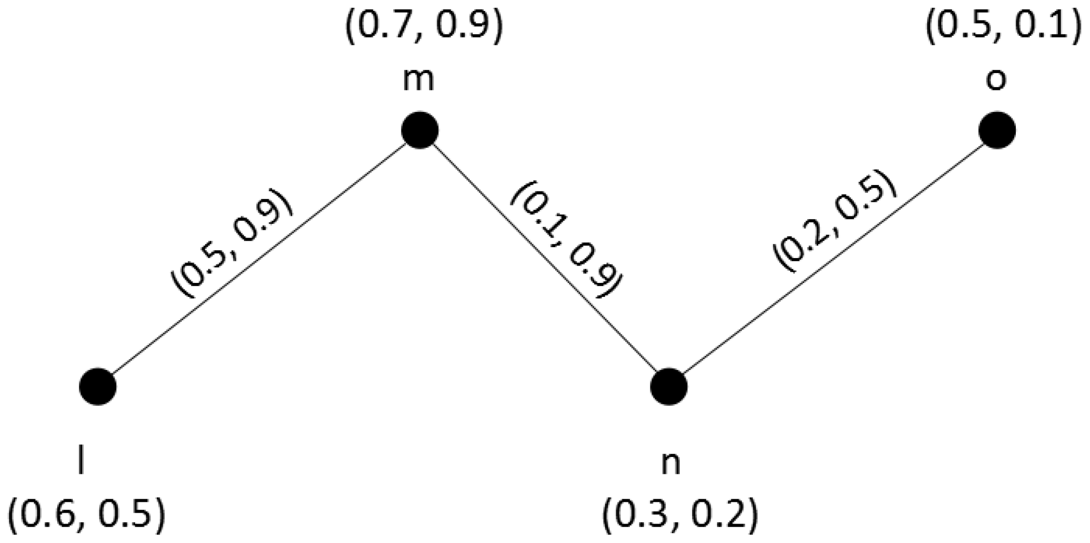
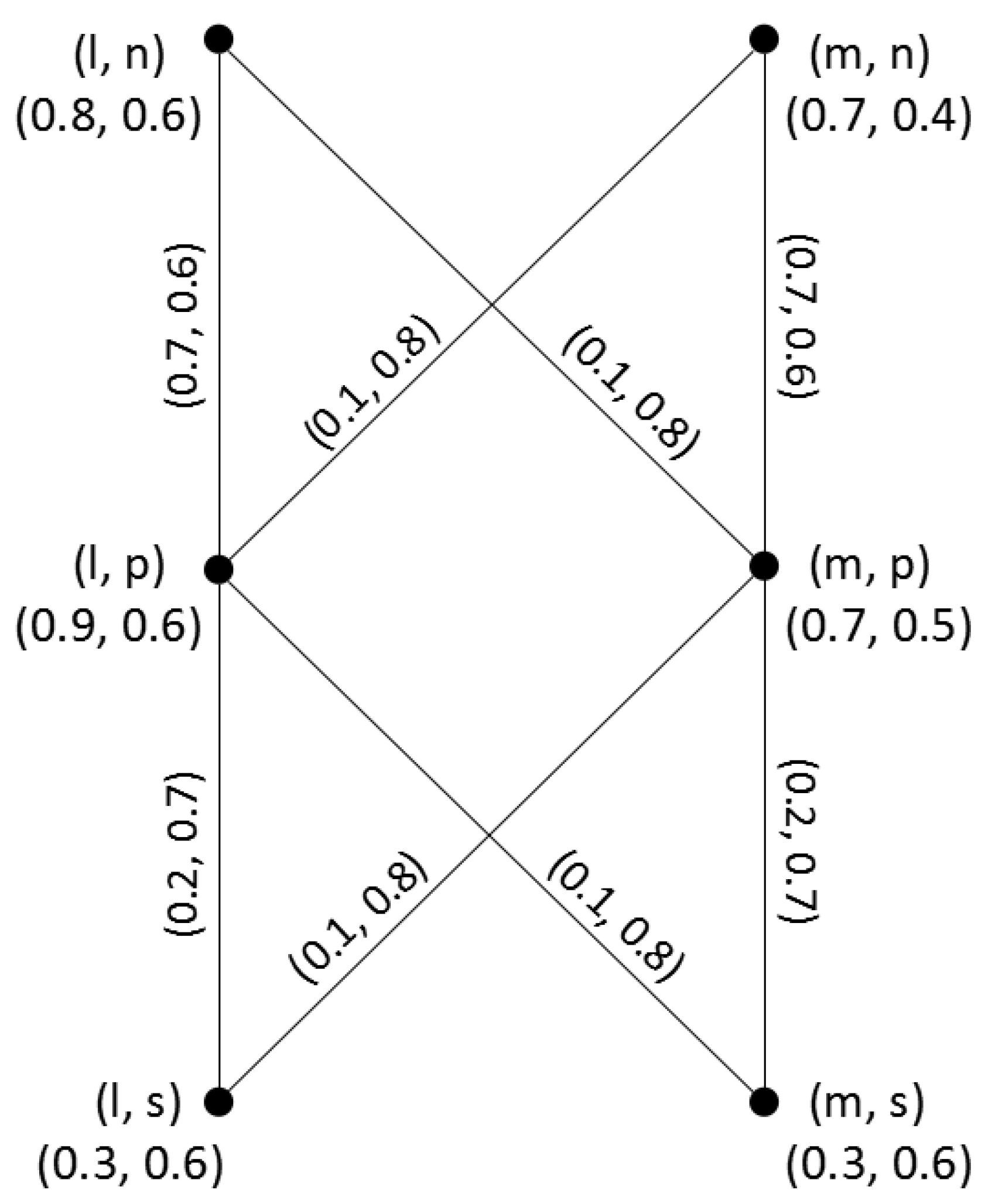
Definition 6. The degree and total degree of a vertex in a q-ROFG are defined as and , respectively, where Example 1. Considering a road network problem, there are four locations , assume that locations are performed by vertices, roads by edges, and the traffic congestion between adjacent locations is subjectively evaluated by decision-maker. The road network can be performed as a q-ROFG , where and respectively represent a q-ROFS of locations (vertices) and a q-ROFS of roads (edges). The traffic congestion of locations and roads are respectively denoted as and , see Figure 1. For example, means that the congestion degree of location l is 0.6 and the non-congestion degree of location l is 0.5. means that the congestion degree of road is 0.5 and the non-congestion degree of road is 0.9. To obtain more traffic congestion information of the road network, the degree and total degree of each location are calculated. By Definition 6, . Since , we can get . The degree of the location m represents the sum of congestion grades between m and other neighbor locations. By Definition 6, . Since , so we can get The total degree of the location m represents the sum of total congestion grades of the location m in road network. Similarly, we can obtain = (0.5, 0.9), = (1.1, 1.4), = (0.3, 1.4), = (0.6, 1.6), = (0.2, 0.5) and = (0.7, 0.6).
4. Some Product Operations on q-Rung Orthopair Fuzzy Graphs
In this section, product operations on q-ROFGs, including direct product, Cartesian product, semi-strong product, strong product and lexicographic product, are analyzed.
Definition 7. Let and be two q-ROFGs of the graphs and , respectively. The direct product of and is denoted by and defined as:
- (i)
- (ii)
Remark 1. The direct product of and can be understood that the edges of combine with the each edge of to form a new graph .
Proposition 1. Let and be the q-ROFGs of the graphs and respectively. The direct product of and is a q-ROFG.
Definition 8. Let and be two q-ROFGs. Then, for any vertex, , Theorem 1. Let and be two q-ROFGs. If then , where , represents the number of points adjacent to in and if , then for all , where represents the number of points adjacent to in .
Proof. By definition of degree of a vertex in
, we have
Hence, . Likewise, it is easy to show that if , then . □
Remark 2. In the SVNGs [21] and PFGs [24], If then . If , then (cf. Theorem 3.4 in [21] and Theorem 1 in [24]). It is obvious that they do not consider the effect of or on the degree under direct product. Definition 9. Let and be two q-ROFGs. For any vertex , Theorem 2. Let and be two q-ROFGs. For any , if
- (1)
, then ;
- (2)
, then ;
- (3)
, then ;
- (4)
, then .
In the above equalities, represents the number of points adjacent to in and represents the number of points adjacent to in .
Proof. The proof can be obtained by Definition 9 and Theorem 1. □
Remark 3. - (1)
, then ;
- (2)
, then ;
- (3)
, then ;
- (4)
, then (cf. Theorem 2 in [24]).
It is obvious that they do not consider the effect of or on the total degree under direct product.
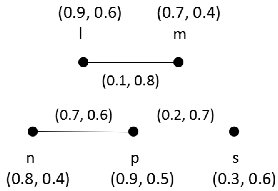
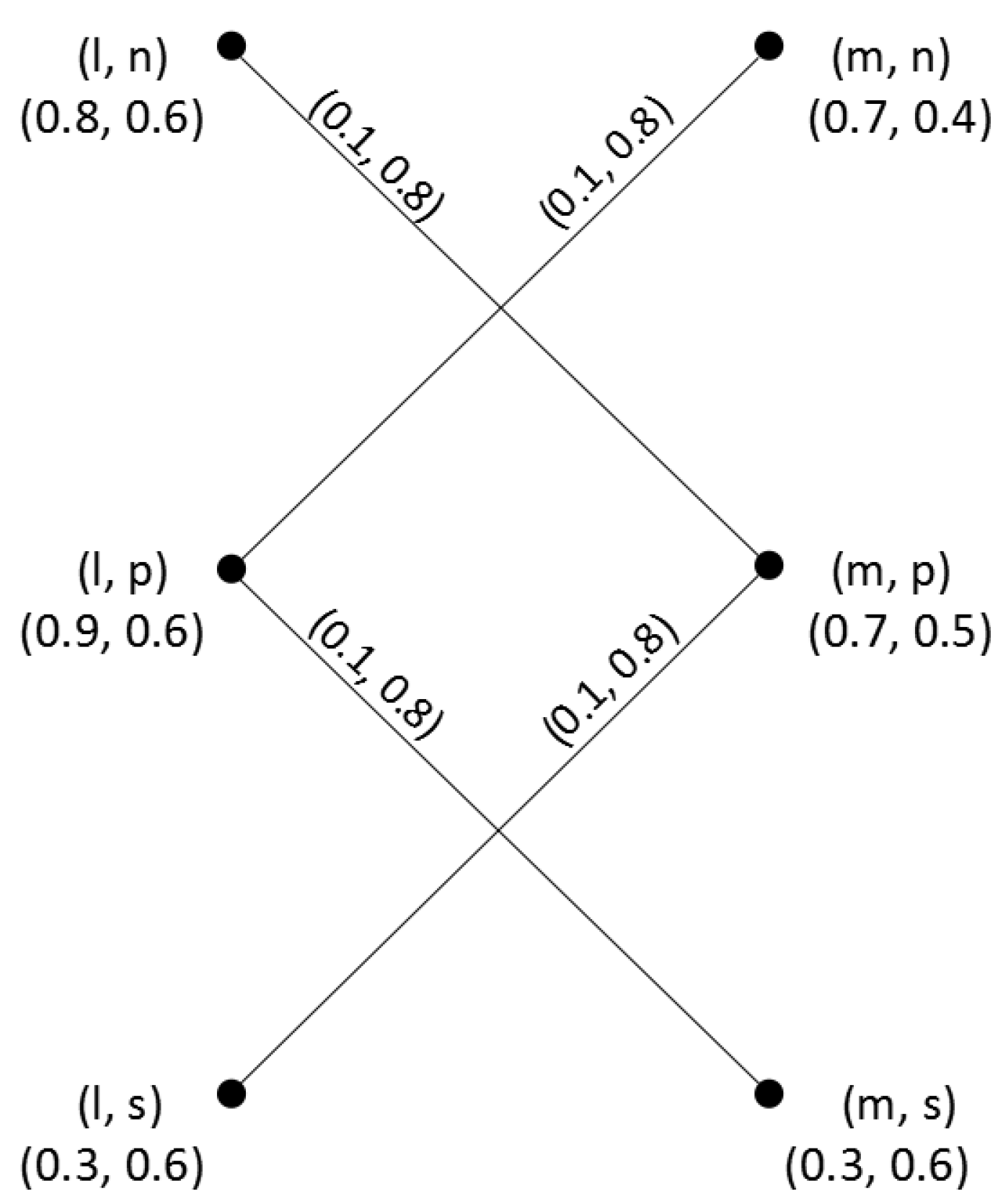
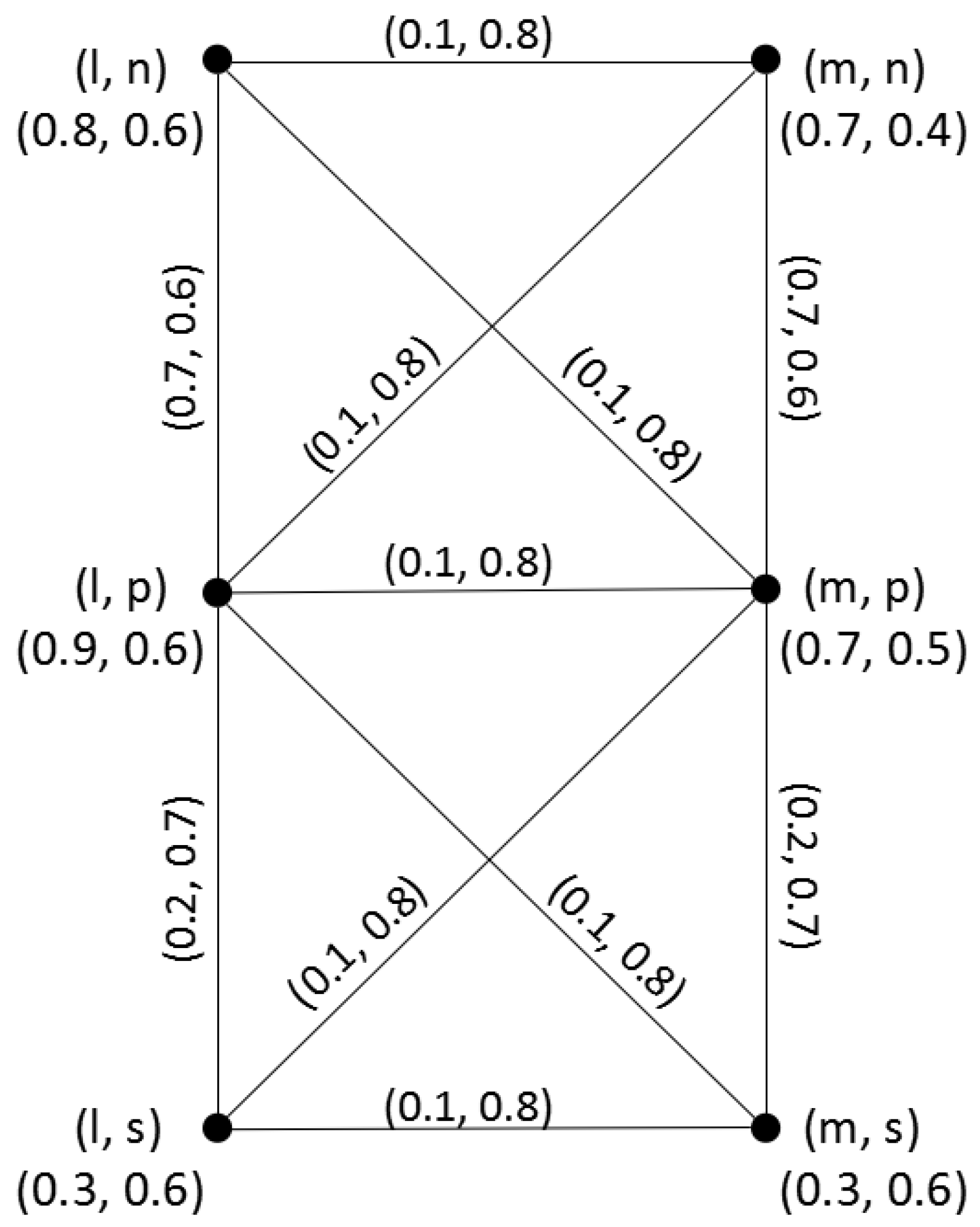
Example 2. Consider two q-ROFGs and on and , respectively, as shown in Figure 2. Their direct product is shown in Figure 3. Since , , by Theorem 1, we have Therefore, = (0.2, 1.6). In addition, by Theorem 2, we have Therefore, = (1.1, 2.2). Likewise, we can get the degree and total degree of each vertex in .
Remark 4. Klement and Mesiar [36] show that results concerning various fuzzy structures actually follow from results of ordinary fuzzy structures. These results include those from PFSs, IFSs, and many others. Although PFSs and q-rung orthopair fuzzy sets are isomorphism, Theorem 1 and Theorem 2 in this paper cannot be obtained from the results of PFGs. In the PFGs [24], they do not consider the effect of and their results fail to work in Example 2. For example, when using theorem 1 in PFGs [24], we can get However, and . When using theorem 2 in PFGs [24], we can get However, and .
Definition 10. Let and be two q-ROFGs of and , respectively. The Cartesian product of and is denoted by and defined as:
- (i)
- (ii)
- (iii)
Remark 5. The Cartesian product of and can be understood that the vertices of combine with the each edge of and the vertices of combine with the each edge of to form a new graph .
Proposition 2. Let and be the q-ROFGs of the graphs and , respectively. The Cartesian product of and is a q-ROFG.
Definition 11. Let and be two q-ROFGs. For any vertex , Theorem 3. Let and be two q-ROFGs. If and . Then for any .
Proof. By definition of degree of a vertex in
, we have
Hence, . □
Definition 12. Let and be two q-ROFGs. For any vertex , Theorem 4. Let and be two q-ROFGs. For any ,
- (1)
If , then - (2)
If , then
Proof. By definition of total degree of a vertex in
,
□
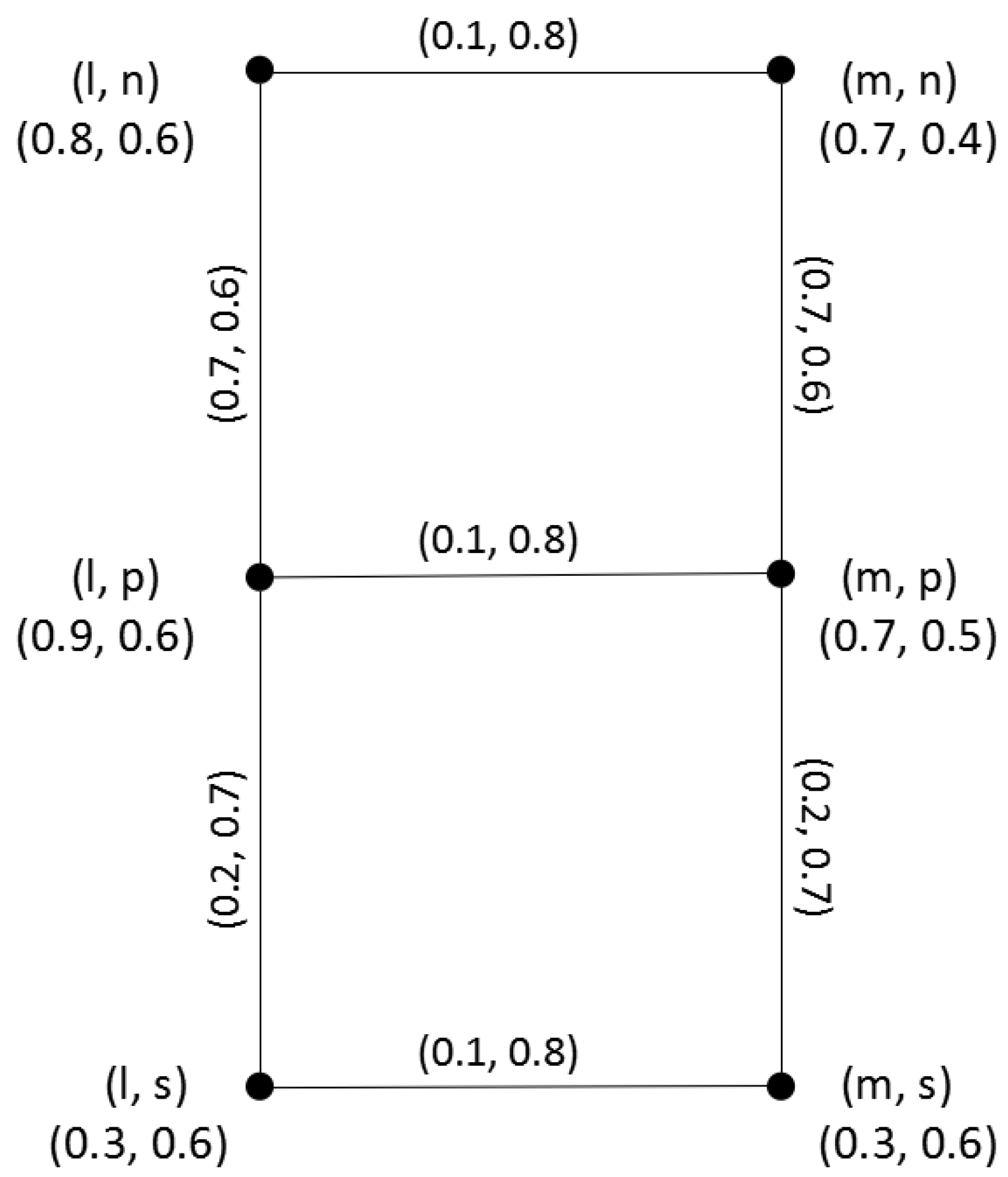
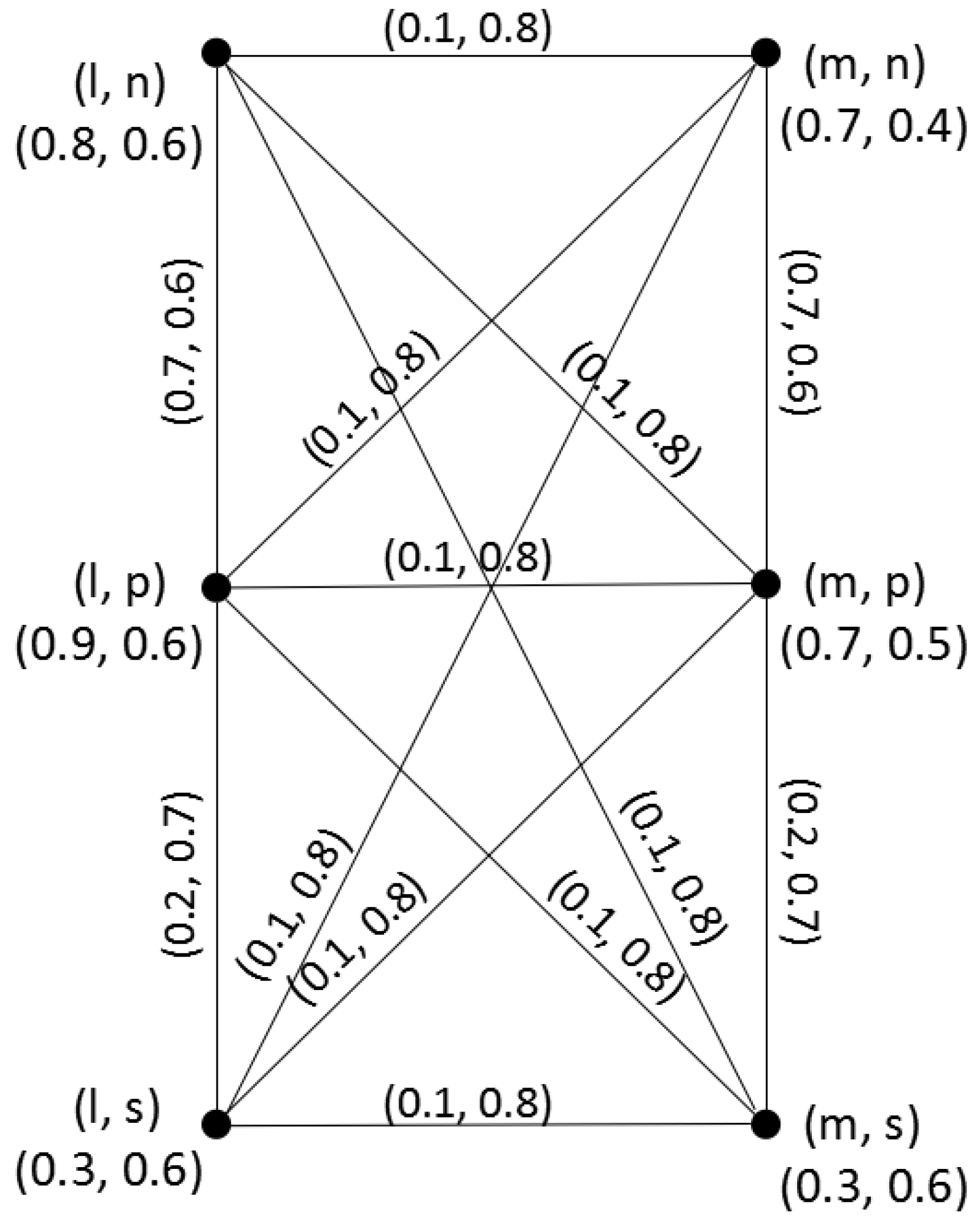
Example 3. Consider two q-ROFGs and in Example 2, where and . Their Cartesian product is shown in Figure 4. Therefore, In addition, by Theorem 4, we can get Therefore, Likewise, we can get the degree and total degree of each vertex in .
Definition 13. Let and be two q-ROFGs of the graphs and , respectively. The semi-strong product of and , denoted by , is defined as:
- (i)
- (ii)
- (iii)
Remark 6. The semi-strong product of and can be understood that the vertices of combine with the each edge of and the edges of combine with the each edge of to form a new graph .
Proposition 3. Let and be two q-ROFGs of the graphs and , respectively. The semi-strong product of and is a q-ROFG.
Definition 14. Let and be two q-ROFGs. For any vertex , Theorem 5. Let and be two q-ROFGs. If and . Then for any , where represents the number of points adjacent to in .
Proof. By definition of degree of a vertex in
, we have
Analogously, it is easy to show that . Hence, . □
Remark 7. In the SVNGs [21] and PFGs [24], if and , then (cf. Theorem 3.14 in [21] and Theorem 5 in [24]). It is obvious that they do not consider the effect of on the degree under semi-strong product. Definition 15. Let and be two q-ROFGs. For any vertex , Theorem 6. Let and be two q-ROFGs. For all ,
- (1)
If , then - (2)
If , then
In the above equalities, represents the number of points adjacent to in .
Proof. By definition 6 of total degree of a vertex in
,
Analogously, we can prove (2). □
Remark 8. In the PFGs [24], if , then ;
If , then
(cf. Theorem 6 in [24]). It is obvious that they do not consider the effect of , and on the total degree under semi-strong product.
Example 4. Consider two q-ROFGs and in Example 2, where , . Their semi-strong product is shown in Figure 5. By Theorem 5, we can getTherefore, In addition, by Theorem 6, we haveTherefore, Likewise, we can get the degree and total degree of each vertex in . Remark 9. In the PFGs [24], they do not consider the effect of and their results fail to work in Example 4. For example, when using theorem 5 in PFGs [24], we can getHowever, and . When using Theorem 6 in PFGs [24], we can getHowever, and . Definition 16. Let and be two q-ROFGs of the and , respectively. The strong product of these two q-ROFGs is denoted by and defined as:
- (i)
- (ii)
- (iii)
- (iv)
Remark 10. The strong product of and can be understood that the vertices of combine with the each edge of , the vertices of combine with the each edge of and the edges of combine with the each edge of to form a new graph .
Proposition 4. Let and be the q-ROFGs of the graphs and , respectively. The strong product of and is a q-ROFG.
Definition 17. Let and be two q-ROFGs. For any vertex , Theorem 7. Let and be two q-ROFGs. If , , , , , . Then, for all , , where represents the number of points adjacent to in .
Proof. By definition of degree of a vertex in
, we have
Analogously, it is easy to show that . Hence, . □
Remark 11. In the SVNGs [21] and PFGs [24], If , , , , , , then , where represents the number of vertices in (cf. Theorem 3.19 in [21] and Theorem 7 in [24]). It is obvious that they do not consider the effect of on the degree under strong product. Definition 18. Let and be two q-ROFGs. For any vertex , Theorem 8. Let and be two q-ROFGs. For any ,
- (1)
If , then - (2)
If , then
In the above equalities, represents the number of points adjacent to in .
Proof. For any vertex
,
Analogously, we can prove (2). □
Remark 12. In the PFGs [24], if , then ;
If , then
(cf. Theorem 8 in [24]). It is obvious that they do not consider the effect of on the total degree under strong product.
Example 5. Consider two q-ROFGs and in Example 2, where , and their strong product is shown in Figure 6. By Theorem 7, we haveTherefore, In addition, by Theorem 8, we haveTherefore, Likewise, we can find the degree and total degree of each vertex in . Remark 13. In the PFGs [24], they do not consider the effect of . For example, when using theorem 7 in PFGs [24], we can getWhen using theorem 8 in PFGs [24], we can getAlthough they get the same values as the Example 5, but the variable means different things. is represented by number of points in . Actually, should be replaced by in Example 5. Definition 19. Let and be two q-ROFGs of the and , respectively. The lexicographic product of these two q-ROFGs is denoted by and defined as follows:
- (i)
- (ii)
- (iii)
- (iv)
Remark 14. The lexicographic product of and can be understood that the vertices of combine with the each edge of , the vertices of combine with the each edge of and the edges of combine with the two different vertices of to form a new graph .
Proposition 5. The lexicographic product of two q-ROFGs of and is a q-ROFG.
Definition 20. Let and be two q-ROFGs. For any vertex , Theorem 9. Let and be two q-ROFGs. If and . Then, , for any , where represents the number of vertices in .
Proof. For any vertex
,
Analogously, we can show that Hence, □
Definition 21. Let and be two q-ROFGs. For any vertex , Theorem 10. Let and be two q-ROFGs. For any ,
- (1)
If , then - (2)
If , then
In the above equalities, represents the number of vertices in .
Proof. For any vertex
,
Analogously, we can prove (2). □
Example 6. Consider two q-ROFGs and in Example 2, where and and their lexicographic product is shown in Figure 7. Therefore, In addition, by Theorem 10, we must have Therefore, Likewise, we can get the degree and total degree of each vertex in .


