1. Introduction
Successive global influenza pandemics have attracted a great deal of attention from society and public heath officials. For instance, in the early 2000s, the dangerous avian influenza H5N1 strain jumped from poultry in Southeast Asia to humans and caused a serious pandemic outbreak (Abbott and Pearson [
1], Ferguson et al. [
2]). In 2009, the H1N1 influenza virus (“swine flu”) emerged as a worldwide outbreak (see, for instance, Andradóttir et al. [
3]).
Disease outbreaks continue to be a major concern. For this reason, detailed study of influenza and other diseases is needed to help public policymakers with respect to the identification and control of such pandemics, and to evaluate pandemic preparedness plans. Various techniques have been developed over the years to do so. These techniques are often based on models involving differential equations or computer simulation.
In typical disease propagation models, as time progresses, individuals in a population make transitions from one health state to another according to a given rate or probability distribution. The most-basic disease spread model is what is known as the
SIR model (Kermack and McKendrick [
4]). At any time
t, each individual must be either susceptible (S), infected (I), or removed (R), where “removed” means that the individual has either recovered or is dead, and will not be infected again; and it is only possible to move from S to I to R. If we let the quantities
,
, and
denote the numbers of individuals in states S, I, and R, respectively, at time
t, then the instantaneous transition rates from one state to another are given by a set of simple differential equations:
where
and
denote the infection and recovery rates. Thus, for instance,
is the overall rate at which the population transitions from state S to state I. These classical equations can be used to model the number of individuals in each state at any time, as well as the probability that any individual will make a particular transition.
There is a rich literature of models based on differential equations, and these are widely accepted in the field. Some minor issues with these models concern the facts that they tend to perform poorly in small-population settings (where, notably, the numbers of individuals in each state much be integers); they usually do not take randomness into account; and they do not easily accommodate or study individual-level behavior.
A complementary simulation-based pandemic modeling literature has arisen to address some of the issues outlined above. Simulation is especially attractive due to the complex modeling issues that arise in the study of pandemics. For instance, what are the effects of the demographic composition of the population? How can intervention strategies such as vaccination or social distancing best be applied? Under what circumstances should we close a school as an intervention strategy? See, e.g., the papers Andradóttir et al. [
3], Elveback et al. [
5], Halloran et al. [
6], Kelso et al. [
7], Lee et al. [
8], and Longini et al. [
9,
10] for additional background, motivation, and insights. Each of these papers uses a discrete-event / agent-based simulation approach, where individuals come into contact with each other on a daily basis at home, school, work, or outside of work (“compartments”). Potential criticisms of this approach are that (i) the models simulating daily life are often quite complicated (and are a bit of an art to develop); (ii) they produce “random” output; and (iii) the simulations may sometimes involve a tremendous amount of computation to complete.
In terms of potential drawback (i), it has come to pass that the use of simulation to model pandemic disease spread is now widely accepted, even if some of the modeling elements are sometimes regarded as ad hoc. To address this latter issue, there has been a great deal of work in the literature that incorporates sophisticated population modeling techniques—including population mixing and movement of individuals from location to location—along with a variety of mitigation strategies; see Andradóttir et al. [
11] for additional motivation and references. With respect to (ii), one simply simulates any particular scenario over many independent replications and then conducts what can be regarded as standard, run-of-the-mill data analysis on the independent outputs. Our concern in this article is with simulation efficiency, item (iii).
With issue (iii) in mind, we discuss the simulation of a somewhat simplified version of the SIR model. Suppose that each susceptible individual may encounter each infected individual at most once a day. At such an encounter, the probability that the susceptible will become infected is p, and we assume that all encounters are independent so that each encounter is a Bernoulli trial. In some models, infected subjects first undergo a latent (noninfectious) period before actually become infectious; but for ease of exposition, the current paper will subsequently ignore that additional state. On any given day, individuals may move between contact groups (e.g., home, school, work, etc.), thereby encountering multiple cliques of people as the day goes on. A realization of the simulation usually proceeds until either no more susceptible individuals remain (only states I and R) or no more infected individuals remain (only states S and R), indicating that the disease has run its course. Moreover, the simulation is run over multiple independent replications, so as to obtain statistically sound estimates of system performance measures such as the expected number of individuals who are ultimately infected, the peak number of people infected over the course of the outbreak, and the expected length of the pandemic.
A critical driver of computational effort is the number of Bern(
p) trials that need to be carried out; this effort grows quickly as the population size increases and is an underlying concern of the current paper.
Section 2 discusses how these trials are implemented, as well as some tricks that can be used to ameliorate the work effort. In particular, we propose the use of “green” simulation, in which we reuse many of the Bern(
p) trials between certain runs, thus avoiding recalculation effort (see, e.g., Feng and Staum [
12] and Meterelliyioz et al. [
13], the former of which coined the term). This is the main contribution of our article.
Section 3 presents several simple examples illustrating the method’s efficacy. We also show how to use the methodology for purposes of sensitivity analysis—e.g., what is the derivative of the expected number of infected individuals as a function of
p? The latter application combines a simulation variance reduction technique (see Law [
14]) with our green technology.
Section 4 provides conclusions in addition to various potential augmentations of future interest.
2. Efficient Bernoulli Generation
A naive simulation of disease propagation would require us to generate a Bernoulli trial each time a susceptible individual (heretofore referred to as a “susceptible”) were to come in contact with an infected individual (an “infective”), for every replication of every experimental design point. Of course, a single Bern(p) trial merely requires that the simulation generates a Unif(0,1) pseudo-random number (PRN) U; and if , then the interpretation is that the susceptible becomes infected. However, the problem is that the entire exercise may require a tremendous number of Bern(p) trials, a task which eventually becomes costly with respect to computer time.
What might one do to reduce the computational effort involving Bernoulli trials? There are a number of useful tricks, depending on the situation:
Within a particular simulation run, one could use a
binomial random variable instead of a series of Bern(
p) random variables to determine the number of new infections. For instance, if an infective walks into a room with
n susceptibles, and
is “small,” then it may more efficient to (i) generate one Bin(
) random variate
X representing in one fell swoop the number of susceptibles who will become infected than to instead (ii) sample
n individual Bern(
p) trials corresponding to the
n susceptibles. If one were to take the Bin(
) route, one could sample a single Unif(0,1) PRN and use the discrete distribution version of the inverse-transform method to do a table look-up or instead use a normal distribution approximation to the binomial to generate the corresponding value for
X (see, e.g., Law [
14]). If
, we would then have to randomly reassign
x susceptibles to the infected state, which would take a little bit more work—though the expected number of assignments is only
.
Within a particular simulation run, we could work with a single “super-infective” individual rather than multiple infectives. Consider the scenario above, except that
k infectives walk into the room containing
n susceptibles. Assuming that all of the infectives interact with all of the susceptibles in the form of Bern(
p) trials, an easy calculation shows that the probability that a particular susceptible will become infected that day is
, where
. Then, instead of performing
Bern(
p) trials with the individual infectives, we might equivalently perform only
n Bern(
) trials using a“super-infective” entity—or even a single Bin(
) trial; see
Section 4 or references such as Tsai et al. [
15].
Consider driving the simulation from different points of view. For example, is it more efficient to (i) generate each infected individual and see which susceptibles he infects as he proceeds through his day, or (ii) generate each susceptible individual and see if he gets infected as he proceeds through his day? See Shen et al. [
16] and Tsai et al. [
15] for insights and recommendations.
When re-running a simulation but with different input parameters, we might reuse from one simulation to the next as many of the random numbers as possible. This is the goal of the current paper. To illustrate, again consider the situation in which one infectious individual walks into a room with n susceptibles. Suppose that we perform n Bern() trials to determine who, if anyone, becomes infected. Now suppose we run another simulation, but this time with a new probability of infection . We will show how to reuse many of the PRNs from the initial simulation to do the version of the job with less effort.
In what follows, we illustrate the workings of the “green” reuse of PRNs. We begin with a baseline example in which, on any given day, each infective has probability of infecting any remaining susceptible. The simulation begins with infected person and susceptibles at the end of Day 0 / beginning of Day 1. The number of infectives at the beginning of Day t is , and the probability that any particular susceptible will be infected by at least one of those infectives is , as explained in Item 2 above. The numbers of individuals in states S, I, and R at the end of day t are , , and , respectively. Bern() trials are conducted until no infectives remain. Infectives stay infectious for exactly one day, whereupon they transit to the removed state.
Table 1 keeps track of one realization of the simulation. Day 1 starts with
Bern(0.2) trials, since there is
infective entering the room full of susceptibles. Any susceptible corresponding to a PRN
becomes infected. For instance, the PRN for individual 6 is 0.082, so he transits to state I; and subsequent Bernoulli trials will no longer be necessary for him. At the end of Day 1, we have
remaining susceptibles,
newly infectious people, and
removed people (the original infected “person 0” is no longer infected, but we will not count him in the
tally). On Day 2, we only need to take 12 Bern(0.488) trials, where
. On Day 2, e.g., individual 3 becomes infected since his PRN =
. The exercise continues until Day 5, whereupon no infectives remain. In total, the pandemic lasted five days, 14 people were infected, and we used 37 PRNs.
Table 2 illustrates the corresponding “green” realization of the simulation, using the same PRNs as those in
Table 1, but with the new probability
that an infectious individual will infect any particular susceptible. Day 1 now starts with
Bern(0.3) trials, since there is again
infective entering the room full of susceptibles. Thus, in this case, any susceptible corresponding to a PRN
becomes infected. In this riskier environment, seven Bern(0.3) trials—using the same PRNs as before—result in an infection, so subsequent Bernoulli trials will no longer be necessary for those individuals. At the end of Day 1, we have
remaining susceptibles,
newly infectious people, and
removed people. On Day 2, we only need to take seven Bern(0.91765) trials, where
. Since the pandemic progresses more rapidly, we now stop at Day 4, when no new state changes can occur. In total, the pandemic lasted four days, all 15 people were infected, and we used 24 PRNs (which themselves had already been generated for the previous
Table 1 version of the example).
Remark 1. A number of comments are in order here:
Generally speaking, the pandemic progresses quickly if p is very small (in which case the pandemic dies out rapidly) or very large (in which case the pandemic rapidly infects many people). Thus, for p very small or very large, we would expect to use only a small number of PRNs. Intermediate values of p might require more PRNs. See Section 3, Example 1. How many PRNs will we need to generate in order to simulate multiple scenarios involving the same n susceptible individuals, with each scenario having a different parameter value, for instance, ? With Remark 1.1 in mind, it might be prudent to generate an initial set of PRNs for possible use in any of the scenarios, where T is the maximum time horizon of interest. It is almost certain that many of the PRNs will never be used if, e.g., T is conservatively chosen to be so high as to guarantee that the pandemic will have run its course. However, if we are running a large number of scenarios, then the expected savings garnered by the use of green simulation would likely mitigate the conservativeness of T and the corresponding one-time charge of generating PRNs. For example, for the scenarios presented in Table 1 and Table 2, the maximum possible number of days for the scenarios to run is 15, in which case would be a conservative choice. See Section 4 for more insight on this matter. It is possible (in rare cases) to obtain sample paths in which an individual becomes infectious on a certain day when simulating the Bernoulli trials for a particular probability parameter , but remains susceptible on that day when the simulation is re-run under a scenario with a larger probability parameter . For such an anomalous example, see the sample paths of Individual 3 in Table 3 and Table 4 for the cases and 0.25, respectively; and see Section 4 for additional discussion.
3. Examples
With the mechanics of the methodology established, we put forth in this section a series of examples to assess the performance of the proposed green method, including its efficiency as compared to traditional (naive) simulation. Examples 1 and 2 in
Section 3.1 give exact small-sample results that allow us to succinctly see how various system performance characteristics (e.g., the expected number of individuals infected and the expected length of the pandemic) are affected as the Bernoulli
p parameter varies. Although these sorts of results are interesting in and of themselves, they also provide partial validation for the subsequent simulations that we will run. Such exact results might even allow us to avoid simulation altogether—but only for extremely small population sizes. Example 3 in
Section 3.2 is concerned with a cohort size (
susceptibles) that is large enough so that we are forced to use simulation to assess system performance as we vary
p. This example is useful for indicating what typical histograms might look like for the system performance characteristics of interest. Finally,
Section 3.3 presents a number of results that directly address the contibutions of our green simulation technology. Namely, Example 4 uses simulation to establish run-time savings on a larger, more-complicated scenario involving a cohort of size
; and Example 5 illustrates how we can use simulation variance reduction methods to conduct certain sensitivity analyses on the various performance characteristics.
3.1. Some Small-Sample Exact Results
First of all, it is natural to ask if it is possible to obtain exact analytical results for the problem at hand using only elementary combinatoric arguments. Indeed, one can sometimes carry out the necessary calculations, though these soon become too tedious even for very small problem instances.
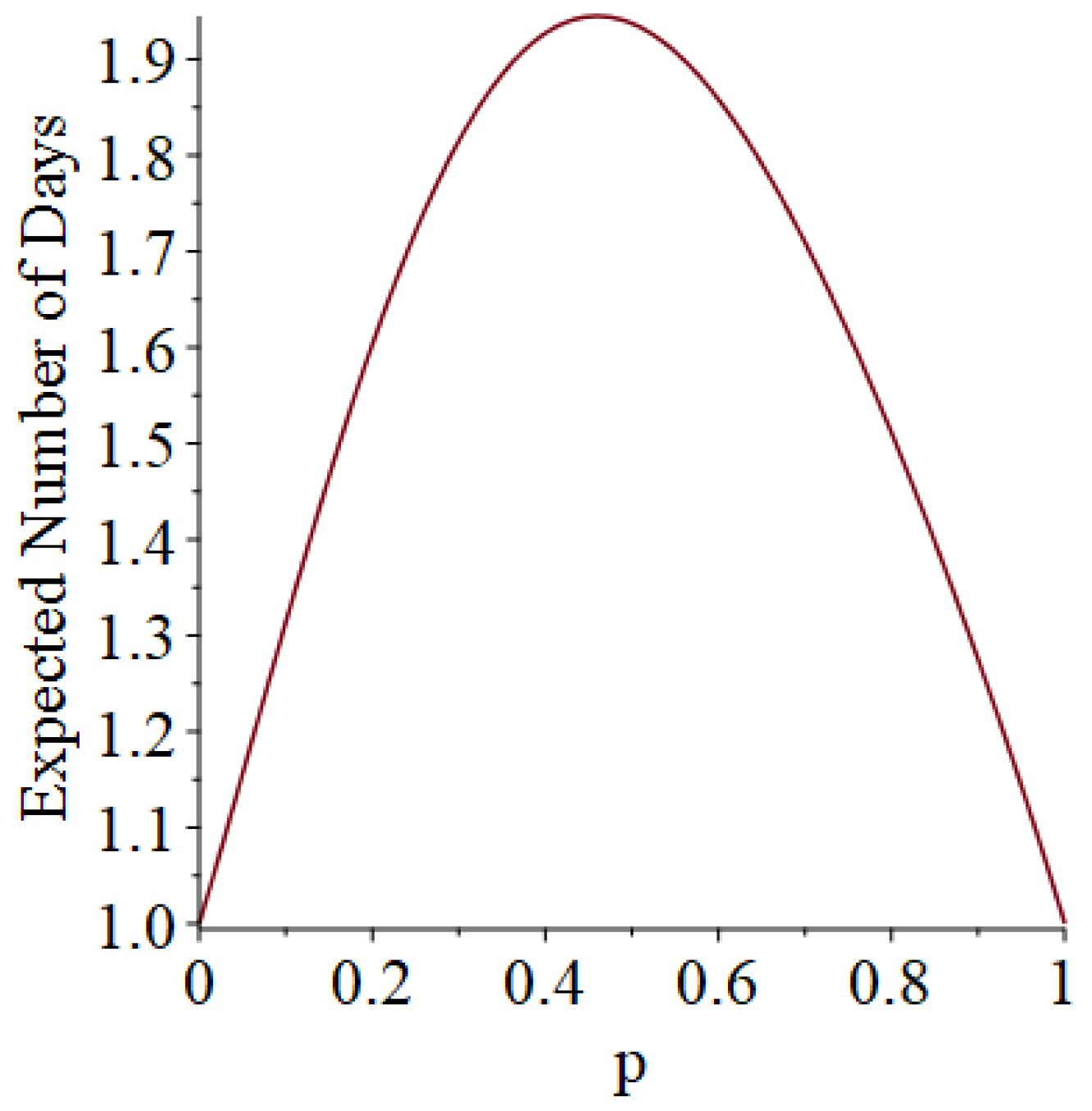
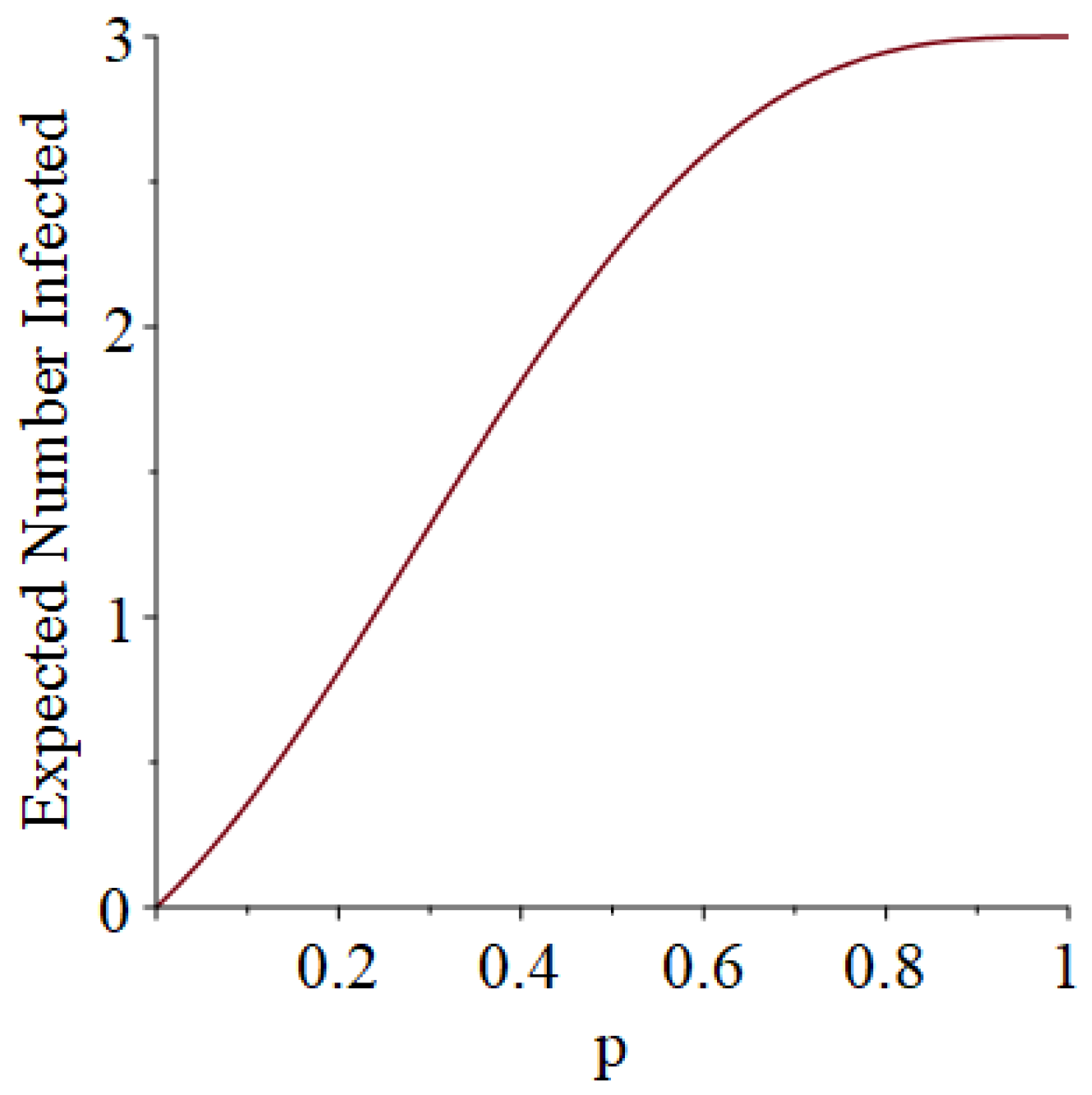
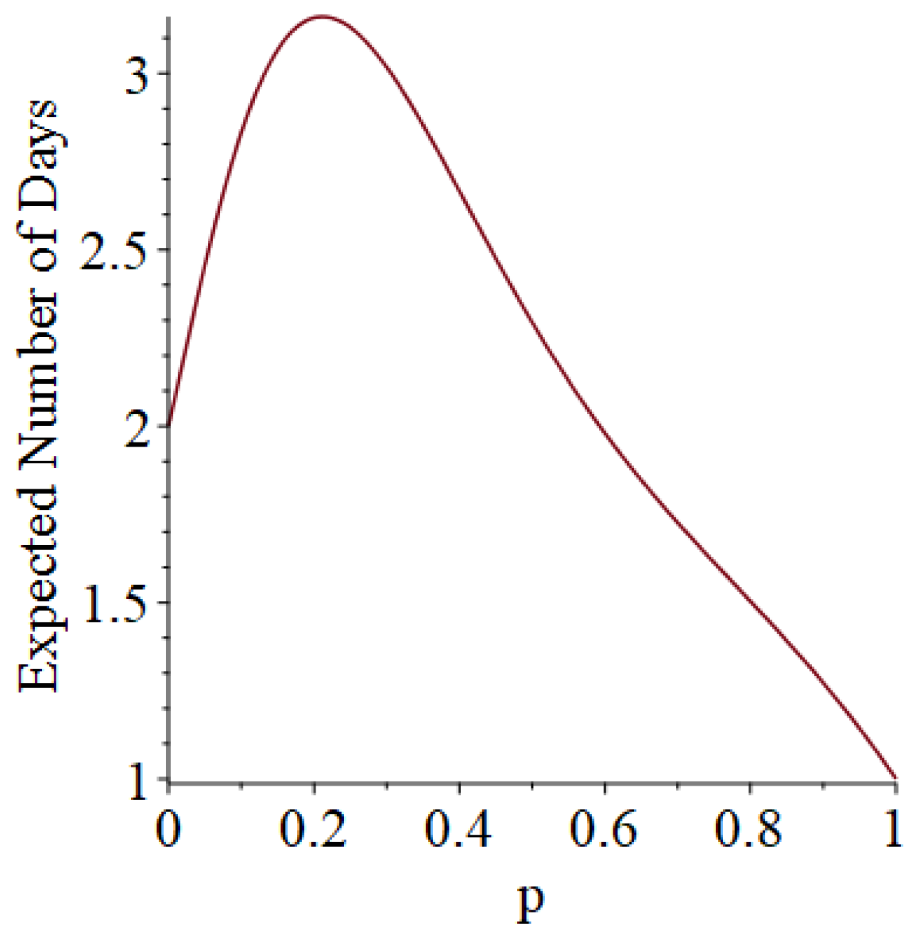
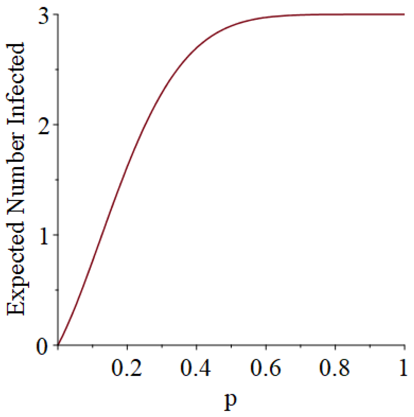
Example 1. Suppose that susceptibles are in a room, and they are exposed to one infective on Day 1. Moreover, suppose that each infective stays infectious for exactly one day (so that he only has one chance to infect his friends). Let D denote the length of the pandemic (i.e., how long the pandemic lasts until no infectives remain). In addition, let I denote the number of people who ultimately get infected (not counting person 0). Then, some slightly tedious calculations (algebra not shown) reveal thatandSee Figure 1 and Figure 2, which respectively illustrate the expected length of the outbreak and the expected number of individuals ultimately infected. Let B denote the number of Bernoulli trial comparisons that would have to be made in a simulation of this scenario, where we use the “super-infective” trick described in Item 2 of Section 2. That is, B is the total number of days all of the susceptibles will be exposed to potential infection during the course of the pandemic. (The quantity B informally represents the simulation effort we would have to undertake.) Then, it turns out that Example 2. Suppose that susceptibles are in a room, and they are exposed to one infective on Day 1. However, now, each infective stays infectious for exactly two days (so that he gets two chances to infect his friends). Then, after a corvée of tedious calculations, we obtainandSee Figure 3 and Figure 4. 3.2. Simulation
It ought to be clear from Examples 1 and 2 in
Section 3.1 that even small-sample exact calculations present combinatorial challenges. Luckily, it is easy to carry out simulations for more-substantive examples involving larger values of the cohort size
n. In this section, we consider a simple example involving a non-trivial cohort size so as to illustrate what typical disease characteristic histograms might look like for moderate values of
n, in particular, as we vary the infectiousness parameter
p.
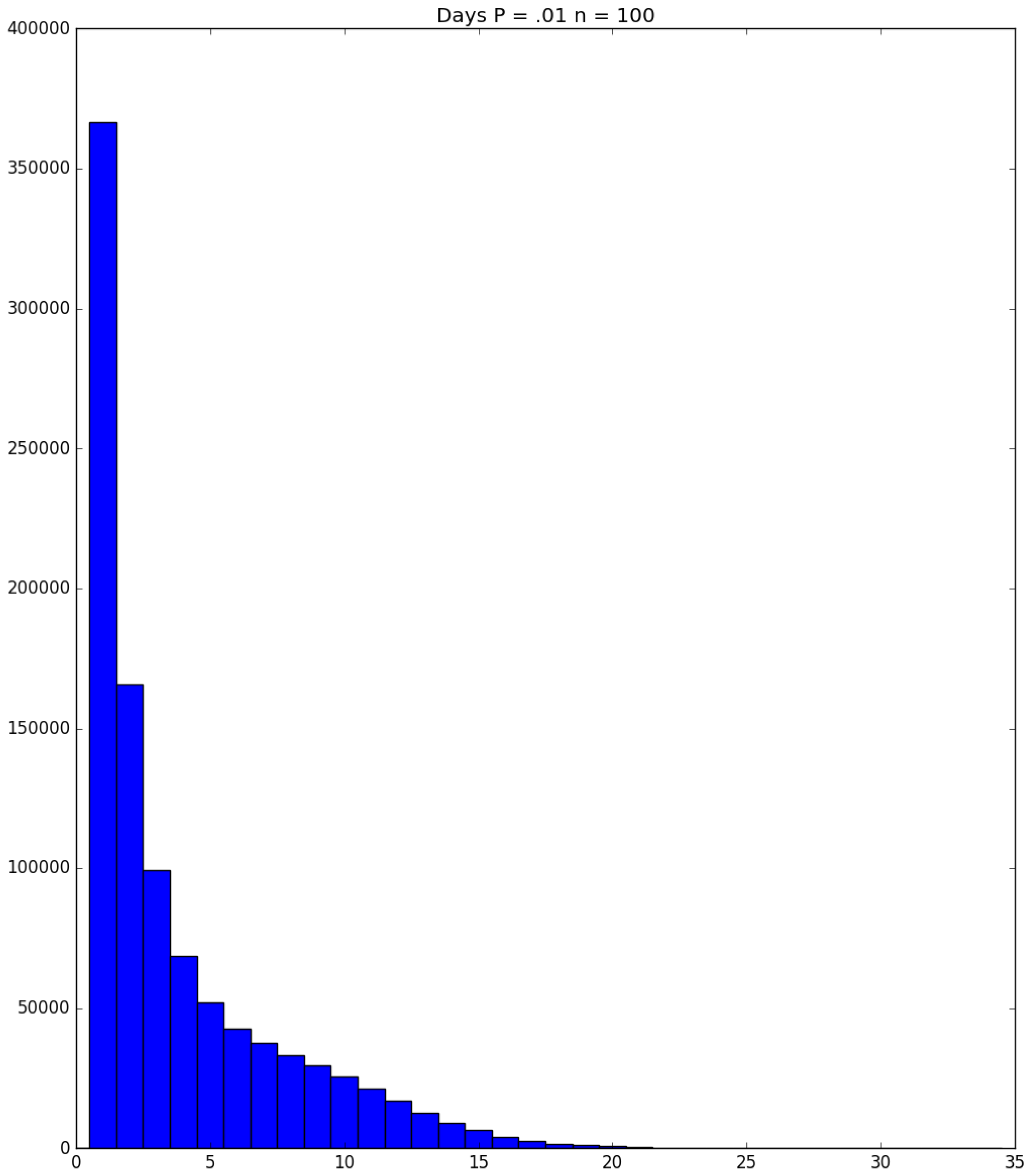
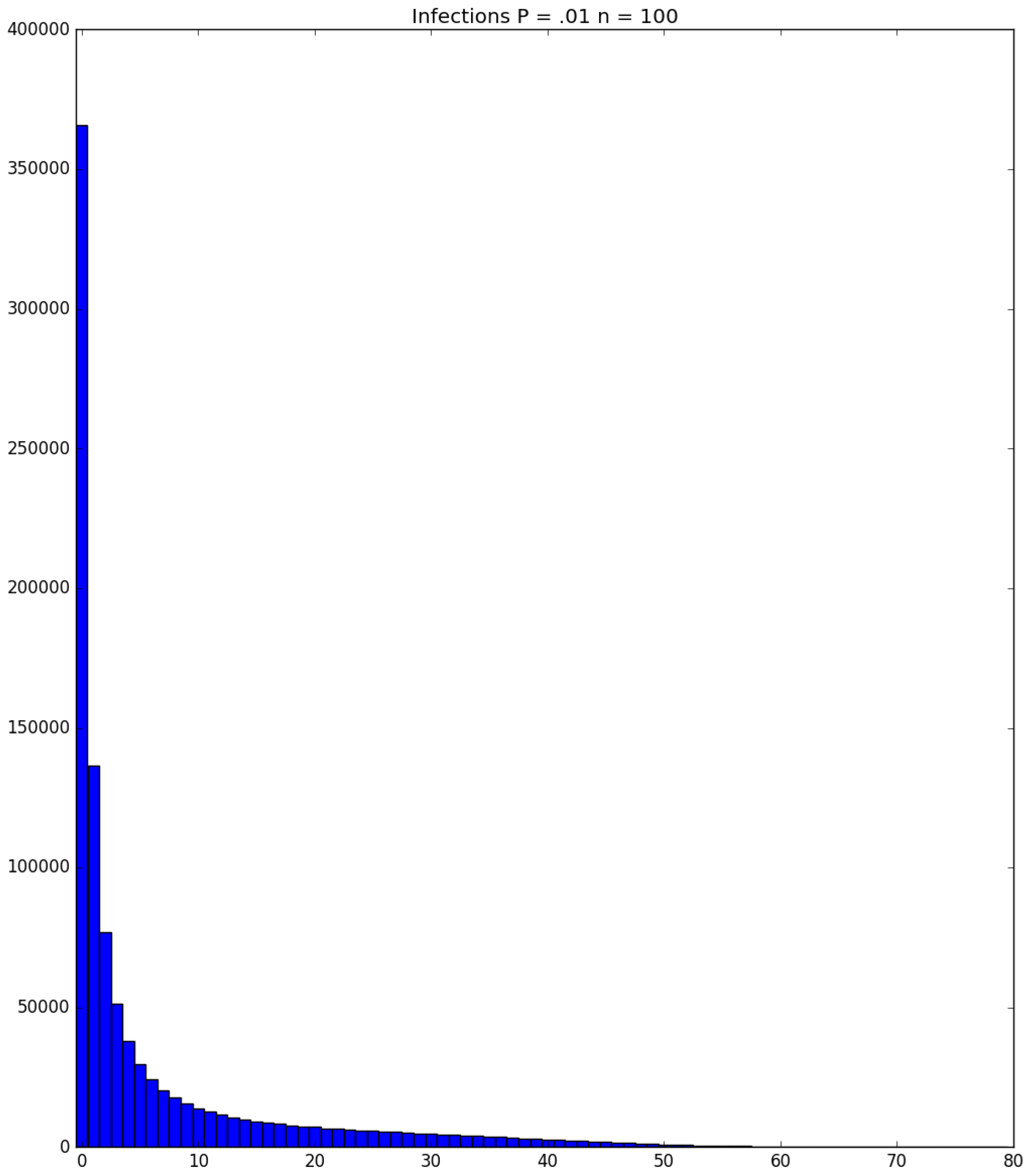
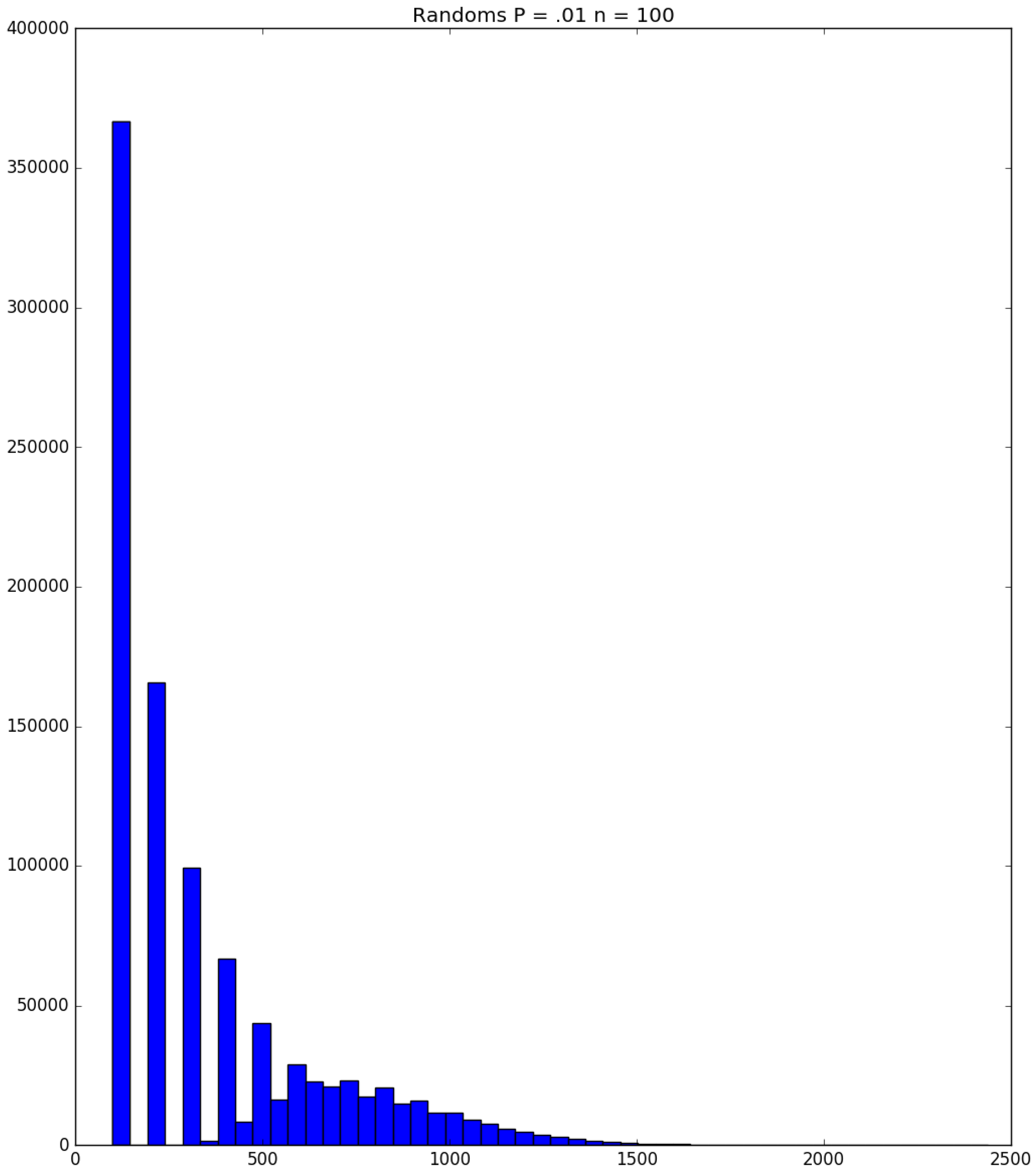
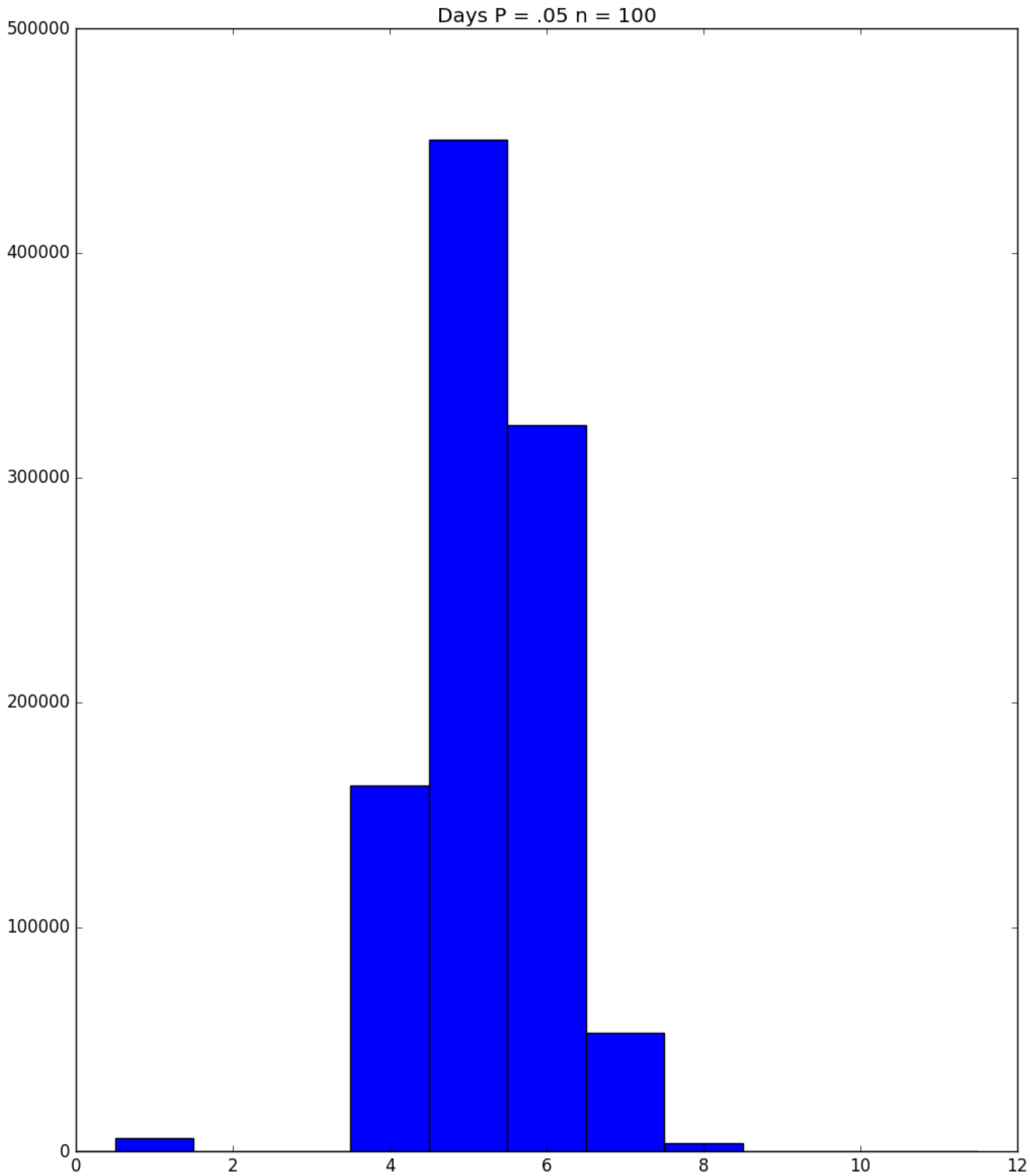
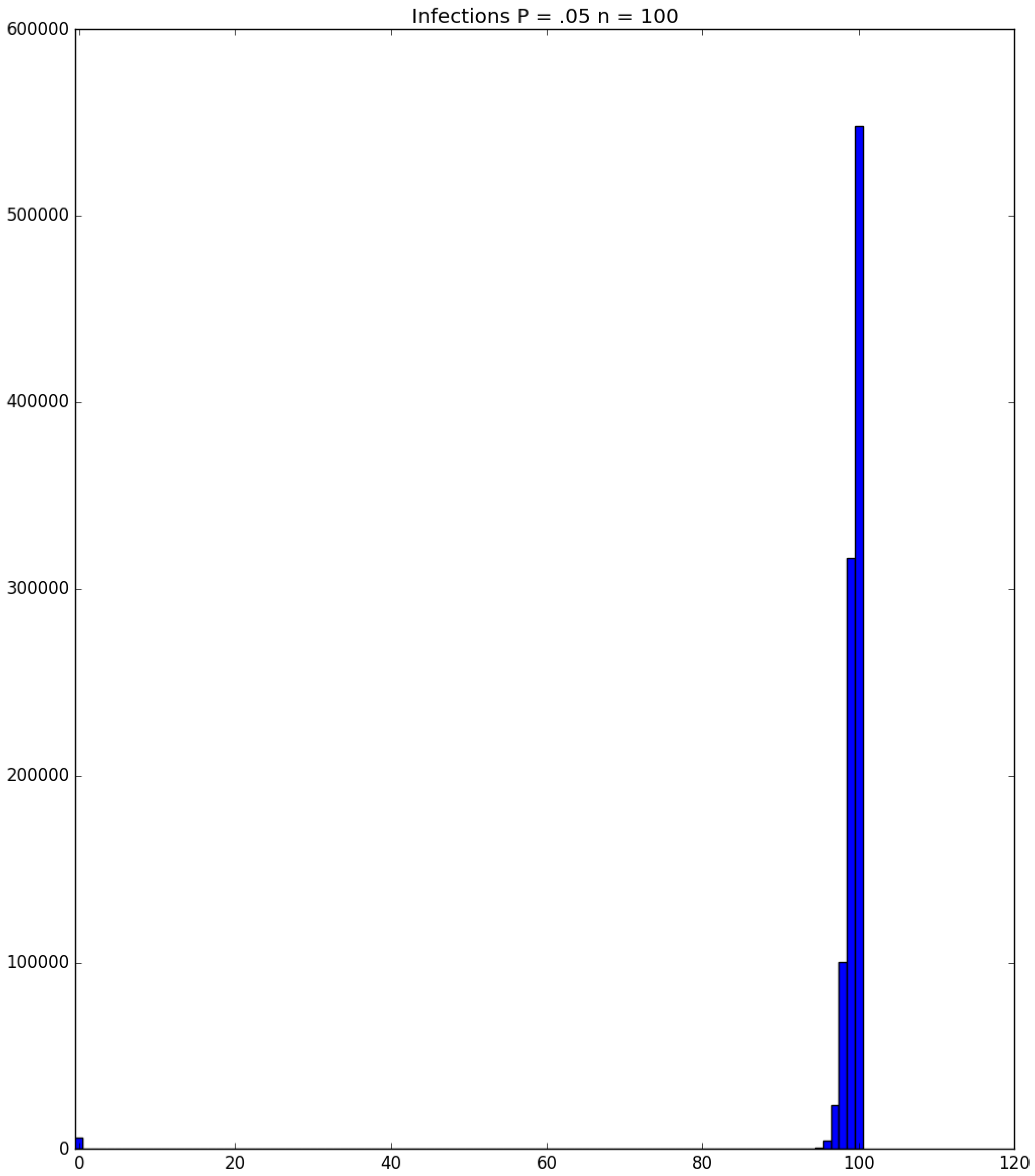
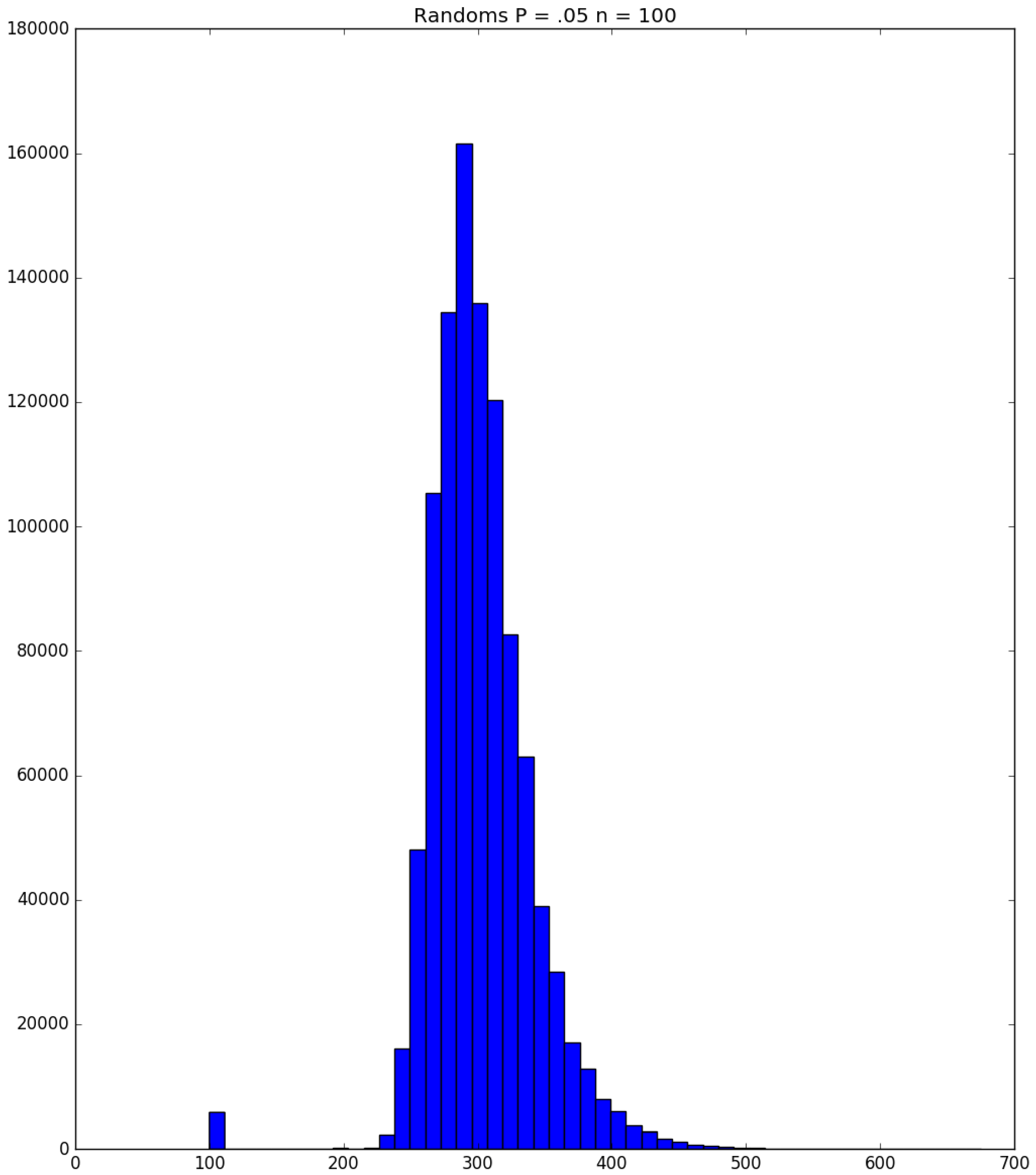
Example 3. Suppose that susceptibles are in a facility, and all are exposed to one infective on Day 1; the probability that a susceptible becomes infected upon exposure to an infective is ; and each infective stays infectious for exactly one day. Figure 5, Figure 6 and Figure 7 respectively depict histograms of the length of the pandemic (in days), the total number of individuals who eventually become infected (out of 100), and the number of PRNs used in the simulation. These histograms are based on 1,000,000 independent replications of the simulated pandemic. Figure 8, Figure 9 and Figure 10 depict the same outcome measures as the previous three, except that this latter set of figures is for the case . By design, replication i of the runs used many of the same green PRNs as replication i of the runs, . Figure 5 shows that, for small , the sample probability mass function (p.m.f.) of the length of the pandemic dies off quickly. It is actually possible for the pandemic to end after only one day—with probability —but the sample mean of the length of the pandemic is with a sample standard deviation of . Figure 6 reveals a similar p.m.f. for the number of individuals who become infected; here and , with the large standard deviation owing to a long right-hand tail. Figure 7 illustrates an interesting p.m.f. for the number B of PRNs (Bernoulli trials) used in the course of the simulations. That p.m.f. is characterized by distinct chunks of PRNs corresponding to the first few days of the pandemic; and we find that and . Figure 8 shows that, for the much higher , the p.m.f. of D is less variable, owing to the fact that the disease propagates throughout the population quite quickly, so that and . Figure 9 reveals that almost everyone eventually becomes infected, with and . Figure 10 illustrates a much tighter p.m.f. for the number of PRNs used in the case (compared to the case in Figure 7); here, we have and . □
3.3. Run Time and Efficiency Considerations
The pandemic simulation effort requires more than simply generating Bernoulli trials. One also has to make decisions, update statistcs, and access saved observations from temporary storage. How do these miscellaneous tasks affect the overall computation time with respect to green simulation? In this section, we present a number of results on the efficacy of our green simulation technology. Namely, Example 4 discusses simulation run-time savings on a more-realistic mixing example that what we have seen so far, and Example 5 illustrates how we can use variance reduction methods to carry out sensitivity analysis.
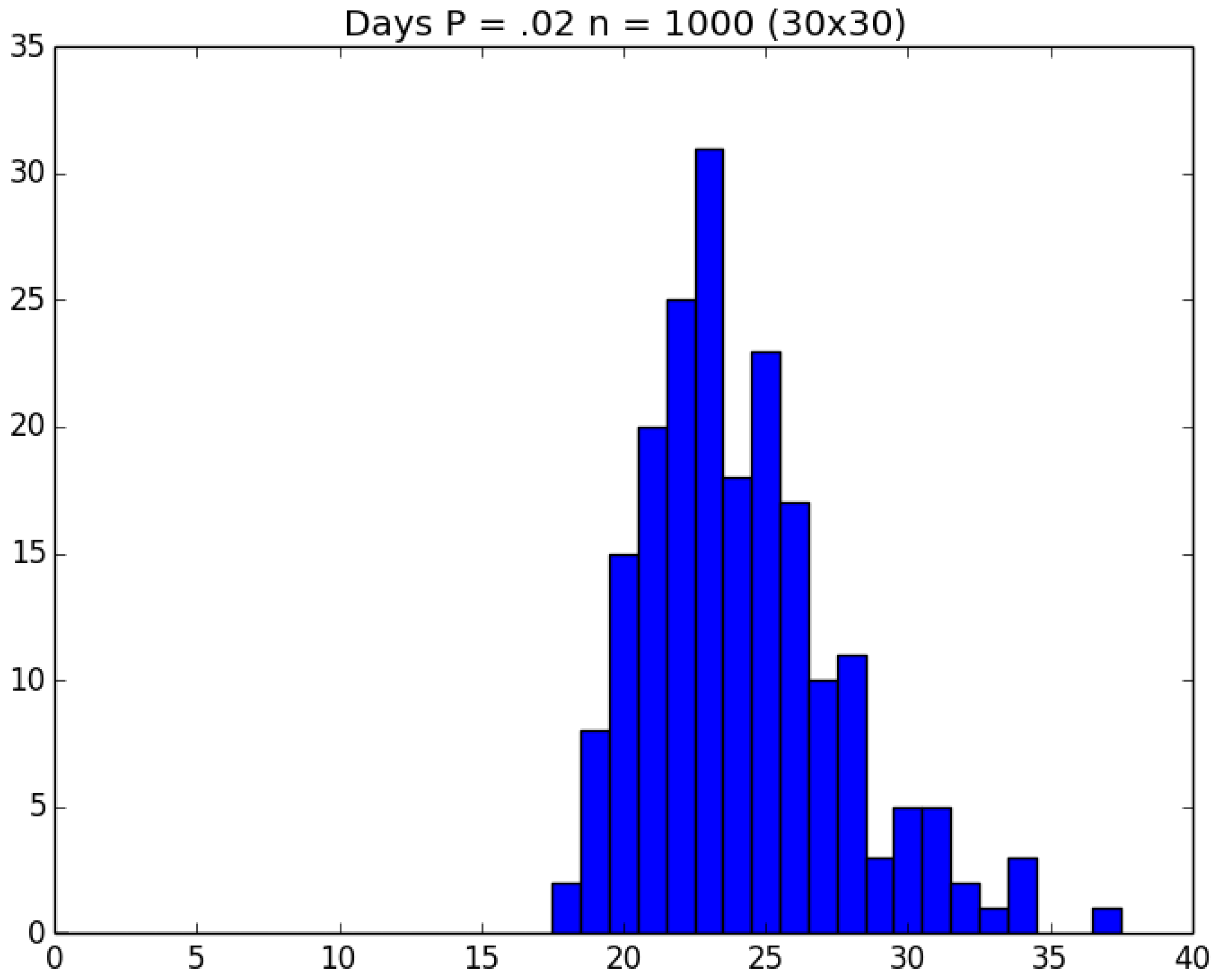
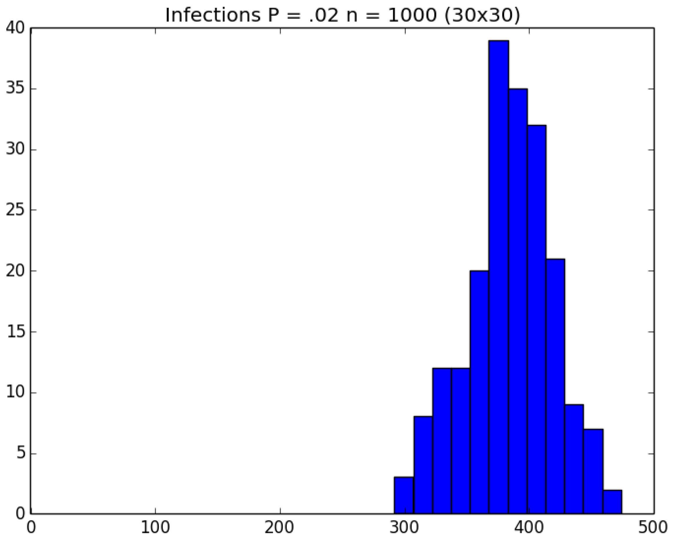
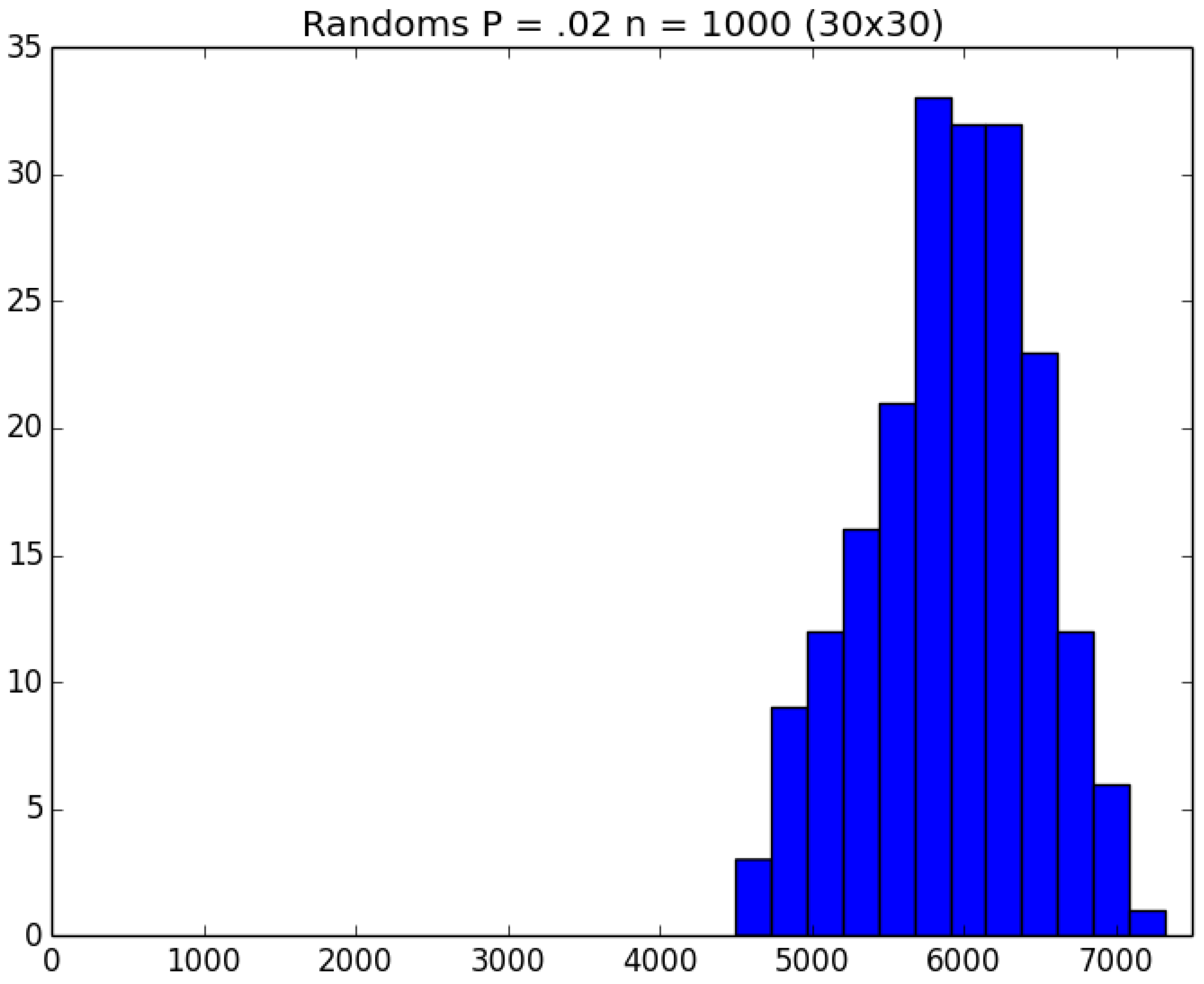
Example 4. Clock-Time Savings. Consider a school with 900 students and 100 staff members. The students are divided into 30 classrooms, each with 30 students; and each student remains in his/her assigned classroom all day. Each of the 100 staff members are randomly assigned 10 classrooms to visit during the day (and will visit those same assigned classrooms every day). Thus, each student interacts with the other 29 kids in his/her classroom as well as with the staff members who visit the classroom each day; and each staff member interacts with the other 99 staff members as well as with the 300 students whom the staff member visits in his/her assigned 10 classrooms. On Day 1, all 1000 people in the cohort are susceptibles. Unfortunately, the school principal (person 0) is infectious and visits all 1000 susceptibles on Day 1, any of whom subsequently become infected with probability p. The principal is so sick that he does not return after Day 1. However, anyone who gets infected becomes infectious the next day and remains infectious for a total of three days. We ran 200 replications of both the traditional (naive) and green versions of the simulation for each of the five choices of .
To get an idea of what we are facing, Figure 11, Figure 12 and Figure 13, respectively, depict histograms for the length of the pandemic, number of infections that occur, and the number of PRNs required for the baseline scenario for this example. In any case, the traditional replications required about 118 min of real clock time on a standard Windows-based PC; and the corresponding 1000 green replications required about 103 min—i.e., a savings of about 15% over running the five sets of experiments individually. □
Example 5. Sensitivity and Variance Reduction. The fact that we incorporate many of the same PRNs between runs of the simulation that use different values for parameter p suggests that the outputs from the runs may be positively correlated. For instance, suppose that denotes the sample mean of the number of individuals infected during the course of the simulation when the baseline Bernoulli parameter is p. If so that and are presumably positively correlated, then is an unbiased estimator for the true mean difference and, notably,so that the estimator for the mean difference has a smaller variance than would be observed if the runs had been undertaken independently—a standard simulation variance reduction technique known as common random numbers (see Law [14]). As a bonus, we immediately obtain an estimator for the derivative in the vicinity of ,Such derivatives are useful for sensitivity analysis, and are especially so if they are of reduced variance. To illustrate this approach, suppose we simulate each of two scenarios and , both involving individuals, one initial infective, and a one-day infectiousness period. We simulated both of the scenarios with three sets of 100,000 replications to examine the variability of the outcomes under two sampling schemes: The two scenarios are carried out independently (Case A), and the scenarios are carried out in green fashion (Case B). Table 5 shows that the differences produced by the green simulations have less variability than those produced by Case A. □


