Anomaly Detection Based on Mining Six Local Data Features and BP Neural Network

Abstract

Key performance indicators (KPIs) are time series with the format of (timestamp, value). The accuracy of KPIs anomaly detection is far beyond our initial expectations sometimes. The reasons include the unbalanced distribution between the normal data and the anomalies as well as the existence of many different types of the KPIs data curves. In this paper, we propose a new anomaly detection model based on mining six local data features as the input of back-propagation (BP) neural network. By means of vectorization description on a normalized dataset innovatively, the local geometric characteristics of one time series curve could be well described in a precise mathematical way. Differing from some traditional statistics data characteristics describing the entire variation situation of one sequence, the six mined local data features give a subtle insight of local dynamics by describing the local monotonicity, the local convexity/concavity, the local inflection property and peaks distribution of one KPI time series. In order to demonstrate the validity of the proposed model, we applied our method on 14 classical KPIs time series datasets. Numerical results show that the new given scheme achieves an average F₁-score over 90%. Comparison results show that the proposed model detects the anomaly more precisely.

1. Introduction

Key performance indicators (KPIs) are time series with the format of (timestamp, value), which can be collected from network traces, syslogs, web access logs, SNMP, and other data sources [1].

Table 1. Description of 14 classical KPIs.

	KPI1	KPI2	KPI3	KPI4	KPI5	KPI6	KPI7
Description	Periodic series	Periodic and fluctuation	Unstable series	Unstable series	Stable series	Unstable series	Unstable series
	KPI8	KPI9	KPI10	KPI11	KPI12	KPI13	KPI14
Description	Stable series	Unstable series	Continuous fluctuation series	Unstable series	Periodic and fluctuation series	Stable series	Continuous fluctuation series

shows the description of 14 classical KPIs and Figure 1 shows these 14 classical KPIs, which can be downloaded at http://iops.ai/dataset_list/. For example, KPI1 is a typical periodic data series [2], which is very common in our daily life. KPI5 is a classical stable data series [3], which may indicate the enterprise production index of one company. KPI11 is an unstable data series [4], in which the distribution of anomalies is very irregular. KPI10 and KPI14 belong to continuous fluctuation data series [5], of which the variation degree is dramatic so that anomalies could be detected very arduously. Furthermore, in KPI2, KPI3, KPI6, KPI8, and KPI12, the distribution between the normal data and the anomalies is extraordinarily unbalanced, which also results in the low accuracy of KPIs anomaly detection.

Anomaly detection is purposed to find “the variation”, as the so-called anomaly, from the norm KPI dataset. In recent years, anomaly detection plays an increasingly important role in some big data analysis areas. For example, in the field of finance, anomaly detection technology is used to detect fraud [6] and network intrusion in network security [7].

Up to now, many anomaly detection approaches have been proposed. In [8], Hu et al. proposed an anomaly detection method known as Robust SVM (RSVM). By neglecting noisy data and using averaging technique, the RSVM makes the decision surface smoother and controls regularization automatically. In [9], Kabir et al. proposed a Least Square SVM (LS-SVM) method. Compared with the standard SVM, this method behaves more sensitive to anomalous and noise in training set. By using an optimum allocation scheme and selecting samples depending on variability, the algorithm is optimized to produce an effective result. Since Bayesian Network can be used for an event classification scheme, it can also be used for anomaly detection. In [10], Kruegel et al. identified two reasons for a large amount of false alarms. The first reason is the simplistic aggregation of model outputs, which leads to high false positives. The second is that anomaly detection system may misjudge some unusual but legitimate behaviors. To solve these problems, an anomaly detection approach based on Bayesian Network was proposed in [10]. Neutral network is also applicable for detecting anomaly. In [11], Hawkins et al. presented a Replicator Neural Network (RNN). By providing an outlyingness factor for anomaly, the method reproduces the input data pattern at output layer after training and achieves high accuracy without class labels. For the statistics-based approaches, Shyu et al. proposed an effective method based on robust principal component analysis in [12]. The method was developed from two principal components. One of the principal components explains about half of the total variation, while the other minor component’s eigenvalues are less than 0.2. This technique has benefits of reducing dimension of data without losing important information and having low computational complexity.

One of the essential keys to develop anomaly detection models to detect the KPIs anomalies efficiently is time-series feature mining technique, which may affect the superior limit of the models. In previous studies, sliding window-based strategy was widely used for time series analysis, see for example [13,14,15,16] and the references therein. However, the prediction performance of this method relies on the description of similarity metrics between two sub-sequences. Moreover, in this method, similarity metrics are just represented by the calculation of the distance. In order to avoid the problem, Hu et al. proposed a meta-feature-based approach in [17], in which six statistics data characteristics including kurtosis, coefficient of variation, oscillation, regularity, square waves, and trend are mined. Nevertheless, these six statistics data characteristics are the features only representing the entire variation of the sequence described, and the relationship between several adjacent points are not revealed subtly (in other words, local variation situation between a few adjacent points could not be well described). We take the following coefficient of variation as an example, which describes the degree of dispersion of one time series

$$C=\frac{\sigma }{\mu },$$

(1)

where $C$ denotes the coefficient of variation of one time series, $\sigma$ denotes the standard deviation of this series, and $\mu$ is the mean value of this series. From Equation (1), we know that the coefficient of variation reflects the variation situation from an overall perspective of one time sequence, and thus the local variation situation could not be well reflected.

In the field of anomaly detection, generally, many anomalous events may have not happened successively or the probability of occurrence in succession is very small, which means one anomalous event usually appears suddenly and rarely. Therefore, due to the low frequency of abnormal events [18], we are not able to confirm an anomaly just using some characters describing the entire variation situation of one sequence, and we could not locate or predict the coming time of the next unknown anomaly precisely. In this situation, the subtle insight of local dynamics of the described sequence is particularly needed.

The major innovations of this work could be summarized as follows: we mine six local data features on behalf of the real-time dynamics of described time series. By means of vectorization description between every four adjacent points, the local geometric characteristics of one time series curve could be well described in a precise mathematical way. For example, local monotonicity, local convexity/concavity, and local inflection properties could be well revealed. Then input these six local data features into supervised back-propagation (BP) neural network, a new anomaly detection scheme is proposed. Numerical examples on the above 14 typical KPIs show that, taking advantage of the six local features as the inputs of the BP neural network, the new given scheme achieves an average F₁-score over 90%. Compared with the traditional statistics data characteristics used in [19], our method has a higher score, which means that our six local data features can be well described in the local dynamics of one KPI time series. Compared with SVM method [20] and SVM + PCA [21] method, our method based on BP neural network also has a higher average F₁-score.

The rest of this paper is organized as follows. Section 2 gives the basic concept of BP neural network. Besides, analysis of six local geometric characteristics is discussed in detail. Several numerical examples are given in Section 3 to argue the validity of our model. Discussion is given in the Section 4, and conclusion is summarized in Section 5.

2. Materials and Methods

Figure 2a shows the framework of our anomaly detection method. Figure 2b is the semantic drawing of six local data features spaces. By means of vectorization description on a normalized training/verifying dataset innovatively, the local geometric characteristics of one time series curve could be well described in a precise mathematical way. Thus six local data features have been mined to describe the local monotonicity, convexity/concavity, and the local inflection properties of one KPI series curve. Then input these six features into BP neural network, after multiple training processes, a new anomaly detection model is established.

2.1. BP Neural Network Method

In this subsection, we shall give a few necessary backgrounds on back-propagation (BP) neural network. We will merely mention a few mathematical statements necessary for a good understanding for the present paper, and more details can be found in [22,23,24,25,26].

BP neural network is a kind of artificial neural networks on the basis of error back-propagation algorithm. Usually, BP neural network consists of one input layer, one or more hidden layer, and one output layer.

Let m, k, respectively, denote the neural number of input layer and the neural number of output layer, and L denotes the number of hidden layers. Additionally, $Label=\left(l_1,l_2,\cdots ,l_k\right)$ denotes the target vector, $value=\left(v_1,v_2,\cdots ,v_m\right)$ denotes the input vector of BP neural network, $a^L=\left(a_1^L,a_2^L,\cdots a_k^L\right)$ denotes the output vector of BP. BP uses $f_l(x)$ as the neuron activation function in the lth layer, $l=1,2,\dots ,L$. The 1st layer of the neural network is input layer, from the 2nd layer to the $(L-1)\mathrm{th}$ layer are hidden layers, and layer Lth is the output layer. Let $w_{ij}^l$ denotes the weight from node i of layer (l − 1)th to node j of layer lth, and $b_j^l$ denotes the bias of node j in layer lth.

In BP neural network, the neurons just in adjacent layers are fully connected; nevertheless, there is no connection in the same neurons’ layer. After each training process, the output value (the vector of predicted labels) is compared with the target value (the vector of correct labels), and then we can amend weights and thresholds of the input layer and the hidden layer with error feedback. With a hidden layer, BP neural network can express any continuous function accurately.

Let $a_j^l$ denotes the output of node j in layer lth, and let $z_j^l$ denotes the assemble of inputs in node j of layer lth, and it can be expressed as follows [23]

$$z_j^l={\displaystyle \sum _k{w}_{kj}^l{a}_k^{l-1}}+b_j^l.$$

(2)

Therefore, the output $a_j^l$ of node $j$ in layer lth is expressed as follows

$$a_j^l=f_l(z_j^l)=f_l({\displaystyle \sum _k{w}_{kj}^l{a}_k^{l-1}}+b_j^l),$$

(3)

where $f_l(x)$ is the activation function of layer lth.

There are three transfer functions in the BP neural network such that tan-sigmod, log-sigmoid, and purelin. Tan-sigmod or purelin transfer function maps any input value into an output value between −1 and 1. Log-sigmoid transfer function maps any input value into an output value between 0 and 1. The transfer functions in neural network can mix freely without unifying, so that we can reduce the network’s parameters and hidden layer’s nodes during the establishment of BP.

Since $Label$ is the target vector, and $a^L$ is output vector, the error function $E\left(w,b\right)$ can be expressed as follows [23]

$$E\left(w,b\right)={\Vert Label-a^L\Vert }^2={\displaystyle \sum _{i=1}^k{\left(l_i-y_i\right)}^2},$$

(4)

where k denotes the number of output layer nodes.

In this paper, we use the following mean square error (MSE) as the error output function of BP neural network [23]

$$MSE=\frac{1}{2p}{\displaystyle \sum _{n=1}^p{\Vert Label({\mathrm{x}}_n)-a^L(x_n)\Vert }^2},$$

(5)

where $x_n$ denotes the input of each train sample, and $P$ denotes the number of train samples. It can decrease the global error of training dataset and the local error when each data point inputs.

In order to reduce the MSE gradually so that the predicted output value can be closer and closer to expectations booked in advance, BP neural network needs to adjust its weights and bias values constantly [24].

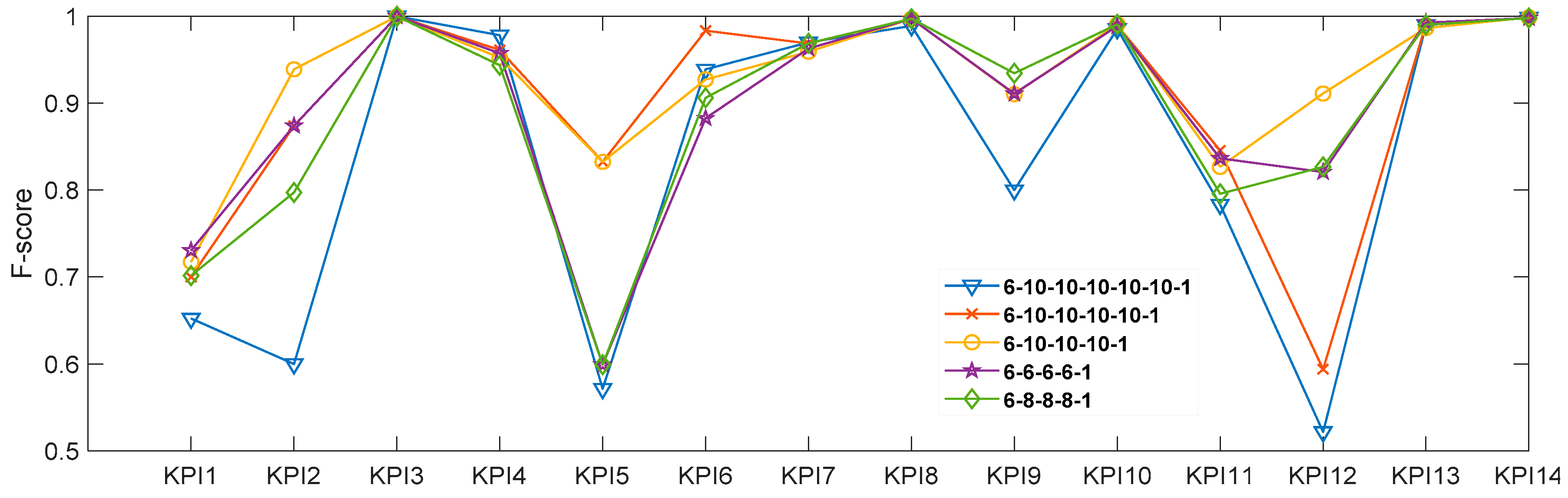
The classification accuracy of BP neural network is heavily dependent on the selected topology and on the selection of the training algorithm [25]. In this paper, we use Widrow-Hoff LMS method [26] to adjust the weight $w_{ij}^l$ and bias $b_j^l$, that is

$$w_{ij}^l=w_{ij}^l-\eta \left(\frac{\partial MSE}{\partial w_{ij}^l}\right),$$

(6)

$$b_j^l=b_j^l-\eta \left(\frac{\partial MSE}{\partial b_j^l}\right),$$

(7)

where $\eta$ is used to control its amendment speed, which can be variable or constant, generally speaking $0<\eta <1$.

According to the basic principle of BP neural network, we can obtain the update formula of weight and bias in each layer.

We write ${\delta }_j^L$ for the value of $\partial MSE/\partial z_j^L$, which can be expressed as follows

$${\delta }_j^L=\frac{\partial MSE}{\partial z_j^L}=\frac{\partial MSE}{\partial a_j^L}\frac{\partial a_j^L}{\partial z_j^L}=\frac{\partial MSE}{\partial a_j^L}{f}_L^{\prime }(z_j^L),$$

(8)

where $f^{\prime }$ of the formula above is the first-order partial derivatives of the activation function of layer lth $f_l(x)$.

And we write ${\delta }_j^l$ for the value of $\partial MSE/\partial z_j^l$, which can be expressed as follows

$${\delta }_j^l=\frac{\partial MSE}{\partial z_j^l}={\displaystyle \sum _k\frac{\partial MSE}{\partial z_k^{l+1}}\frac{\partial z_k^{l+1}}{\partial z_j^l}}={\displaystyle \sum _k\frac{\partial z_k^{l+1}}{\partial z_j^l}{\delta }_k^{l+1}},$$

(9)

since

$$z_k^{l+1}={\displaystyle \sum _i{w}_{ik}^{l+1}{a}_i^l}+b_k^{l+1}={\displaystyle \sum _i{w}_{ik}^{l+1}{f}_l(z_i^l)}+b_k^{l+1},$$

(10)

we have $\partial z_k^{l+1}/\partial z_j^l=w_{jk}^{l+1}{f^{\prime }}_l(z_j^l)$, then ${\delta }_j^l$ can be defined by recurrence as follows:

$${\delta }_j^l={\displaystyle \sum _k{w}_{jk}^{l+1}{f}_l^{\prime }(z_j^l){\delta }_k^{l+1}}.$$

(11)

Similarly, we can prove that [23]

$$\frac{\partial MSE}{\partial b_j^l}=\frac{\partial MSE}{\partial z_j^l}\frac{\partial z_j^l}{\partial b_j^l}={\delta }_j^l,$$

(12)

$$\frac{\partial MSE}{\partial w_{kj}^l}=\frac{\partial MSE}{\partial z_j^l}\frac{\partial z_j^l}{\partial w_{kj}^l}=a_k^{l-1}{\delta }_j^l=f_{l-1}(z_k^{l-1}){\delta }_j^l.$$

(13)

Consequently, the basic idea of BP neural network is summarized as follows. Firstly, input training data into neural network. Then during the processing of continuous learning and training, BP neural network will modify the weights and threshold values step by step, and when it reaches the precision error setup in advance, it will stop the learning. Finally, the output value is acquired.

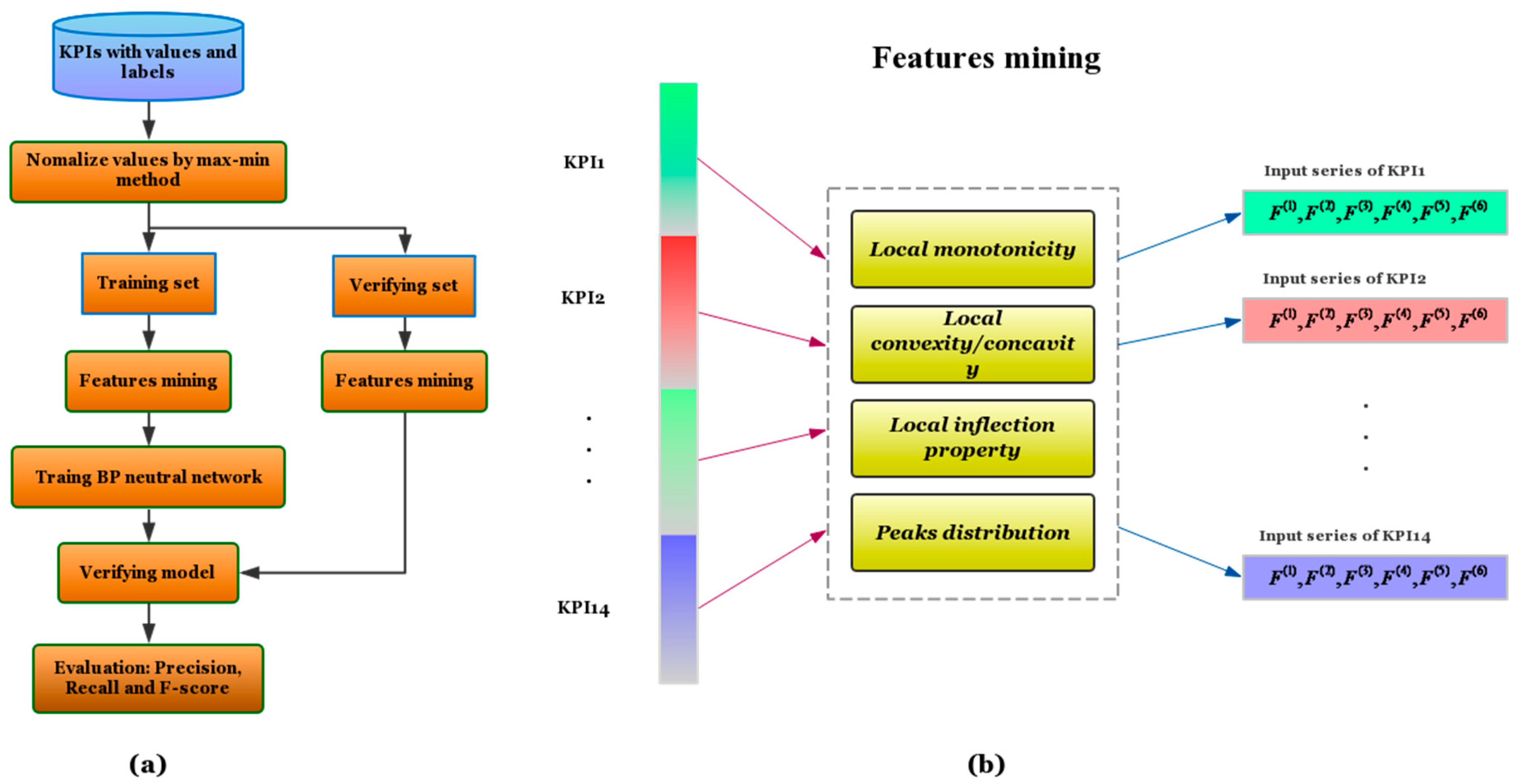
2.2. Features Mining Method

By means of vectorization description on a normalized KPIs dataset innovatively, the local geometric characteristics of one time series curve could be well described in a precise mathematical way. We shall mine six local data features to describe the local monotonicity, convexity/concavity, the local inflection properties of one series curve.

2.2.1. Normalization by Max–Min Method

For a KPIs data with value set $V=\left\{V_1,V_2,V_3,\cdots V_n,\cdots V_{n+m}\right\}$, we firstly use a max–min method to normalize each of the values as follows:

$$v_i=\frac{V_i-V_{\min }}{V_{\max }-V_{\min }},$$

(14)

where $V_{\max }=\underset{i}{\max }{V}_i,V_{\min }=\underset{i}{\min }{V}_i,i=1,2,\dots ,n+m.$ The purpose of normalization is to avoid large differences between different values in a KPI time series.

2.2.2. The Definition of Six Local Data Features

For a resulting normalized value dataset $v=\left\{v_1,v_2,v_3,\cdots v_n,\cdots v_{n+m}\right\}$, we divide it into a train part $V_{train}=\left\{v_1,v_2,v_3,\cdots v_n\right\}$ and a verifying or test part $V_{test}=\left\{v_{n+1},v_{n+2},v_{n+3},\cdots v_{n+m}\right\}$. We shall use the train part to establish the model while use the verifying part to test the performance of the model.

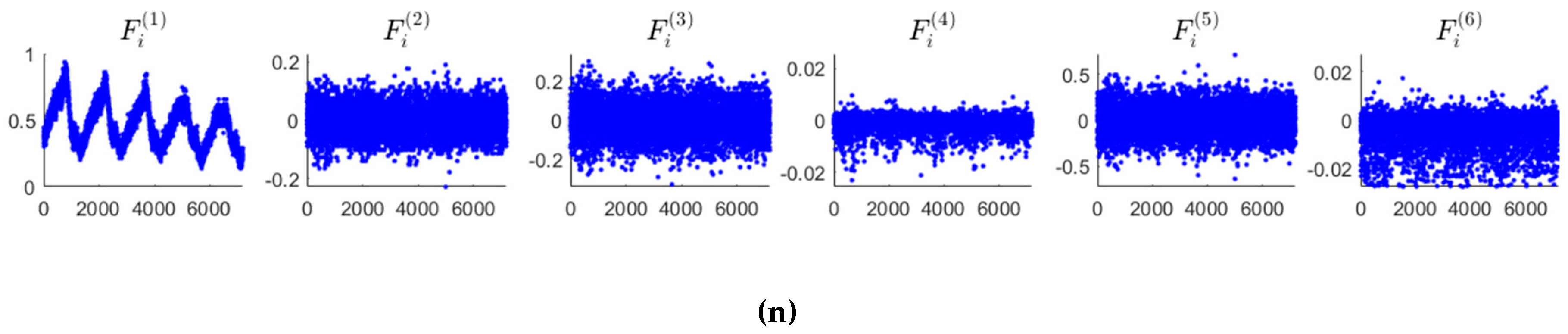
Local monotonicity, convexity/concavity, local inflection properties, and peaks distribution are four essential features of a given data set, which describe the local increasing/decreasing rates of the data set. With this in mind, we mine the following six features of the resulting normalized value dataset $v=\left\{v_1,v_2,v_3,\cdots v_n,\cdots v_{n+m}\right\}$

$$\{\begin{array}{l}{F}_i^{(1)}=v_i,\hspace{1em}i=1,2,\dots ,n+m,\\ F_i^{(2)}=v_{i+1}-v_i,\hspace{1em}i=1,\dots ,n+m-1,\\ F_i^{(3)}=v_{i+2}-2v_{i+1}+v_i,\hspace{1em}i=1,2,\dots ,n+m-2,\\ F_i^{(4)}=\left(v_{i+2}-v_{i+1}\right)\left(v_{i+1}-v_i\right),\hspace{1em}i=1,2,\dots ,n+m-2,\\ F_i^{(5)}=v_{i+3}-3v_{i+2}+3v_{i+1}-v_i,\hspace{1em}i=1,2,\dots ,n+m-3,\\ F_i^{(6)}=\left(v_{i+3}-2v_{i+2}+v_{i+1}\right)\left(v_{i+2}-2v_{i+1}+v_i\right),\hspace{1em}i=1,2,\dots ,n+m-3.\end{array}$$

(15)

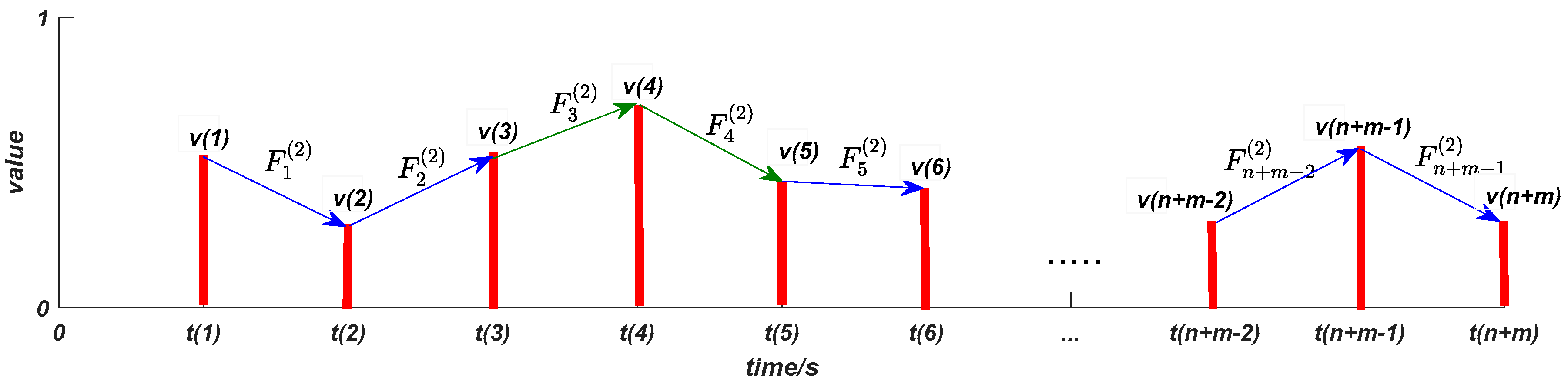
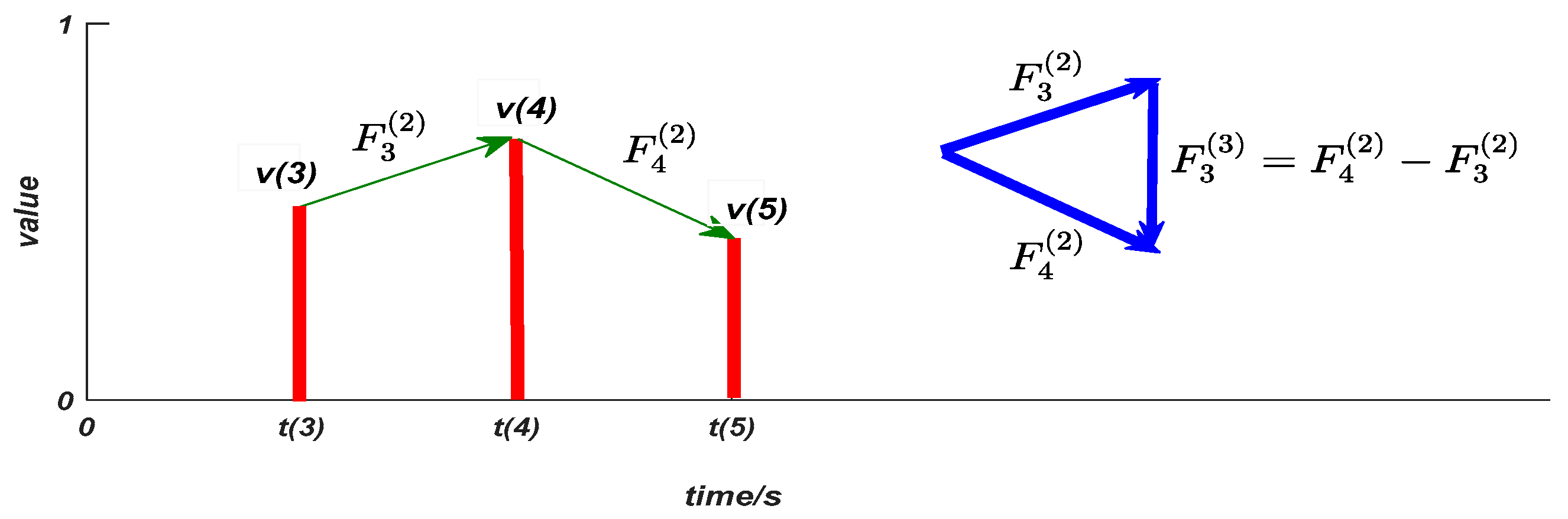
We give some geometric explanations on the six mined features. The feature $F_i^{(1)}$ can describe peaks distribution of the normalized value data. As shown in Figure 3 and Figure 4, the feature $F_i^{(2)}$ and $F_i^{(3)}$ are in fact the first and second difference of the normalized value data, respectively, which can describe the local monotonicity and convexity/concavity of the normalized value data. For example, with $F_i^{(2)}>0,F_{i+1}^{(2)}>0$ and $F_i^{(3)}>0$, the normalized value data is both monotonically increasing and convex locally (in other words, the normalized value data has a faster and faster increasing rate locally).

The feature $F_i^{(4)}$ can describe the local inflection property of the normalized value data. For example, with $F_i^{(4)}<0,$ that is $F_i^{(2)}>0,F_{i+1}^{(2)}<0$ or $F_i^{(2)}<0,F_{i+1}^{(2)}>0$, it implies that the normalized value data has a local switch between “increasing” and “decreasing” values. The feature $F_i^{(5)}$ is the third difference of the normalized value data, and the feature $F_i^{(6)}$ can describe the local switch of the sign of $F_i^{(4)}$.

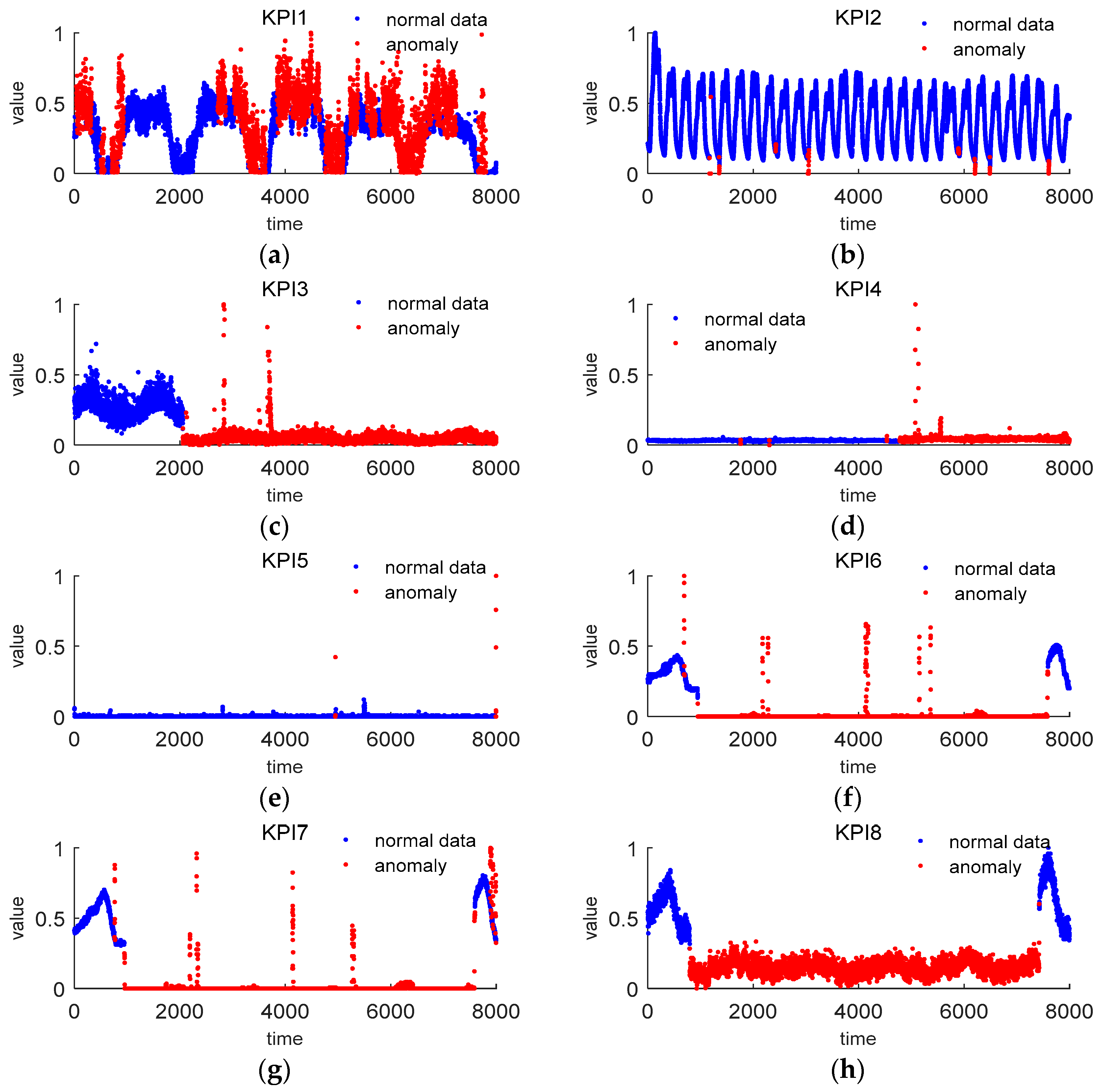
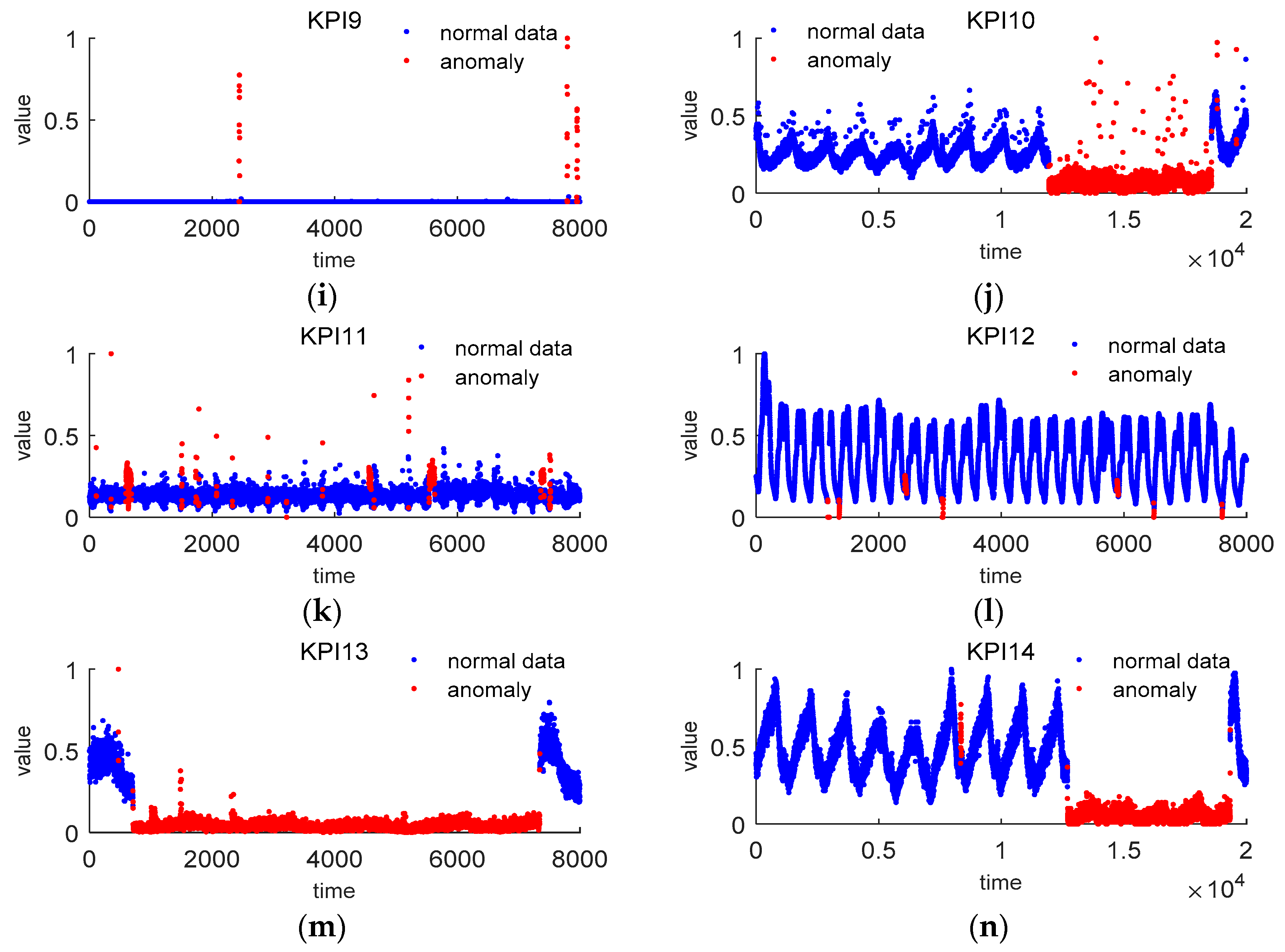
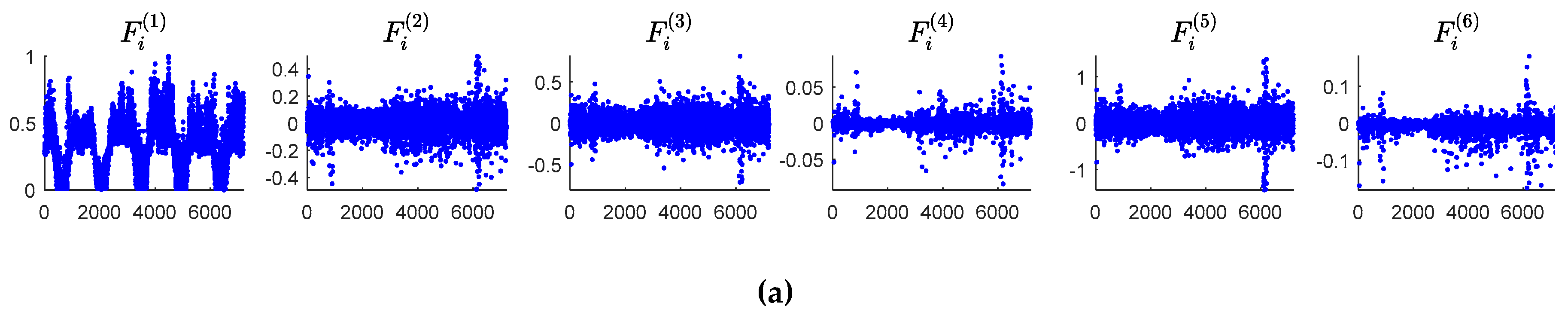
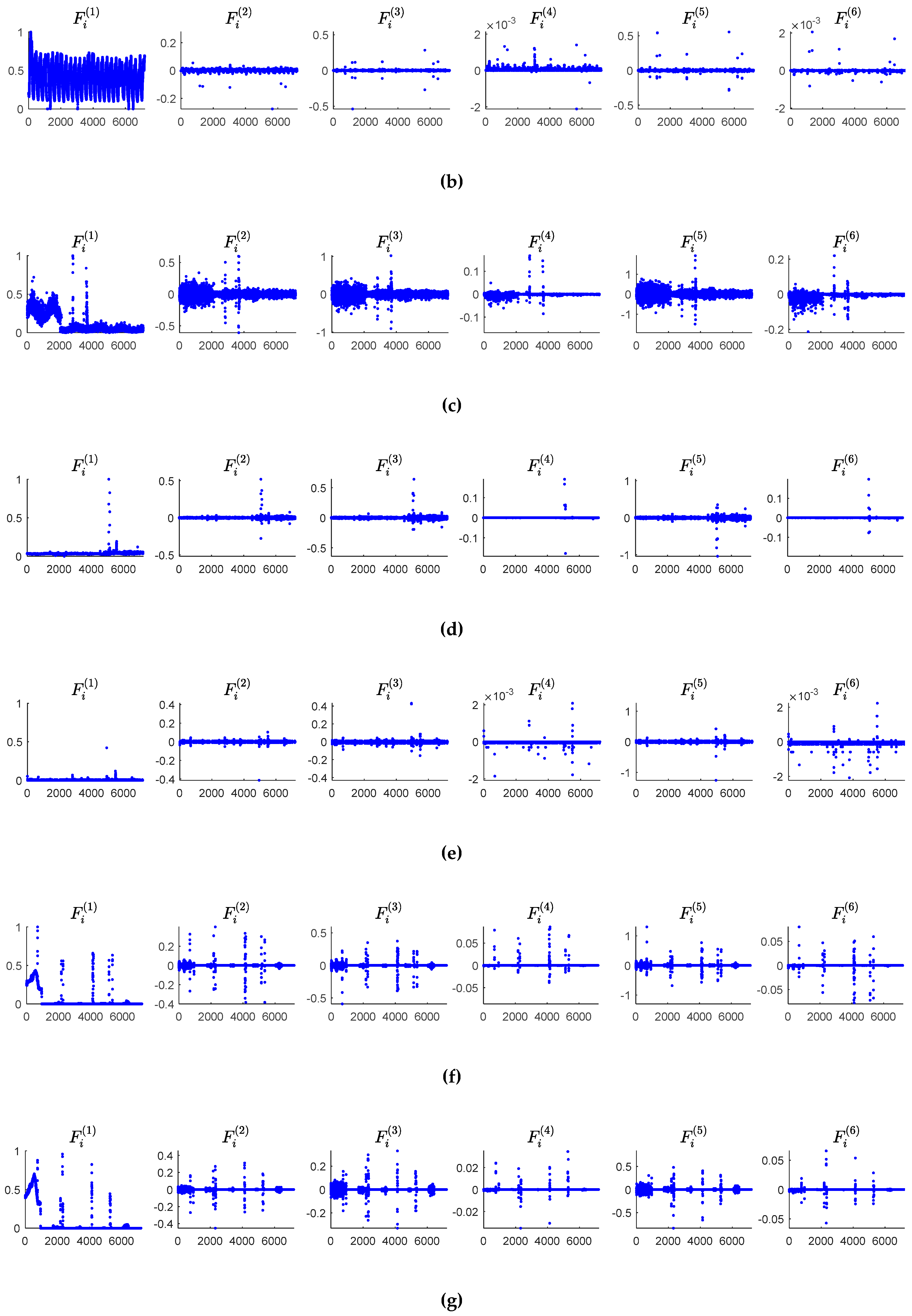
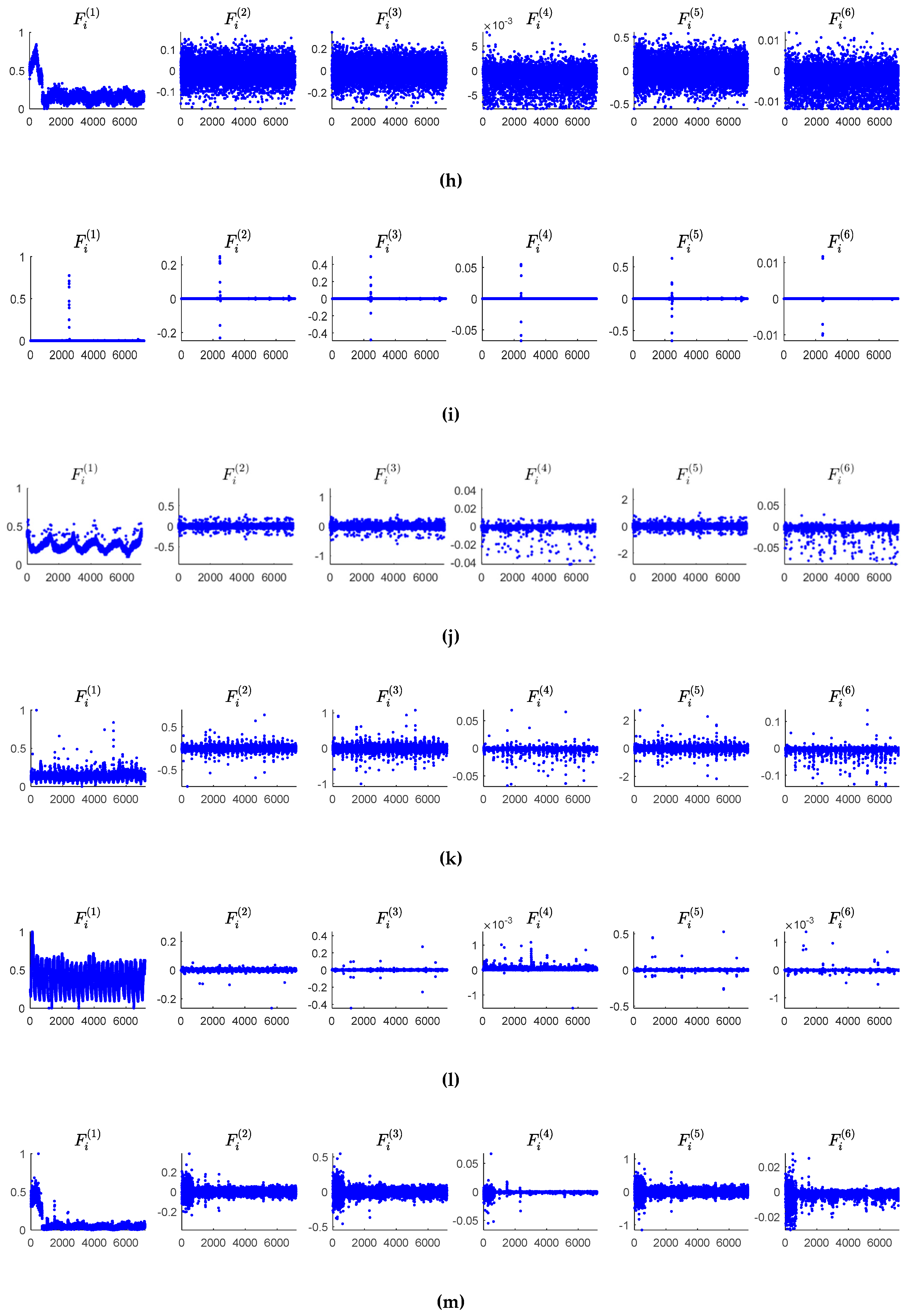
Figure 5 shows the numerical results of the six features mined of 14 KPIs. From this figure, we can see that the first, second, and third difference $F_i^{(2)},F_i^{(3)}$ and $F_i^{(5)}$ distinguish anomalies and normal data significantly. The point whose values of $F_i^{(2)},F_i^{(3)}$ and $F_i^{(5)}$ differ from that of the other points extraordinarily may be considered as an anomaly. The features $F_i^{(4)}$ and $F_i^{(6)}$ reveal the anomalies in a subtle way, which can prevent the misjudgments given by $F_i^{(2)},F_i^{(3)}$, and $F_i^{(5)}$.

2.3. Algorithm Description

Input:

In training model, we input

$$\begin{array}{l}{F}^{(1)}=\left\{F_4^{(1)},F_5^{(1)},\cdots F_n^{(1)}\right\},\\ F^{(2)}=\left\{F_3^{(2)},F_4^{(2)},\cdots F_{n-1}^{(2)}\right\},\\ F^{(3)}=\left\{F_2^{(3)},F_3^{(3)},\cdots F_{n-2}^{(3)}\right\},\\ F^{(4)}=\left\{F_2^{(4)},F_3^{(4)},\cdots F_{n-2}^{(4)}\right\},\\ F^{(5)}=\left\{F_1^{(5)},F_2^{(5)},\cdots F_{n-3}^{(5)}\right\},\\ F^{(6)}=\left\{F_1^{(6)},F_2^{(6)},\cdots F_{n-3}^{(6)}\right\}.\end{array}$$

In verifying model, we input

$$\begin{array}{l}{F}^{(1)}=\left\{F_{n+1}^{(1)},F_{n+2}^{(1)},\cdots F_{n+m}^{(1)}\right\},\\ F^{(2)}=\left\{F_n^{(2)},F_{n+1}^{(2)},\cdots F_{n+m-1}^{(2)}\right\},\\ F^{(3)}=\left\{F_{n-1}^{(3)},F_n^{(3)},\cdots F_{n+m-2}^{(3)}\right\},\\ F^{(4)}=\left\{F_{n-1}^{(4)},F_n^{(4)},\cdots F_{n+m-2}^{(4)}\right\},\\ F^{(5)}=\left\{F_{n-2}^{(5)},F_{n-1}^{(5)},\cdots F_{n+m-3}^{(5)}\right\},\\ F^{(6)}=\left\{F_{n-2}^{(6)},F_{n-1}^{(6)},\cdots F_{n+m-3}^{(6)}\right\}.\end{array}$$

Output:

The output is the predicted label vector;

• Step 1: normalize the values of KPIs series data;
• Step 2: separate the KPI into training dataset and verifying dataset;
• Step 3: calculate the value of six local data features according to Equations (14) and (15);
• Step 4: input features vector and target vector into BP algorithm;
• Step 5: BP neural network outputs the detecting results.

2.4. Evaluation Method of Model Performance

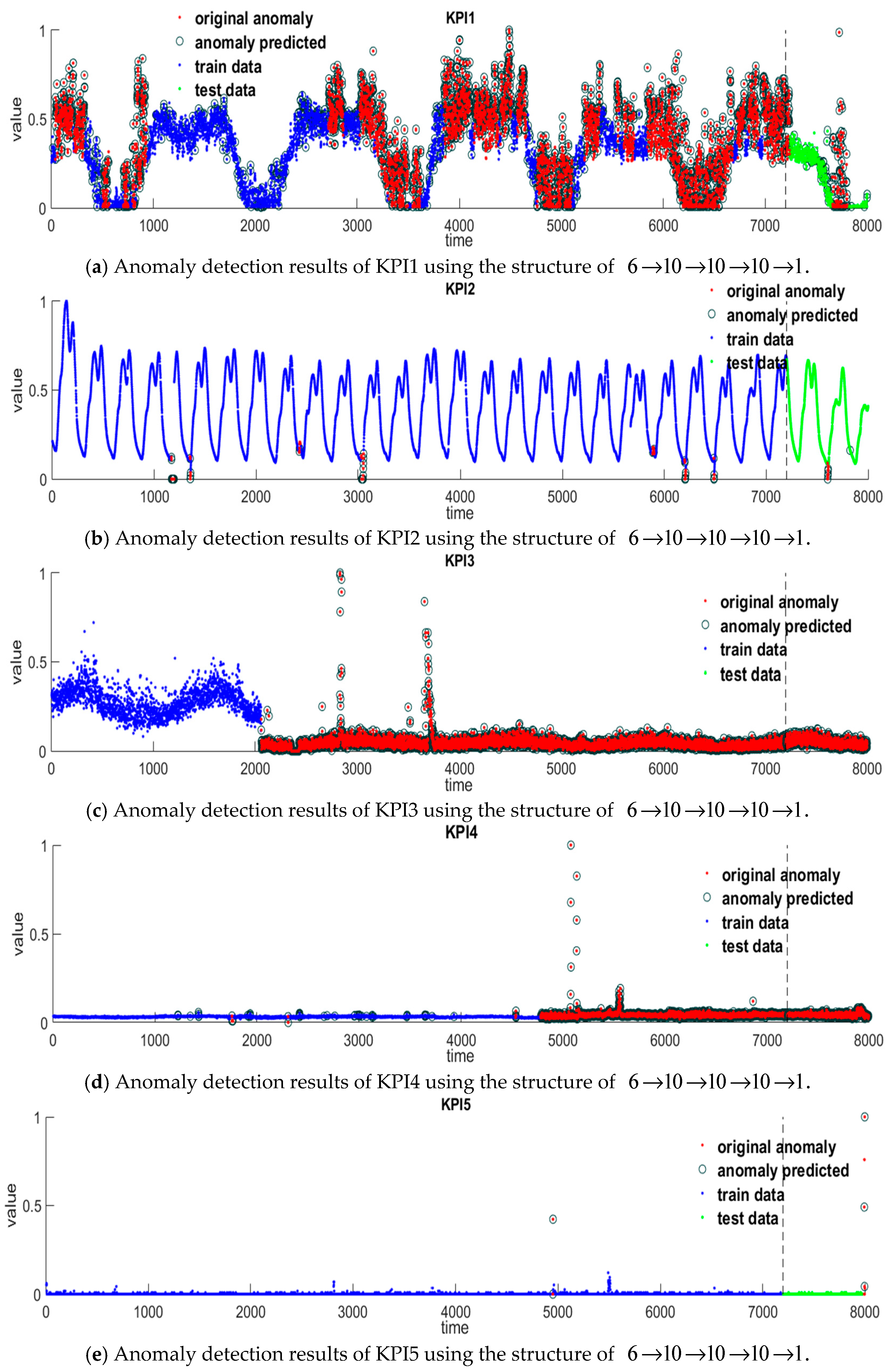
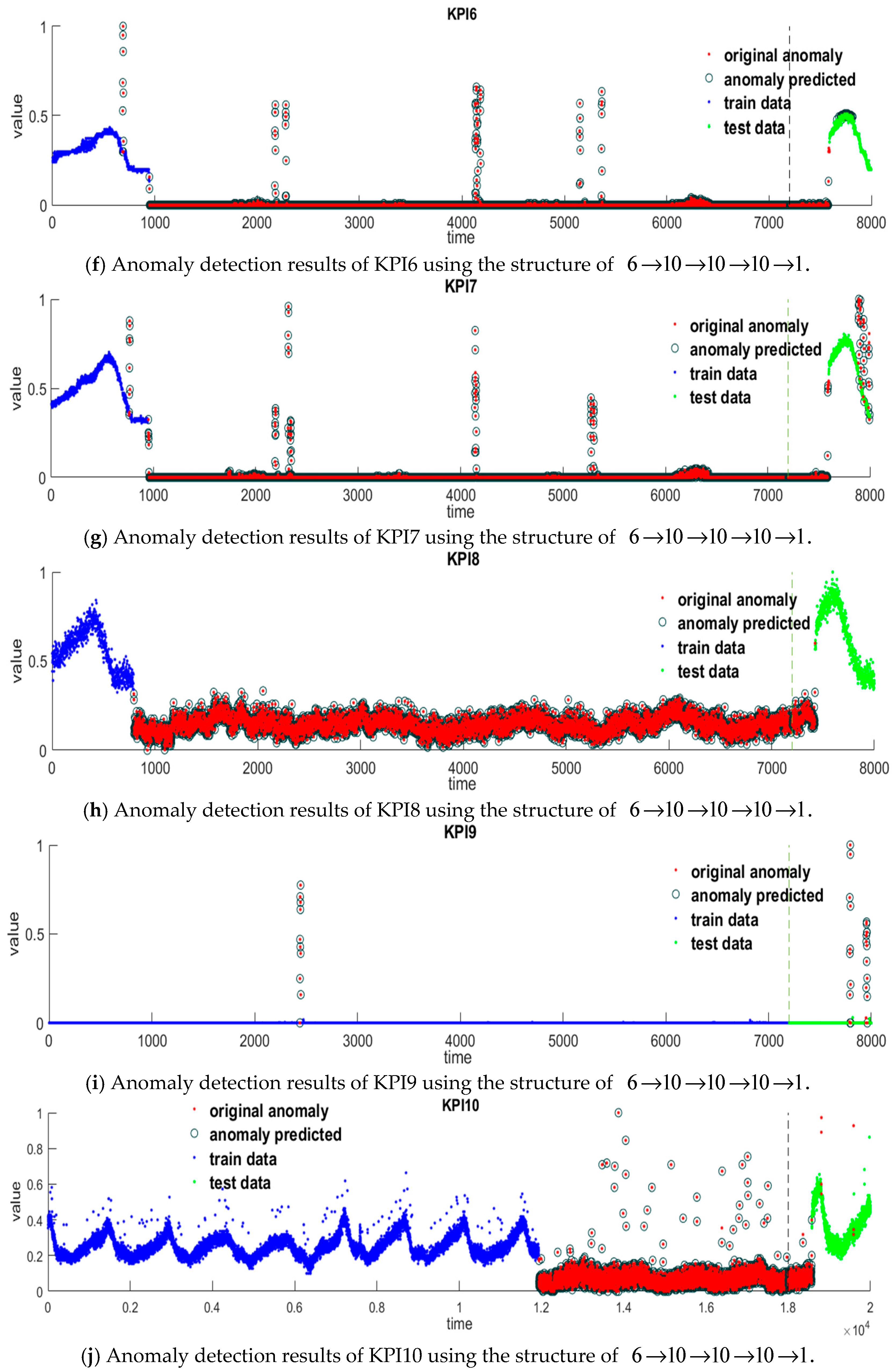
In this experiment, confusion matrices (TP, TN, FP, and FN) have been applied to define the evaluation criterion. The meaning corresponding to confusion matrices are categorized in

Table 2. The meaning of confusion matrices.

	Actual Value
Predication Value		Anomaly	Normal
	Anomaly	TP	FP
	Normal	FN	TN

, where true positive (TP) means the number of anomalies precisely diagnosed as anomalies, whereas true negative (TN) means the number of normal data correctly diagnosed as normal. In the same way, false positive (FP) means the number of normal data diagnosed as anomalous by mistake, and false negative (FN) means the number of anomalies inaccurately diagnosed as normal.

In order to give the evaluations of the performance of the proposed model, evaluation criteria such as Recall, Precision, and F₁-score are considered [18]

$$Recall=\frac{TP}{TP+FN},$$

(16)

$$Precision=\frac{TP}{TP+FP},$$

(17)

$$F_{1-}score=2\times \frac{Precision\times Recall}{Precision+Recall}.$$

(18)

Recall, which is computed by Equation (16), denotes the number of anomalies detected by the anomaly detection technology. Precision, which is computed by Equation (17), denotes the numbers of the values being accurately categorized as anomalies. It is the most intuitive performance evaluation criterion. F₁-score, which is computed by Equation (18), consists of a harmonic mean of precision and recall while accuracy is the ratio of correct predictions of a classification model [27,28]. In the next numerical experiments, we shall adopt the F₁-score to evaluate the performance of the model.

3. Results

In next experiments, we shall use the computer with 8 GB memory as well as core i5 inside. The model is established by MATLAB 2016a.

3.1. Explore Different Topology Structures of BP Network

Inputting six mined local data features into BP neural network, a novel anomaly detection model is proposed. In order to find out the best-performing topology structure of BP network, we have done five experiments to explore the optimal combination of different layers and neural nodes. Figure 6 shows the F₁-scores of different topology structures of BP network for each of 14 KPIs.

Table 3. Comparative results of different topology structures of back-propagation (BP) network.

	6 → 6 → 6 → 6 → 1	6 → 8 → 8 → 8 → 1	6 → 10 → 10 → 10 → 1	6 → 10 → 10 → 10 → 10 → 1	6 → 10 → 10 → 10 → 10 → 10 → 1
${Precision|}_{average}$ (%)	96.50	96.59	96.80	97.68	94.76
${Recall|}_{average}$ (%)	85.58	84.41	89.33	85.64	88.64
${F_1-score|}_{average}$ (%)	89.66	88.93	92.92	90.33	91.60

shows the average score of different topology structures of BP network. From these, we can see that the topology structure of $6\to 10\to 10\to 10\to 1$ has the highest average F₁-score among the five topology structures. The topology structure of $6\to 10\to 10\to 10\to 1$ means 6 input nodes, 10 nodes of each hidden layer, and 1 output node. We use the log-sigmoid function as the transfer function in the BP neural network. It should be noted that when the predicted label is no smaller than 0.5, it will be set as 1, otherwise 0. In other words, a data point with the predicted label above 0.5 is regarded as an anomaly while under 0.5 is regarded as a normal data. In the next compared experiments, we shall use the best structure of $6\to 10\to 10\to 10\to 1$ to establish the BP model.

3.2. Results Presentation

We show the numerical results of the structure of $6\to 10\to 10\to 10\to 1$ on each of 14 KPIs.

Table 4. Values of evaluation criteria using our method.

	KPI1	KPI2	KPI3	KPI4	KPI5	KPI6	KPI7	KPI8	KPI9	KPI10	KPI11	KPI12	KPI13	KPI14
Precision (%)	86.25	99.50	100	95.25	99.75	88.25	94.87	99.88	99.38	99.55	97.38	97.25	98.00	99.90
Recall (%)	61.41	88.89	100	95.25	71.43	97.69	97.00	99.55	84.00	98.62	71.83	85.71	99.32	99.85
F1-score (%)	71.74	93.90	100	95.25	83.25	92.73	95.92	99.71	91.04	99.08	82.67	91.12	98.65	99.88

shows the values of three evaluation criteria of the verifying dataset of each of 14 KPIs. From the results, we can see that the detection effects on these 14 KPIs are good, especially for KPI 3. All the anomalies had been detected and there is no misjudgments happened in KPI 3. According to Equation (19), the new given scheme achieves an average F₁-score over 90%, which verifies the remarkable anomaly detection effects.

$${F_1-score|}_{average}=2\times \frac{{Precision|}_{average}\times {Recall|}_{average}}{{Precision|}_{average}+{Recall|}_{average}}=92.92\%.$$

(19)

Figure 7 shows the numerical results of the structure of $6\to 10\to 10\to 10\to 1$ on each of 14 KPIs. In the figure, the red points are original anomalies of one KPI. The circles represent the predicted anomalies. When the circle coincides in position with one red point, it means that this abnormal data point has been detected by our method. From Figure 7, we know that on the left of the dotted line, the detection results of the train models achieve a higher accuracy, while there are a few misjudgments taking place in this process. On the right of the dotted line, the detection results about verifying data are shown. For KPI1, which is a periodic time series, our method is not capable to achieve satisfactory performance. There are some anomalies that have not been detected and some normal data are misjudged as anomalies. For KPI2–KPI10, numerical results show a remarkable detection effect. For KPI11, although there are some anomalies that have not been detected, misjudgments are rare, which means that once a point is diagnosed as an anomaly, this point may well be an original anomaly. For KPI12–KPI14, numerical results also show a remarkable detection effect.

4. Discussion

In this section, firstly, we use the traditional statistics data features given in [19] as the input of BP network, and apply this model on the same KPIs. Secondly, we also explore SVM [20] and SVM + PCA [21] methods and the results are presented as well. Finally, we analyze the performance of these models.

4.1. Traditional Statistics Data Features and BP Network

We performed an experiment using the traditional statistics data features given in [19] and BP network with topology structure of $6\to 10\to 10\to 10\to 1$. These traditional statistics data features included average value, maximum value, minimum value, standard deviation, and variance of one time series. The results are presented in

Table 5. Values of evaluation criteria using the method in [19].

	KPI1	KPI2	KPI3	KPI4	KPI5	KPI6	KPI7	KPI8	KPI9	KPI10	KPI11	KPI12	KPI13	KPI14
Precision (%)	66.12	54.55	100	100	50.00	90.57	97.90	100	90.0	98.29	95.92	37.50	99.33	99.93
Recall (%)	64.36	66.67	100	95.75	66.67	97.46	96.11	97.80	72.0	98.80	66.20	85.71	98.67	99.78
F1-score (%)	65.23	60.00	100	97.83	57.14	93.89	97.00	98.89	80.0	98.55	78.33	52.17	99.00	99.85

. According to Equations (16)–(18), we have

$${Precision|}_{average}=84.29\%,{Recall|}_{average}=86.14\%,{F_1-score|}_{average}=85.20\%.$$

4.2. Explore Different Machine Learning Models

In this subsection, we shall use SVM [20] and SVM + PCA [21] methods to further verify the validity of the six new mined features given in Equation (15).

● SVM method

Table 6. Values of evaluation criteria using SVM method.

	KPI1	KPI2	KPI3	KPI4	KPI5	KPI6	KPI7	KPI8	KPI9	KPI10	KPI11	KPI12	KPI13	KPI14
Precision (%)	69.94	0	100	100	100	97.96	96.80	100	100	100	100	96.00	100	100
Recall (%)	61.96	0	100	95.50	14.29	98.46	97.69	99.55	84.00	98.27	70.42	100	98.63	98.73
F1-score (%)	65.71	NaN	100	97.70	25.00	98.21	97.24	99.78	91.30	99.13	82.64	97.96	99.31	99.36

shows the anomaly detection results using SVM method with the six new mined features given in Equation (15) as the input. From the results, it is observed that SVM-based method is not able to find any anomaly in KPI2, but it has a high score on the other KPIs. The average score on the other 13 KPIs are calculated as follows:

$${Precision|}_{average}=96.98\%,{Recall|}_{average}=85.93\%,{F_1-score|}_{average}=91.12\%.$$

● SVM + PCA Method

Table 7. Values of evaluation criteria using SVM + PCA method.

	KPI1	KPI2	KPI3	KPI4	KPI5	KPI6	KPI7	KPI8	KPI9	KPI10	KPI11	KPI12	KPI13	KPI14
Precision (%)	46.91	100	100	100	100	74.03	85.60	99.55	100	100	100	100	100	100
Recall (%)	61.96	66.67	99.88	92.50	14.28	97.95	96.07	99.55	80.00	98.10	67.61	42.86	98.63	97.53
F1-score (%)	53.40	80.00	99.94	96.10	25.00	84.33	90.53	99.55	88.89	99.04	80.67	60.00	98.63	98.75

shows the anomaly detection results using SVM + PCA method with the six new mined features given in Equation (15) as the input. The detection results for the combined SVM and PCA methods have some improvements. However, as for KPI5, this method shows a poor performance. The average score has been calculated as follows:

$${Precision|}_{average}=93.29\%,{Recall|}_{average}=79.54\%,{F-score|}_{average}=85.87\%.$$

4.3. Performance Analysis of Different Models

Table 8. Comparative results of different methods.

	Our Method	Method in Literature [19]	SVM Method	SVM + PCA Method
${Precision|}_{average}$(%)	96.80	84.29	96.98	93.29
${Recall|}_{average}$(%)	89.33	86.14	85.93	79.54
${F_1-score|}_{average}$(%)	92.92	85.20	91.12	85.87

shows the comparative results on the same 14 KPIs using different methods. Our method, SVM method, and SVM + PCA method all use the six new mined features given in Equation (15) as the input. And our method is established by using BP network with the structure of $6\to 10\to 10\to 10\to 1$. Besides, the method in [19] is also established by using BP network with the same structure, which the traditional statistics data characteristics are inputted into. As can be seen from Table 8, compared with the traditional statistics data characteristics used in [19], our method has a higher score, which means that our six local data features can well describe the local dynamics of the KPIs. Compared with SVM and SVM + PCA methods, our method also has a higher score, which means that BP network has a better anomaly detection effect. In the whole, our method is capable for anomaly detection on some complexity KPIs.

5. Conclusions

We have proposed six local data features to mine the local monotonicity, the local convexity/concavity, the local inflection properties, and peaks distribution of KPI time series data. With these six local data features as the input of BP network, we have established a new anomaly detection model.

Compared with the traditional statistics data characteristics method given in [19], our scheme shows a higher accuracy and universality which demonstrates the remarkable detection effects. Our experiments also show that BP neural network has a better universality and accuracy degree than SVM and SVM + PCA methods. In the future, some other neural network algorithms will be explored to further this study. In addition, the classification accuracy of BP neural network is heavily dependent on the selected topology and on the selection of the training algorithm, and the performance of our proposed methodology could be further improved by selecting more sophisticated training algorithms in the future work.

Since our method is based on mining six local data features, as for periodic data series like KPI1, these local data features are not adequate enough to characterize the periodic data series. In the future study, we shall mine some features describing the periodic time series.

References

1. Pérez-Álvarez, J.M.; Maté, A.; Gómez-López, M.T.; Trujillob, J. Tactical Business-Process-Decision Support based on KPIs Monitoring and Validation. Comput. Ind. 2018, 102, 23–39. [Google Scholar] [CrossRef]
2. Yang, J.; Wan, W.; Yu, P.S. Mining Asynchronous Periodic Patterns in Time Series Data. IEEE Trans. Knowl. Data Eng. 2003, 15, 613–628. [Google Scholar] [CrossRef]
3. Kruczek, P.; Wyłomańska, A.; Teuerle, M.; Gajda, J. The modified Yule-Walker method for α-stable time series models. Phys. A Stat. Mech. Appl. 2017, 469, 588–603. [Google Scholar] [CrossRef]
4. Grillenzoni, C. Forecasting unstable and nonstationary time series. Int. J. Forecast. 1998, 14, 469–482. [Google Scholar] [CrossRef]
5. Pierini, J.; Telesca, L. Fluctuation analysis of monthly rainfall time series. Fluct. Noise Lett. 2010, 20, 219–228. [Google Scholar] [CrossRef]
6. Ahmed, M.; Mahmood, A.N.; Islam, M.R. A survey of anomaly detection techniques in financial domain. Future Gener. Comput. Syst. 2016, 55, 278–288. [Google Scholar] [CrossRef]
7. Hong, J.H.; Liu, C.C.; Govindarasu, M. Integrated Anomaly Detection for Cyber Security of the Substations. IEEE Trans. Smart Grid 2014, 5, 1643–1653. [Google Scholar] [CrossRef]
8. Hu, W.J.; Liao, Y.; Vemuri, V.R. Robust support vector machines for anomaly detection in computer security. In Proceedings of the International Conference Machine Learning & Applications-ICMLA, Los Angeles, CA, USA, 23–24 July 2003. [Google Scholar]
9. Kabir, E.; Hu, J.; Wang, H.; Zhuo, G. A novel statistical technique for intrusion detection systems. Future Gener. Comput. Syst. 2018, 79, 303–318. [Google Scholar] [CrossRef]
10. Kruegel, C.; Mutz, D.; Robertson, W.; Valeur, F. Bayesian event classification for intrusion detection. In Proceedings of the 19th Annual Computer Security Applications Conference, Las Vegas, NV, USA, 8–12 December 2003. [Google Scholar]
11. Hawkins, S.; He, H.; Williams, G.; Baxter, R. Outlier detection using replicator neural networks. In Data Warehousing and Knowledge Discovery, Proceedings of the International Conference on Data Warehousing and Knowledge Discovery, Aix-en-Provence, France, 4–6 September 2002; Lecture Notes in Computer Science; Kambayashi, Y., Winiwarter, W., Arikawa, M., Eds.; Springer: Berlin/Heidelberg, Germany, 2002; Volume 2454, pp. 170–180. [Google Scholar]
12. Shyu, M.L.; Chen, S.C.; Kanoksri, S.; Chang, L.W. A novel anomaly detection scheme based on principal component classifier. In IEEE Foundations and New Directions of Data Mining Workshop; Miami Univ Coral Gables Fl Dept of Electrical and Computer Engineering: Coral Gables, FL, USA, 2003; pp. 171–179. [Google Scholar]
13. Zhang, T.; Yue, D.; Gu, Y.; Wang, Y.; Yu, G. Adaptive correlation analysis in stream time series with sliding windows. Comput. Math. Appl. 2008, 57, 937–948. [Google Scholar] [CrossRef]
14. Ding, Z.; Fei, M. An anomaly detection approach based on isolation forest algorithm for streaming data using sliding window. IFAC Proc. 2013, 46, 12–17. [Google Scholar] [CrossRef]
15. Ren, H.; Ye, Z.; Li, Z. Anomaly detection based on a dynamic Markov model. Inf. Sci. 2017, 411, 52–65. [Google Scholar] [CrossRef]
16. Chou, J.S.; Ngo, N.T. Time series analytics using sliding window metaheuristic optimization-based machine learning system for identifying building energy consumption patterns. Appl. Energy 2016, 177, 751–770. [Google Scholar] [CrossRef]
17. Hu, M.; Ji, Z.W.; Yan, K.; Guo, Y.; Feng, X.W.; Gong, J.H.; Zhao, X. Detecting Anomalies in Time Series Data via a Meta-Feature Based Approach. IEEE Access 2018, 6, 27760–27776. [Google Scholar] [CrossRef]
18. Liu, D.; Zhao, Y.; Xu, H.; Sun, Y.; Pei, D.; Luo, J.; Jing, X.; Feng, M. Opprentice: Towards practical and automatic anomaly detection through machine learning. In Proceedings of the Internet Measurement Conference AMC, Tokyo, Japan, 28–30 October 2015. [Google Scholar]
19. Kumar, P.H.; Patil, S.B.; Sandya, H.B. Feature extraction, classification and forecasting of time series signal using fuzzy and garch techniques. In Proceedings of the National Conference on Challenges in Research & Technology in the Coming Decades National Conference on Challenges in Research & Technology in the Coming Decades (CRT 2013) IET, Ujire, India, 27–28 September 2013. [Google Scholar]
20. Amraee, S.; Vafaei, A.; Jamshidi, K.; Adibi, P. Abnormal event detection in crowded scenes using one-class SVM. Signal Image Video Proc. 2018, 12, 1115–1123. [Google Scholar] [CrossRef]
21. Li, Z.C.; Zhitang, L.; Bin, L. Anomaly detection system based on principal component analysis and support vector machine. Wuhan Univ. J. Nat. Sci. 2006, 11, 1769–1772. [Google Scholar]
22. Dong, X.F.; Lian, Y.; Liu, Y.J. Small and multi-peak nonlinear time series forecasting using a hybrid back propagation neural network. Inf. Sci. 2018, 424, 39–54. [Google Scholar] [CrossRef]
23. Maren, A.J.; Harston, C.T.; Pap, R.M. Handbook of Neural Computing Applications; Academic Press: San Diego, CA, USA, 1990. [Google Scholar]
24. Hagan, M.T.; Beale, M.H.; Demuth, H.B. Neural Network Design; PWS Pub: Boston, MA, USA, 1996. [Google Scholar]
25. Livieris, I. Improving the Classification Efficiency of an ANN Utilizing a New Training Methodology. Informatics 2018, 6, 1. [Google Scholar] [CrossRef]
26. Livieris, I.; Pintelas, P.E. A Survey on Algorithms for Training Artificial Neural Networks; Technical Report TR08-01; Department of Math, University of Patras: Patras, Greece, 2008. [Google Scholar]
27. Livieris, I.; Kiriakidou, N.; Kanavos, A.; Tampakas, V.; Pintelas, P. On Ensemble SSL Algorithms for Credit Scoring Problem. Informatics 2018, 5, 40. [Google Scholar] [CrossRef]
28. Powers, D. Evaluation: From Precision, Recall and F-Measure to ROC, Informedness, Markedness & Correlation. J. Mach. Learn. Technol. 2011, 2, 37–63. [Google Scholar]
Figure 1. Fourteen classical key performance indicators (KPIs). (a): Periodic time series; (b): Periodic and continuous fluctuation time series; (c): Unstable time series; (d): Unstable time series; (e): Stable time series; (f): Unstable time series; (g): Unstable time series; (h): Stable time series; (i): Unstable time series; (j): Continuous fluctuation time series; (k): Unstable time series; (l): Periodic and continuous fluctuation time series; (m): Stable time series; (n): Continuous fluctuation time series.
Symmetry 11 00571 g001aSymmetry 11 00571 g001b
Figure 2. (a): The flowchart of the proposed approach for KPIs time series; (b): the semantic drawing of six local data feature space.
Symmetry 11 00571 g002
Figure 3. Schematic illustration of the feature F i ( 2 ) .
Symmetry 11 00571 g003
Figure 4. Schematic illustration of the feature F i ( 2 ) and F i ( 3 ) .
Symmetry 11 00571 g004
Figure 5. Six features mined of the KPIs. (a) Six features mined of the KPI1; (b) Six features mined of the KPI2; (c) Six features mined of the KPI3; (d) Six features mined of the KPI4; (e) Six features mined of the KPI5; (f) Six features mined of the KPI6; (g) Six features mined of the KPI7; (h) Six features mined of the KPI8; (i) Six features mined of the KPI9; (j) Six features mined of the KPI10; (k) Six features mined of the KPI11; (l) Six features mined of the KPI112; (m) Six features mined of the KPI13; (n) Six features mined of the KPI14.
Symmetry 11 00571 g005aSymmetry 11 00571 g005bSymmetry 11 00571 g005cSymmetry 11 00571 g005d
Figure 6. F1-scores of different topology structures of BP network for each of 14 KPIs.
Symmetry 11 00571 g006
Figure 7. Anomaly detection results using the structure of 6 10 10 10 1 . (a): Anomaly detection results of KPI1 using the structure of 6 10 10 10 1 ; (b): Anomaly detection results of KPI2 using the structure of 6 10 10 10 1 ; (c): Anomaly detection results of KPI3 using the structure of 6 10 10 10 1 ; (d): Anomaly detection results of KPI4 using the structure of 6 10 10 10 1 ; (e): Anomaly detection results of KPI5 using the structure of 6 10 10 10 1 ; (f): Anomaly detection results of KPI6 using the structure of 6 10 10 10 1 ; (g): Anomaly detection results of KPI7 using the structure of 6 10 10 10 1 ; (h): Anomaly detection results of KPI8 using the structure of 6 10 10 10 1 ; (i): Anomaly detection results of KPI9 using the structure of 6 10 10 10 1 ; (j): Anomaly detection results of KPI10 using the structure of 6 10 10 10 1 ; (k): Anomaly detection results of KPI11 using the structure of 6 10 10 10 1 ; (l): Anomaly detection results of KPI12 using the structure of 6 10 10 10 1 ; (m): Anomaly detection results of KPI13 using the structure of 6 10 10 10 1 ; (n): Anomaly detection results of KPI14 using the structure of 6 10 10 10 1 .
Symmetry 11 00571 g007aSymmetry 11 00571 g007bSymmetry 11 00571 g007c