Parity-Assisted Generation of Nonclassical States of Light in Circuit Quantum Electrodynamics

Abstract

We propose a method to generate nonclassical states of light in multimode microwave cavities. Our approach considers two-photon processes that take place in a system composed of N extended cavities and an ultrastrongly coupled light–matter system. Under specific resonance conditions, our method generates, in a deterministic manner, product states of uncorrelated photon pairs, Bell states, and W states in different modes on the extended cavities. Furthermore, the numerical simulations show that the generation scheme exhibits a collective effect which decreases the generation time in the same proportion as the number of extended cavity increases. Moreover, the entanglement encoded in the photonic states can be transferred towards ancillary two-level systems to generate genuine multipartite entanglement. Finally, we discuss the feasibility of our proposal in circuit quantum electrodynamics. This proposal could be of interest in the context of quantum random number generator, due to the quadratic scaling of the output state.

1. Introduction

The state-of-the-art devices exhibiting quantum behaviour has grown extensively in the last two decades. Remarkable platforms such as superconducting circuits [1,2,3] and circuit quantum electrodynamics (QED) [4,5] have allowed the implementation of microwave quantum photonics [6,7], where superconducting electrical circuits mimic the behavior of atoms and cavities [8,9,10]. In this manner, the capability of tailoring internal circuit parameters to obtain devices with long coherence times and switchable coupling strengths yielded quantum optics experiments such as electromagnetically induced transparency [11], photon blockade [12], and lately to manipulate the parity symmetric of an artificial atom in situ [13] to name a few. A distinctive aspect of microwave photonics is the inherent nonlinearity coming from Josephson junction devices that makes possible to build photonic crystals with Kerr and Cross–Kerr nonlinearities much larger than the one observed in optical devices [14,15,16,17,18]. This allows for enhancing processes such as parametric down conversion [19,20,21,22], and the generation of nonclassical states of light [23,24,25,26,27]. Likewise, the notable features of superconducting circuits have also triggered a bunch of proposals for microwave photon generation in systems composed of a large number of cavities. In this context, it is possible to find proposals for the generation of entangled photon states such as NOON (MOON), corresponding to a photonic state where the resonator A has N (M) or zero quanta, entangled with resonator B with zero or N quanta [28,29,30,31,32] states, studies of correlated photons emitted from a cascade system [33], as well as the implementation of a controlled NOT gate (CNOT) gate between qubits encoded in a cavity [34], among other applications [35,36,37].

On the other hand, circuit QED has also made it possible to achieve light–matter coupling strengths such as the ultrastrong (USC) [38,39,40,41,42,43] and deep-strong (DSC) [44,45] regimes of light–matter coupling [46,47]. In both cases, as the coupling strength between the light and matter becomes comparable (USC) or larger than the frequency of the field mode (DSC), the rotating wave approximation breaks down and the simplest model that describes the physical situation is the quantum Rabi model [46,48,49]. This model exhibits a discrete parity symmetry and an anharmonic energy spectrum that provide a set of resources for quantum information tasks and quantum simulations [50,51,52,53,54,55,56,57,58,59,60].

Unlike the previous proposal based on microwave photonic state generation, where the considered system works in the single-mode approximation [61,62,63,64], and the generation time remains constant independently of the number of subsystems [65], we propose a method to generate nonclassical states of light in multimode microwave cavities. Our approach considers two-photon processes taking place in a system composed of two extended cavities and an ultrastrongly coupled light–matter system, hereafter called quantum Rabi system. Under specific resonance conditions, our method allows a deterministic generation of identical photonic quantum states on different modes, which can be uncorrelated photon state or correlated Bell and W states. Furthermore, we could extend our protocol to N (up to six) cavities. The extension of our system gives rise to a decrease in the generation time of the photonic states. This collective effect arises from the form of the effective coupling obtained in the effective model. In addition, the numerical simulations show that the generation times decrease in the same proportion as the number of extended cavities increases, reducing the detrimental effect due to the interaction of the system with the environment. On the other hand, we show the generation of genuine multipartite entangled states when coupling an ancillary system to each cavity. Finally, we propose a physical implementation of our scheme considering near-term technology of superconducting circuits.

This paper is organized as follows: in Section 2, we introduce our physical scheme. In Section 3, we discuss about the main aspects of the physics of the quantum Rabi system, that is, its parity symmetry and the underlying selection rules for state transitions. In Section 4, we discuss the two-photon processes presented in our physical system, and the generation of nonclassical states of light. In Section 5, we show that our model allows for generating copies of density matrices. In Section 6, we study swapping processes for the generation of genuine multipartite entanglement. In Section 7, we present a physical implementation of our method in superconducting circuits. Finally, in Section 8, we present our concluding remarks.

2. The Model

Let us consider a two-level system of frequency ${\omega }_q$ interacting with a quantized electromagnetic field mode of frequency ${\omega }_{\mathrm{cav}}$ in the USC regime. This system is described by the quantum Rabi Hamiltonian [48,49] ($\hslash =1$)

$$\begin{array}{c}\hfill {\mathcal{H}}_{\mathrm{QRS}}={\omega }_{\mathrm{cav}}{a}^{†}a+\frac{{\omega }_q}{2}{\sigma }^z+g{\sigma }^x(a^{†}+a).\end{array}$$

(1)

Here, $a^{†}\left(a\right)$ is the creation (annihilation) boson operator for the field mode, the operators ${\sigma }^x$ and ${\sigma }^z$ are the Pauli matrices describing the two-level system, and g is the light–matter coupling strength. In addition, N two-mode resonators [66], each supporting $M=2$ modes of frequencies ${\omega }_1^{\ell }$ and ${\omega }_2^{\ell }$, are coupled to the edges of the quantum Rabi system through field quadratures. Notice that each mode couples to the quantum Rabi system with coupling strengths $J_1^{\ell }$ and $J_2^{\ell }$, respectively. This physical situation will be described by the Hamiltonian

$$\begin{array}{ccc}\hfill \mathcal{H}& =& {\mathcal{H}}_{\mathrm{QRS}}+{\mathcal{H}}_{\mathrm{c}}+{\mathcal{H}}_I,\hfill \end{array}$$

(2)

$$\begin{array}{ccc}\hfill {\mathcal{H}}_{\mathrm{c}}& =& \sum _{\ell =1}^N({\omega }_1^{\ell }{b}_{\ell }^{†}{b}_{\ell }+{\omega }_2^{\ell }{c}_{\ell }^{†}{c}_{\ell }),\hfill \end{array}$$

(3)

$$\begin{array}{ccc}\hfill {\mathcal{H}}_I& =& \sum _{\ell =1}^N\left[J_1^{\ell }(b_{\ell }^{†}+b_{\ell })+J_2^{\ell }(c_{\ell }^{†}+c_{\ell })\right](a+a^{†}),\hfill \end{array}$$

(4)

where $b_{\ell }^{†}\left(b_{\ell }\right)$ and $c_{\ell }^{†}\left(c_{\ell }\right)$ are the creation (annihilation) boson operators for the first and second field mode of the ℓth cavity, respectively. Notice that the coupling strength between resonators $J_{1,2}^{\ell }$ can be several orders of magnitude smaller than ${\omega }_{1,2}^{\ell }$ [67]. Hence, the counter-rotating terms present in Equation (4) can be neglected through the rotating wave approximation (RWA) [68] leading to the following interaction Hamiltonian:

$$\begin{array}{c}\hfill {\mathcal{H}}_I=\sum _{\ell =1}^N\left[(J_1^{\ell }{b}_{\ell }+J_2^{\ell }{c}_{\ell })a^{†}+(J_1^{\ell }{b}_{\ell }^{†}+J_2^{\ell }{c}_{\ell }^{†})a\right].\end{array}$$

(5)

In what follows, we will discuss the features of the energy spectrum of the quantum Rabi system, that is, its anharmonicity and the internal symmetry arising in the USC regime.

3. Parity Symmetry ${{Z}}_{\mathbf{2}}$ and Selection Rules

The energy spectrum of the quantum Rabi system presents interesting features, which promises to be useful for quantum information processing [50,51,52,53,54,55]. These features correspond to the anharmonicity of the energy levels and the selection rules imposed by the ${\mathbb{Z}}_2$ symmetry arising in the USC regime. In Figure 1, we show the first four energy levels of quantum Rabi system as a function of $g/{\omega }_{\mathrm{cav}}$, where we see an anharmonic energy spectrum. Moreover, in the quantum Rabi system, it is possible to define the parity operator $\mathcal{P}=-{\sigma }^z\otimes e^{i\pi a^{†}a}$ that has a discrete spectrum $p=\pm 1$. Notice that $\mathcal{P}$ commutes with the quantum Rabi system Hamiltonian, $[H_{\mathrm{QRS}},\mathcal{P}]=0$, thus enabling the diagonalization of both operators in a common basis ${\{|E,p\rangle \}}_{E=0}^{\infty }$. We label each quantum state regarding two quantum numbers, E corresponds to the energy level while p denotes its parity value. In Figure 1, states with parity $+1$($-1$) are denoted by the continuous orange (dashed blue) line. As a consequence, the Hilbert space of the quantum Rabi system is divided into two parts, the even and the odd parity subspaces. This allows, depending on the kind of driving, the possibility of connecting states with different or equal parity. For instance, it has been proven that drivings like ${\mathcal{H}}_D\sim (a^{†}+a)$ and ${\mathcal{H}}_D\sim {\sigma }^x$ connect states belonging to different subspaces [55]. This happens because the matrix element $\langle E,\pm |{\mathcal{H}}_D|E^{\prime },\mp \rangle \ne 0$. Moreover, for a driving like ${\mathcal{H}}_D\sim {\sigma }^z$, only states with equal parity can be connected since the matrix element $\langle E,\pm |{\mathcal{H}}_D|E^{\prime },\pm \rangle \ne 0$.

4. Two Photon Process Mediated by a Quantum Rabi System

Here, we propose the implementation of a two-photon process mediated by the quantum Rabi system, which relies on its anharmonicity and the selection rules previously discussed. In particular, we provide specific resonance conditions between the two-mode cavities and the quantum Rabi system to achieve the phase matching condition analogue to the usual parametric down-conversion process in optical systems.

Let us consider the following set of parameters for quantum Rabi system ${\omega }_q=0.8{\omega }_{\mathrm{cav}}$ and $g=0.6{\omega }_{\mathrm{cav}}$. In this case, as shown in Figure 1, the first three energy levels form a cascade Ξ system similar to Rydberg atoms studied in cavity quantum electrodynamics [69,70]. The ground and second excited state have parity $p=+1$, while the first excited state has parity $p=-1$ (see Figure 1b). Notice that this behaviour on the energy levels is valid for $g<0.4{\omega }_{\mathrm{cav}}$. Otherwise, the parity value of the lowest energy levels does not resemble a cascade energy configuration. In such a case, it is not possible to implement a two-photon process. According to the type of interaction of the two-mode cavities with the quantum Rabi system, see Equation (4), a single photon will not be able to produce a transition between the second excited state $|2,+\rangle$ and the ground state $|0,+\rangle$ since it is forbidden by parity. However, these states can be connected through a second-order process. The latter may occur when the sum of frequencies of the modes, belonging to a cavity, matches that of the energy transition between the ground and the second excited state of the quantum Rabi system, i.e., ${\omega }_1^{\ell }+{\omega }_2^{\ell }={\nu }_{20}$. Moreover, the frequency of each mode must be far-off-resonance with respect to the frequency of the first excited state ${\omega }_{1,2}^{\ell }\gg {\nu }_{10}$. Under these conditions, the intermediate level can be adiabatically eliminated leading to the effective Hamiltonian

$$\begin{array}{c}\hfill {\mathcal{H}}_{\mathrm{eff}}^{\ell }={\mathcal{H}}_{\mathrm{QRS}}+{\mathcal{H}}_{\mathrm{c}}+\sum _{\ell ,{\ell }^{\prime }=1}^N{\mathcal{J}}_{\ell }^{{\ell }^{\prime }}(b_{\ell }^{†}{c}_{{\ell }^{\prime }}^{†}{\mathcal{S}}^{-}+b_{\ell }{c}_{{\ell }^{\prime }}{\mathcal{S}}^{+}),\end{array}$$

(6)

which describes simultaneous two-photon processes in both cavities. Here, $S^{+}=|2,+\rangle \langle 0,+|$ corresponds to the ladder operator of the quantum Rabi system in the effective two-level basis. Furthermore, the effective coupling strength ${\mathcal{J}}_{\ell }^{{\ell }^{\prime }}$ is defined as follows:

$$\begin{array}{c}\hfill {\mathcal{J}}_{\ell }^{{\ell }^{\prime }}=J_1^{\ell }{J}_2^{{\ell }^{\prime }}{\chi }_{01}{\chi }_{21}\left[\frac{1}{{\Delta }_{10}^1}+\frac{1}{{\Delta }_{21}^2}\right].\end{array}$$

(7)

Here, we define the matrix element of the operator a in the quantum Rabi system basis as ${\chi }_{kj}^{\pm }=\langle k,+|a|j,-\rangle$ and the quantum Rabi system-mode detuning ${\Delta }_{kj}^{1,2}={\omega }_{1,2}^{\ell }-{\nu }_{kj}$. The Hamiltonian in Equation (6) gives rise to several parametric down conversion processes mediated by the quantum Rabi system, i.e., by starting with one excitation on the quantum Rabi system of energy ${\nu }_{20}$, it may produce a pair of photons of frequencies ${\omega }_1$ and ${\omega }_2$. The photons generated by this scheme will distribute on the two-mode cavities according to the relation ${\omega }_1^{\ell }+{\omega }_2^{{\ell }^{\prime }}={\nu }_{20}$. Depending on the number of cavities N, this condition enables us to generate two uncorrelated single-photons ($N=1$), or produce identical entangled states of different frequencies such as Bell states ($N=2$) or W states ($N\ge 3$). For the cases, $N=\{1,2,3\}$, the effective Hamiltonians read

$$\begin{array}{ccc}\hfill {\mathcal{H}}_{\mathrm{eff}}^1& =& {\mathcal{J}}_2^1\left[b_1^{†}{c}_1^{†}{\mathcal{S}}^{-}+b_1{c}_1{\mathcal{S}}^{+}\right],\hfill \end{array}$$

(8a)

$$\begin{array}{ccc}\hfill {\mathcal{H}}_{\mathrm{eff}}^2& =& {\mathcal{J}}_2^1\left[b_1^{†}{c}_1^{†}+b_2^{†}{c}_2^{†}+b_1^{†}{c}_2^{†}+b_2^{†}{c}_1^{†}\right]{\mathcal{S}}^{-}+\mathrm{H}.\mathrm{c},\hfill \end{array}$$

(8b)

$$\begin{array}{ccc}\hfill {\mathcal{H}}_{\mathrm{eff}}^3& =& {\mathcal{J}}_2^1\left[b_1^{†}{c}_1^{†}+b_2^{†}{c}_2^{†}+b_3^{†}{c}_3^{†}+b_1^{†}{c}_2^{†}+b_1^{†}{c}_3^{†}+b_2^{†}{c}_1^{†}+b_2^{†}{c}_3^{†}+b_3^{†}{c}_1^{†}+b_3^{†}{c}_2^{†}\right]{\mathcal{S}}^{-}+\mathrm{H}.\mathrm{c}.\hfill \end{array}$$

(8c)

The protocol works as follows: we initially consider the entire system in its ground state i.e., $|\mathsf{\Psi }\left(0\right)\rangle =|0,+\rangle {⨂}_{\ell ,{\ell }^{\prime }}^N|0_{\ell },0_{{\ell }^{\prime }}\rangle$. Afterwards, one may excite the quantum Rabi system with a microwave pulse with frequency $\nu ={\nu }_{20}$. Notice that ${\nu }_{20}$ is not resonant with the frequency of the two-mode resonators. Thus, the resonator modes coupled dispersively to the quantum Rabi system remaining in the vacuum state. This interaction can be modelled by the Hamiltonian ${\mathcal{H}}_D=\mathsf{\Omega }cos\left({\nu }_{20}t\right){\sigma }^z$. Notice that ${\mathcal{H}}_D$ preserves the ${\mathbb{Z}}_2$ symmetry of the quantum Rabi system, thus enabling transitions between states of equal parity. The state of the system, after an interaction time $t=\pi /\mathsf{\Omega }$, is given by $|\mathsf{\Psi }(\pi /\mathsf{\Omega })\rangle =|2,+\rangle {⨂}_{\ell ,{\ell }^{\prime }}^N|0_{\ell },0_{{\ell }^{\prime }}\rangle$. Then, the system evolves under the Hamiltonian (2) for a time $t_S=\pi /\left(2{\mathcal{J}}_2^1\right)$, $t_B=\pi /\left(4{\mathcal{J}}_2^1\right)$, or $t_W=\pi /\left(6{\mathcal{J}}_2^1\right)$, for generating uncorrelated single photons, pair of Bell states, or pair of W states, respectively. As a result, the quantum Rabi system excitation generates two photons distributed on the cavities satisfying the relation ${\omega }_1^{\ell }+{\omega }_2^{{\ell }^{\prime }}={\nu }_{20}$. The wave functions of the system after algebraic manipulation read

$$\begin{array}{ccc}\hfill |\mathsf{\Psi }(\pi /\mathsf{\Omega }+\pi /2{\mathcal{J}}_2^1){\rangle }_S& =& |+,0\rangle \otimes |1_{{\omega }_1}\rangle \otimes |1_{{\omega }_2}\rangle ,\hfill \end{array}$$

(9a)

$$\begin{array}{ccc}\hfill |\mathsf{\Psi }(\pi /\mathsf{\Omega }+\pi /4{\mathcal{J}}_2^1){\rangle }_B& =& |+,0\rangle \otimes |{\mathsf{\Psi }}_{{\omega }_1}^{+}\rangle \otimes |{\mathsf{\Psi }}_{{\omega }_2}^{+}\rangle ,\hfill \end{array}$$

(9b)

$$\begin{array}{ccc}\hfill |\mathsf{\Psi }(\pi /\mathsf{\Omega }+\pi /6{\mathcal{J}}_2^1){\rangle }_W& =& |+,0\rangle \otimes |W_{{\omega }_1}\rangle \otimes |W_{{\omega }_2}\rangle ,\hfill \end{array}$$

(9c)

where $|{\mathsf{\Psi }}_{{\omega }_n}^{+}\rangle$ is the Bell state for photons of frequency ${\omega }_n$ distributed over different resonators, that is, $|{\mathsf{\Psi }}_{{\omega }_n}^{+}\rangle =\frac{1}{\sqrt{2}}[|1_{{\omega }_n}\rangle |0_{{\omega }_n}\rangle +|0_{{\omega }_n}\rangle |1_{{\omega }_n}\rangle ]$. In addition, the state $|W_{{\omega }_n}\rangle$ stands for a W state of a single photon of frequency ${\omega }_n$ distributed over different cavities. For the case of three cavities, $|W_{{\omega }_n}\rangle$ is given by [71]

$$\begin{array}{c}\hfill |W_{{\omega }_n}\rangle =\frac{1}{\sqrt{3}}\left(|1_{{\omega }_n}\rangle |0_{{\omega }_n}\rangle |0_{{\omega }_n}\rangle +|0_{{\omega }_n}\rangle |1_{{\omega }_n}\rangle |0_{{\omega }_n}\rangle +|0_{{\omega }_n}\rangle |0_{{\omega }_n}\rangle |1_{{\omega }_n}\rangle \right).\end{array}$$

(10)

This state represents one photon of frequency ${\omega }_n$ which can be distributed over three different cavities In Figure 2, we show the numerical calculations of the above-mentioned protocol. Here, we compute the population evolution of states $|\mathsf{\Psi }(0)\rangle$, and states ${|\mathsf{\Psi }\rangle }_S$, ${|\mathsf{\Psi }\rangle }_B$, and ${|\mathsf{\Psi }\rangle }_W$ given in Equation (9). The parametric interaction can produce either uncorrelated photon states of different frequency or identical entangled states of modes belonging to distinct cavities. Furthermore, the simulations show that the state generation time decreases as $1/N$. This can be explained by analysing the structure of Equation (8). As the effective Hamiltonians describe a quantum dynamics in a reduced two-dimensional Hilbert space, the matrix elements between the initial state $|\mathsf{\Psi }(0)\rangle$ and ${|\mathsf{\Psi }\rangle }_S$, ${|\mathsf{\Psi }\rangle }_B$, and ${|\mathsf{\Psi }\rangle }_W$ are proportional to the normalization of the desired state, that is, $\sqrt{N}\times \sqrt{N}$, where $N=1$ stands for single photons, $N=2$ for Bell states, and $N\ge 3$ for W states. In other words, the matrix elements of the effective Hamiltonians are proportional to the number of two-mode cavities. By considering the following parameters for the quantum Rabi system, ${\omega }_{\mathrm{cav}}=2\pi \times 13.12$ GHz [38], qubit frequency ${\omega }_q=0.8{\omega }_{\mathrm{cav}}$, and light–matter coupling strength $g=0.6{\omega }_{\mathrm{cav}}$, we can estimate $|{\chi }_{10}|=0.8188$ and $|{\chi }_{21}|=1.235$. In addition, we choose ${\omega }_1^n=0.25{\nu }_{20}$, ${\omega }_2^n=0.75{\nu }_{20}$, $J_1^n=0.0075{\nu }_{20}$, and $J_2^n=0.0053{\nu }_{20}$. In this case, the state generation times are about $t_S\approx 25.10\left(8\right)$ (ns), $t_B\approx 12.55\left(4\right)$ (ns), $t_W\approx 8.369\left(4\right)$ (ns) for $N=3$, and $t_W\approx 6.28$ (ns) for $N=4$ (see Figure 2).

It is interesting to mention that Bell and GHZ states have been proposed to be generated in coupled systems in the USC regime of cQED [72]. The authors consider the two-level system and the field modes as separate entities. In such a case, the USC regime only contributes to counter-rotating terms allowing multi-photon interaction terms. Our work considers the USC system formed by a field mode and a qubit as a whole. Thus, the properties on the energy spectrum of the USC system allow us to generate multi-photon states by coupling the USC system to two-mode resonators in a second order process to specific resonance conditions. Finally, our scheme allows for generating copies of W states spatially distributed in the two-mode resonator setups.

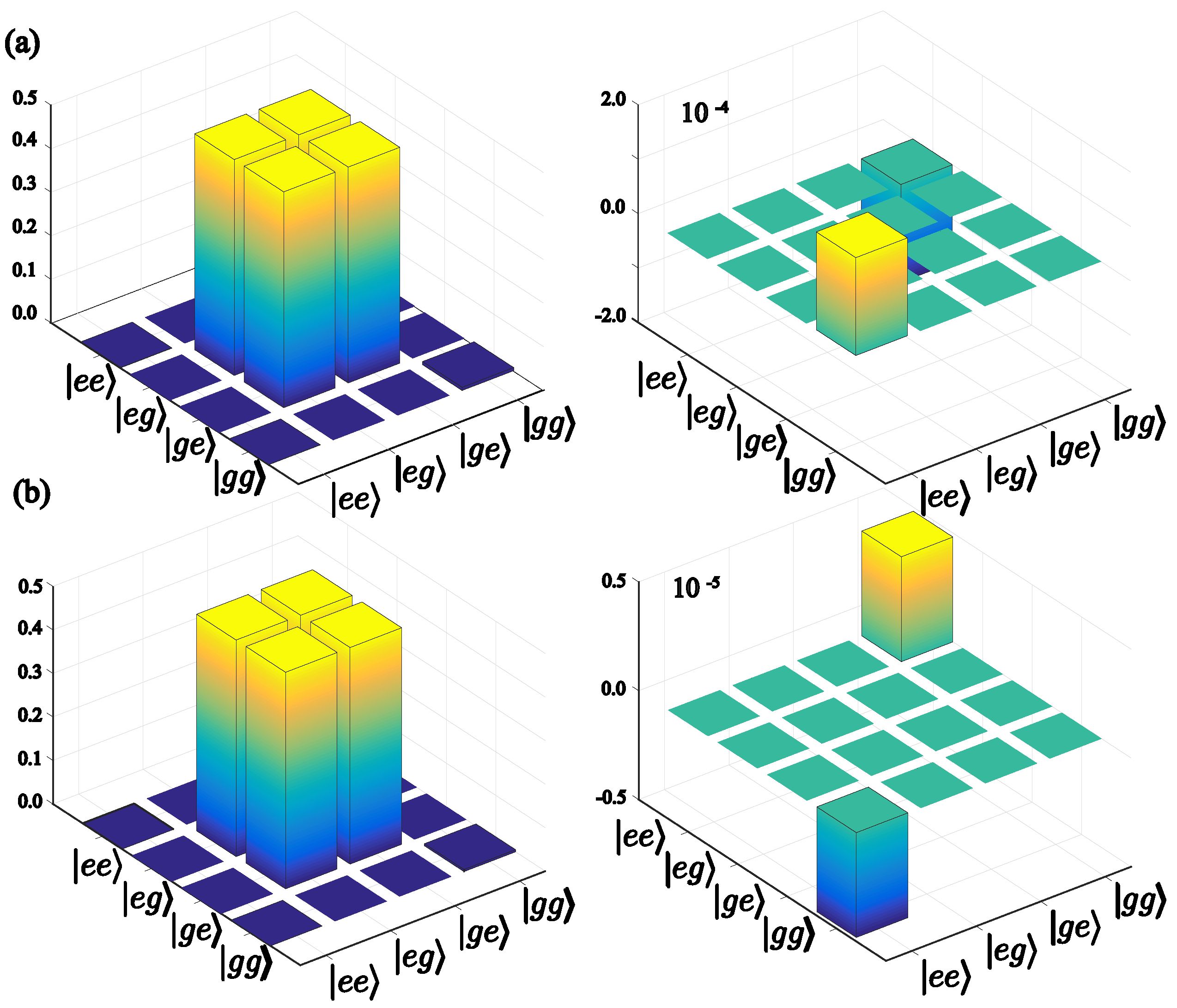
5. Copies of Density Matrices

In the above section, we have demonstrated that our system can generate identical copies of pure microwave photon states ($N=1,2,3$). Here, we demonstrate that even including loss mechanisms our protocol can still generate copies of density matrices with high fidelity. Since our proposal includes an ultrastrongly coupled light–matter system, the dissipative dynamics will be described by the master equation [73]

$$\begin{array}{ccc}\hfill \dot{\rho }\left(t\right)& =& i[\rho \left(t\right),\mathcal{H}]+\sum _{\ell =1}^N{\kappa }_{\ell }\mathcal{D}\left[b_{\ell }\right]\rho \left(t\right)+\sum _{\ell =1}^N{\kappa }_{\ell }\mathcal{D}\left[c_{\ell }\right]\rho \left(t\right)\hfill \\ & +& \sum _{E,E>E^{\prime }}({\mathsf{\Gamma }}_{\kappa }^{E{E}^{\prime }}+{\mathsf{\Gamma }}_{\gamma }^{E{E}^{\prime }}+{\mathsf{\Gamma }}_{{\gamma }_{\varphi }}^{E{E}^{\prime }})\mathcal{D}[|E,p\rangle \langle E^{\prime },p^{\prime }|]\rho \left(t\right).\hfill \end{array}$$

(11)

Here, $\mathcal{H}$ is the Hamiltonian of Equation (2) and $\mathcal{D}\left[O\right]\rho =1/2(2O\rho O^{†}-\rho O^{†}O-O^{†}O\rho )$ is the Liouvillian operator. Furthermore, ${\kappa }_{\ell }^n$ stands for photon loss rate for each cavity mode. ${\mathsf{\Gamma }}_{\kappa }^{E{E}^{\prime }}$, ${\mathsf{\Gamma }}_{\gamma }^{E{E}^{\prime }}$ and ${\mathsf{\Gamma }}_{{\gamma }_{\varphi }}^{E{E}^{\prime }}$ are the dressed decay rates associated with the quantum Rabi system, and they are defined as ${\mathsf{\Gamma }}_{\kappa }^{E{E}^{\prime }}=\frac{\kappa }{{\omega }_{\mathrm{cav}}}{\nu }_{E{E}^{\prime }}{|{\mathrm{X}}_{E{E}^{\prime }}|}^2$, ${\mathsf{\Gamma }}_{\gamma }^{E{E}^{\prime }}=\frac{\gamma }{{\omega }_q}{\nu }_{E{E}^{\prime }}{|{\sigma }_{E{E}^{\prime }}^x|}^2$ and ${\mathsf{\Gamma }}_{{\gamma }_{\varphi }}^{E{E}^{\prime }}=\frac{{\gamma }_{\varphi }}{{\omega }_q}{\nu }_{E{E}^{\prime }}{|{\sigma }_{E{E}^{\prime }}^z|}^2$, where $\kappa$, $\gamma$ and ${\gamma }_{\varphi }$ are the bare photon leakage, relaxation, and depolarizing noise rates, respectively. In the derivation of the master equation, it has to be assumed that the spectral densities describing the system–environment interactions correspond to an ohmic bath [74,75]. In this case, the impedance $Z\left(\omega \right)$ of each circuit element can be modelled as a resistor [76].

To study the robustness of our protocol under loss mechanisms, first we will examine the generation of copies of density matrices for the cases of $N=1,2,3$ two-mode cavities. As mentioned in the previous section, the whole system is initialized in the state $|\mathsf{\Psi }\left(0\right)\rangle =|0,+\rangle {⨂}_{\ell ,{\ell }^{\prime }}^N|0_{\ell },0_{{\ell }^{\prime }}\rangle$. Then, we let the system to evolve under Equation (11) for three different times: $t_S=\pi /\left(2{\mathcal{J}}_2^1\right)$, $t_B=\pi /\left(4{\mathcal{J}}_2^1\right)$, and $t_W=\pi /\left(6{\mathcal{J}}_2^1\right)$, for $N=1$, $N=2$, and $N=3$ two-mode cavities, respectively. Once the corresponding density matrix $\rho \left(t\right)$ is obtained, we trace over the quantum Rabi system and modes ${\omega }_2$ (${\omega }_1$) to obtain the reduced density matrix ${\rho }_{{\omega }_1}$ (${\rho }_{{\omega }_2}$), which contains only degrees of freedom associated with the mode ${\omega }_1$ (${\omega }_2$) distributed on different two-mode cavities.

Table 1. Summarized fidelity values between the states ${\rho }_{{\omega }_{\ell }}$ obtained through of the master Equation (17) with the fictitious states ${\rho }_{\mathrm{probe}}$ and ${\rho }_{\mathrm{tensor}}$ for the case where the quantum Rabi system is coupled to $n=\{1,2,3\}$ two-mode cavity.

	$\mathit{N}=1$	$\mathit{N}=2$	$\mathit{N}=3$
$\mathcal{F}({\rho }_{{\omega }_1},{\rho }_{{\omega }_2})$	0.9898	0.9818	0.9832
${\mathcal{F}}_S$	0.9892	-	-
${\mathcal{F}}_B$	-	0.9945	-
${\mathcal{F}}_W$	-	-	0.9904

, first row, shows the fidelity between both reduced density matrices $\mathcal{F}({\rho }_{{\omega }_1},{\rho }_{{\omega }_2})=\mathrm{Tr}\left({\rho }_{{\omega }_1}{\rho }_{{\omega }_2}\right)$. These results allow us to conclude that both quantum states are identical up to $99\%$ fidelity for a single cavity, and up to $98\%$ fidelity for two and three cavities. Table 1 also shows the fidelities of generating the states of Equation (9), which is, ${\mathcal{F}}_S=\mathrm{Tr}\left(\rho \left(t_S\right){\rho }_S\right)$, ${\mathcal{F}}_B=\mathrm{Tr}\left(\rho \left(t_B\right){\rho }_S\right)$, and ${\mathcal{F}}_W=\mathrm{Tr}\left(\rho \left(t_W\right){\rho }_S\right)$, where $\rho \left(t\right)$ have been numerically calculated from Equation (11). The high fidelities of our protocol are mainly due to the fast state generation times as compared with the loss rates. Our numerical calculations have been carried out with realistic circuit QED parameters at temperature $\mathrm{T}=15\mathrm{mK}$ [77]. For the quantum Rabi system decay rates, we consider values $\kappa =2\pi \times 0.10\mathrm{MHz}$, $\gamma =2\pi \times 15\mathrm{MHz}$ and ${\gamma }_{\varphi }=2\pi \times 7.69\mathrm{MHz}$ and for the cavities ${\kappa }_{\ell }^n=\kappa$.

The way to cease the system dynamics once we have obtained the entangled states is to tune the frequency of the two-level system forming the QRS. In such a case, the QRS becomes far off-resonant with the two-mode cavities, and the state does not evolve anymore. The time at which the system maintains the quantum state must be of the order of the decay time of the cavity. We do not expect that the decay time of the QRS affects this process, due to the fact that the QRS is in its ground state $|0,+\rangle$.

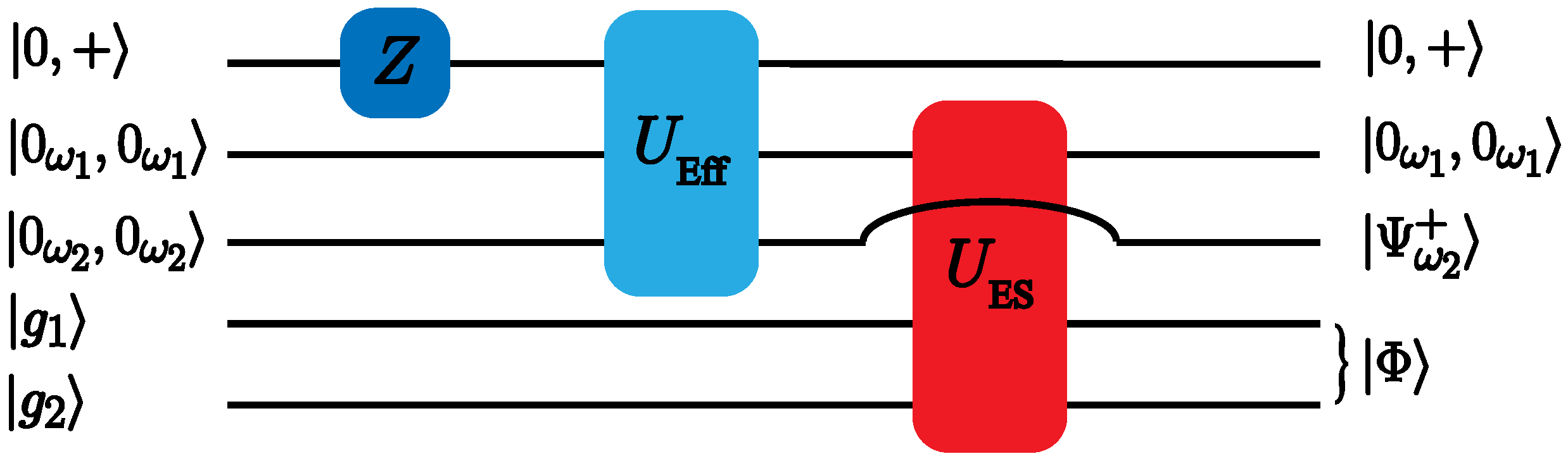
6. Entanglement Swapping between Distant Superconducting Qubits

In this section, we study the transfer of entanglement generated into the field modes towards distant superconducting circuits. Let us consider a pair of two-level systems coupled at the end of each cavity. As we shall see later in Section 7, our physical implementation will consider $\lambda /4$ transmission line resonators, and superconducting flux qubits to guarantee strong coupling between them. In such a case, we describe the system with the following Hamiltonian

$$\begin{array}{c}\hfill {\mathcal{H}}_{\mathrm{ES}}=\mathcal{H}+\sum _{\ell =1}^2\frac{{\omega }_{q\ell }^n}{2}{\sigma }_{\ell }^z+\sum _{\ell =1}^2{\lambda }_{\ell }{\sigma }_{\ell }^x(b_{\ell }+b_{\ell }^{†})+{\lambda }_{\ell }^{{}^{\prime }}{\sigma }_{\ell }^x(c_{\ell }+c_{\ell }^{†}),\end{array}$$

(12)

where $\mathcal{H}$ is the Hamiltonian defined in Equation (2). Moreover, ${\sigma }_{\ell }^x$ and ${\sigma }_{\ell }^z$ are Pauli matrices describing the two-level systems, $\{b_{\ell },c_{\ell }\},$ are the annihilation boson operators of the extended cavities. Additionally, ${\lambda }_{\ell }$, and ${\lambda }_{\ell }^{{}^{\prime }}$ are the coupling strength between the two-level system with the first and second field mode cavity, respectively. Depending on whether the two-level systems are resonant with either mode ${\omega }_{\ell }^1$ or ${\omega }_{\ell }^2$, the process with the coupling strength ${\lambda }_{\ell }$ or ${\lambda }_{\ell }^{{}^{\prime }}$ becomes dispersive $|{\omega }_{\ell }^1-{\omega }_{q\ell }^n|\gg \{{\lambda }_{\ell },{\lambda }_{\ell }^{{}^{\prime }}\}$ [78], and therefore we neglect it via the rotating wave approximation. The following master equation describes the system dynamics

$$\begin{array}{c}\hfill \dot{\rho }\left(t\right)=i[\rho \left(t\right),{\mathcal{H}}_{\mathrm{ES}}]+\sum _{\ell =1}^N{\gamma }_{\ell }\mathcal{D}\left[{\sigma }_{\ell }^{-}\right]\rho \left(t\right)+\sum _{\ell =1}^N{\gamma }_{{\varphi }_{\ell }}\mathcal{D}\left[{\sigma }_{\ell }^z\right]\rho \left(t\right).\end{array}$$

(13)

The last two terms describe the loss mechanisms acting on the two-level system, i.e., relaxation on the qubit at a rate $\gamma$ and depolarizing noise at rate ${\gamma }_{\varphi }$. The entanglement swapping protocol is the following; we initialize the whole system in its ground state

$$\begin{array}{c}\hfill {\rho }_0=|0,+\rangle \langle 0,+|\underset{\ell ,{\ell }^{\prime }}{\overset{N}{⨂}}|0_{\ell },0_{{\ell }^{\prime }}\rangle \langle 0_{\ell },0_{{\ell }^{\prime }}|\underset{\ell }{\overset{N}{⨂}}|g_{\ell }\rangle \langle g_{\ell }|.\end{array}$$

(14)

We dispersively couple the two-level systems with the field modes on the cavities ($|{\omega }_{\ell }^{1,2}-{\omega }_{q\ell }|\gg ({\lambda }_{\ell },{\lambda }_{\ell }^{{}^{\prime }})$) [78]. Then, we drive the quantum Rabi system to prepare it in the second excited state $|2,+\rangle$

$$\begin{array}{c}\hfill {\rho }_1=|2,+\rangle \langle 2,+|\underset{\ell ,{\ell }^{\prime }}{\overset{N}{⨂}}|0_{\ell },0_{{\ell }^{\prime }}\rangle \langle 0_{\ell },0_{{\ell }^{\prime }}|\underset{\ell }{\overset{N}{⨂}}|g_{\ell }\rangle \langle g_{\ell }|.\end{array}$$

(15)

This state is the initial condition of our scheme. Afterwards, we let the system evolve under the Hamiltonian in Equation (13). Due to the dispersive qubit–resonator interaction, the two-level systems do not evolve. After a time $t=\pi /\left(2{\mathcal{J}}_{\mathrm{eff}}\right)$, the density matrix of the system reads

$$\begin{array}{c}\hfill {\rho }_2=|0,+\rangle \langle 0,+|\underset{\ell }{\overset{N}{⨂}}|{\mathsf{\Psi }}_{{\omega }_{\ell }}^{+}\rangle \langle {\mathsf{\Psi }}_{{\omega }_{\ell }}^{+}|\underset{\ell }{\overset{N}{⨂}}|g_{\ell }\rangle \langle g_{\ell }|.\end{array}$$

(16)

The next step is to avoid the generated photons coming back to the quantum Rabi system. To achieve it, we tune far-off resonance the quantum Rabi system and the resonators by changing the qubit frequency that belongs to the quantum Rabi system. Afterwards, we put into resonance the external two-level system with either ${\omega }_{\ell }^1$ or ${\omega }_{\ell }^2$ field modes. In such a case, for a time $t=\pi /\left(2{\lambda }_{\ell }\right)$ ($t=\pi /\left(2{\lambda }_{\ell }^{{}^{\prime }}\right)$), the system evolves to

$$\begin{array}{ccc}\hfill {\rho }_3& =& |0,+\rangle \langle 0,+|\underset{\ell =1}{\overset{N}{⨂}}|0_{{\omega }_1^{\ell }}\rangle \langle 0_{{\omega }_1^{\ell }}|\otimes |{\mathsf{\Psi }}_{{\omega }_2^{\ell }}\rangle \langle {\mathsf{\Psi }}_{{\omega }_2^{\ell }}|\otimes |\mathsf{\Phi }\rangle \langle \mathsf{\Phi }|,\hfill \end{array}$$

(17)

$$\begin{array}{ccc}\hfill {\rho }_3& =& |0,+\rangle \langle 0,+|\underset{\ell =1}{\overset{N}{⨂}}|{\mathsf{\Psi }}_{{\omega }_2^{\ell }}\rangle \langle {\mathsf{\Psi }}_{{\omega }_2^{\ell }}|\otimes |0_{{\omega }_2^{\ell }}\rangle \langle 0_{{\omega }_2^{\ell }}|\otimes |\mathsf{\Phi }\rangle \langle \mathsf{\Phi }|.\hfill \end{array}$$

(18)

Here, $|\mathsf{\Phi }\rangle =(|g_1{e}_2\rangle +|e_1{g}_2\rangle )/\sqrt{2}$ is a Bell state of the pair of qubits. This protocol is illustrated in Figure 3. On the other hand, Figure 4 shows the real and imaginary part of the reduced density matrix for the pair of qubits after performing the protocol. As the figure shows, even though the loss mechanisms act on the system, the entanglement of the modes can be transferred to the qubits with high fidelity. For the two-level systems coupled to the first mode (${\omega }_1^{\ell }$), the fidelity is $\mathcal{F}=0.9960$, and $\mathcal{F}=0.9976$ when the qubit is resonant with the second mode (${\omega }_2^{\ell }$). This transfer occurs at the time scale of $t_{S_1}=23.08$ [ns] and $t_{S_2}=16.32$ [ns], respectively.

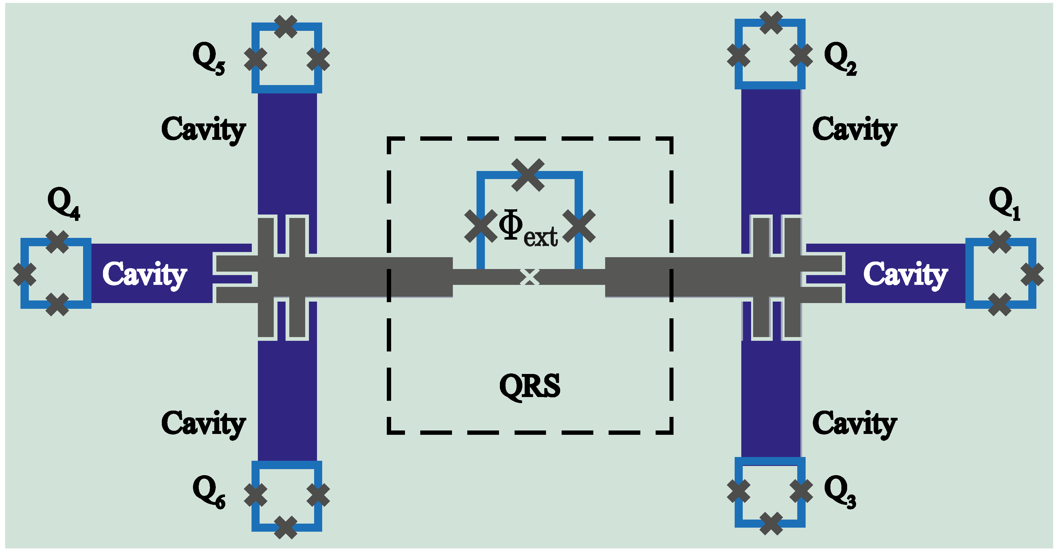
7. Implementation in Circuit QED

We depict the schematic implementation of our system in Figure 5. The circuit is composed of a non-uniform $\lambda /2$ transmission line resonator of length d galvanically coupled to a four-junction flux qubit at the middle of the resonator. The non-uniform shape of the resonator produces an increasing on its inductance in the vicinity of the qubit. In addition, the additional junction on the flux-qubit in the shared wire also produces an increase on the inductance of the resonator. As a result, the qubit-resonator coupling strength can achieve the USC regime [38]. Moreover, at the edges of this $\lambda /2$ resonator, one may couple up to six additional $\lambda /4$ transmission line resonator also of length d via capacitances. The capacitive coupling follows the same procedure as in Ref. [79]. In such a case, the finger pattern between the superconducting metal and the substrate form the capacitive coupling at the end of these resonators. The orthogonal arrangement between the two-mode cavity reduces the crosstalk between these resonators, reducing the cavity–cavity interaction. The Lagrangian representing this situation for $N=2$ resonators (extension to more two-mode resonators is straightforward) reads

$$\begin{array}{c}\hfill \mathcal{L}={\mathcal{L}}_{\mathrm{QRS}}+{\mathcal{L}}_{\mathrm{c}}+{\mathcal{L}}_I,\end{array}$$

(19)

where ${\mathcal{L}}_{\mathrm{QRS}}$ is the quantum Rabi system Lagrangian constituted by the $\lambda /2$ transmission line resonator coupled to a four-junction flux qubit, ${\mathcal{L}}_{\mathrm{c}}$ is the two-mode $\lambda /4$ transmission line resonator Lagrangian, whereas ${\mathcal{L}}_I$ stands for the resonator-resonator coupling Lagrangian obtained from the capacitive coupling. The quantum Rabi system Lagrangian is given by

$$\begin{array}{c}\hfill {\mathcal{L}}_{\mathrm{QRS}}={\int }_0^{d}dz\left[\frac{c}{2}{\left[{\partial }_t\psi (z,t)\right]}^2-\frac{1}{2l}{\left[{\partial }_z\psi (z,t)\right]}^2\right]+\sum _{k=1}^4\left[\frac{C_{J,k}}{2}{\dot{\phi }}_k^2+E_{J,k}cos\left(\frac{{\phi }_k}{{\varphi }_0}\right)\right].\end{array}$$

(20)

Here, $\psi (z,t)$, and ${\phi }_k$ correspond to the flux nodes for the $\lambda /2$ transmission line resonator and the four-Josephson flux qubit, respectively. These variables are related with the voltage drop through the specific branch component by means the relation $\psi (z,t)={\int }_{-\infty }^{t}V\left(t^{\prime }\right)d{t}^{\prime }$ [80,81]. Furthermore, c and l are the capacitance and inductance per unit length of the resonator, while $C_{J,k}$ and $E_{J,k}$ are the capacitance and energy describing the k-th Josephson junction. The two-mode resonator Lagrangian is given by

$$\begin{array}{c}\hfill {\mathcal{L}}_{\mathrm{c}}=\sum _{\ell =1}^{N=2}\left\{{\int }_0^{d}dz\left[\frac{c_{\ell }}{2}{\left[{\partial }_t{\varphi }_{\ell }(z,t)\right]}^2-\frac{1}{2l_{\ell }}{\left[{\partial }_z{\varphi }_{\ell }(z,t)\right]}^2\right]\right\}+\frac{C_r}{2}{\left[{\partial }_t{\varphi }_1(d,t)\right]}^2+\frac{C_r}{2}{\left[{\partial }_t{\varphi }_2(0,t)\right]}^2,\end{array}$$

(21)

where ${\varphi }_{\ell }$, $\ell =1,2$ is the flux node describing the ℓth two-mode resonator. Moreover, $c_{\ell }$, and $l_{\ell }$ stand for the capacitance and inductance per unit length of the ℓth two-mode resonator. Furthermore, $C_r$ is the coupling capacitance between the two-mode resonators with the QRS resonator. Finally, ${\mathcal{L}}_I$ is the interaction Lagrangian given by

$$\begin{array}{c}\hfill {\mathcal{L}}_I=-C_r\left[{\dot{\varphi }}_1(d,t)\dot{\psi }(0,t)+\dot{\psi }(d,t){\dot{\varphi }}_2(0,t)\right].\end{array}$$

(22)

As the two-level system with the resonator forming the quantum Rabi system is ultrastrongly coupled, we will expect in principle that the qubit also couples with the two-mode resonators. However, this does not occur due to the nature of the coupling between the flux-qubit with the transmission line resonator; as the $\lambda /2$ couples to the flux-qubit through the current, the latter should be placed at the position where the current reaches its maximum to achieve the USC coupling regime. In the $\lambda /2$ resonator, this position corresponds to the centre of the line. Thus, the edges of the QRS resonator have zero current and the qubit two-mode resonator coupling vanishes. As a result, the two-mode resonators couple to the QRS only through the resonator.

7.1. Rabi System Hamiltonian

For this derivation, we assume $E_{J,1}=E_{J,2}=E_J$, $E_{J,3}=\alpha E_J$ and $E_{J,4}=\gamma E_J$. Moreover, the fluxoid quantization relation on the superconducting loop is given by

$$\begin{array}{c}\hfill {\phi }_1-{\phi }_2+{\phi }_3+{\phi }_4=-2\pi f_x,\end{array}$$

(23)

where $f_x$ is the frustration parameter defined as $f_x={\varphi }_{\mathrm{ext}}/{\mathsf{\Phi }}_0$. On the other hand, we assume that the Josephson inductance of the fourth junction is smaller than the inductance of the flux-qubit loop, thus most of the current flowing through the resonator [38]. As a consequence, the qubit acts as a small perturbation of the transmission line resonator. Thus, the phase difference is given by ${\phi }_4=\Delta \psi$, where $\Delta \psi =\psi (z_i,t)-\psi (z_{i-1},t)$ corresponds to the phase difference of the $\lambda /2$ transmission line resonator at the position where the four Josephson junction is placed. Thus, the Lagrangian takes the following form

$$\begin{array}{ccc}\hfill {\mathcal{L}}_{\mathrm{QRS}}& =\hfill & {\int }_0^{d}dz\left[\frac{c}{2}{\left[{\partial }_t\psi (z,t)\right]}^2-\frac{1}{2l}{\left[{\partial }_z\psi (z,t)\right]}^2\right]+\frac{C_J}{2}\left[{\dot{{\phi }_1}}^2+{\dot{\phi }}_2^2+\alpha {(\dot{{\phi }_2}-\dot{{\phi }_1}-\Delta \dot{\psi })}^2+\gamma \Delta {\dot{\psi }}^2\right]\hfill \\ & +\hfill & E_J\left[cos\left(\frac{{\phi }_1}{{\varphi }_0}\right)+cos\left(\frac{{\phi }_2}{{\varphi }_0}\right)+\gamma cos\left(\frac{\Delta \psi }{{\varphi }_0}\right)+\alpha cos\left(\frac{{\phi }_2-{\phi }_1+{\varphi }_{\mathrm{ext}}-\Delta \psi }{{\varphi }_0}\right)\right].\hfill \end{array}$$

(24)

We are assuming the superconducting phase on the loop is well localized, thus the potential energy can be expanded in powers of $\Delta \psi /{\varphi }_0$ [51], allowing us to express the quantum Rabi system Lagrangian in the following form

$${\mathcal{L}}_{\mathrm{QRS}}={\mathcal{L}}_{\mathrm{r}}+{\mathcal{L}}_{\mathrm{q}}+{\mathcal{L}}_{\mathrm{qr}},$$

(25)

where ${\mathcal{L}}_{\mathrm{r}}$ is the Lagrangian of the resonator with an embedded junction

$$\begin{array}{c}\hfill {\mathcal{L}}_{\mathrm{r}}={\int }_0^{d}dz\left[\frac{c}{2}{\left[{\partial }_t\psi (z,t)\right]}^2-\frac{1}{2l}{\left[{\partial }_z\psi (z,t)\right]}^2\right]+\frac{C_J(\alpha +\gamma )}{2}\Delta \dot{\psi }+\gamma E_{J}cos\left(\frac{\Delta \psi }{{\varphi }_0}\right).\end{array}$$

(26)

Moreover, ${\mathcal{L}}_{\mathrm{q}}$ is the usual three-junction flux qubit Lagrangian [8]

$$\begin{array}{c}\hfill {\mathcal{L}}_{\mathrm{q}}=\frac{C_J}{2}\left[(1+\alpha )({\dot{{\phi }_1}}^2+{\dot{\phi }}_2^2)-2\alpha \dot{{\phi }_2}\dot{{\phi }_1}\right]+E_J\left[cos\left(\frac{{\phi }_1}{{\varphi }_0}\right)+cos\left(\frac{{\phi }_2}{{\varphi }_0}\right)+\alpha cos\left(\frac{{\phi }_2-{\phi }_1+{\varphi }_{\mathrm{ext}}}{{\varphi }_0}\right)\right].\end{array}$$

(27)

Finally, ${\mathcal{L}}_{\mathrm{qr}}$ is the qubit-resonator Lagrangian; this term has two contributions: capacitive and galvanic coupling, and reads

$$\begin{array}{c}\hfill {\mathcal{L}}_{\mathrm{qr}}=-\alpha C_J(\dot{{\phi }_1}+\dot{{\phi }_2})\Delta \dot{\psi }-\frac{\alpha E_J}{{\varphi }_0}sin\left(\frac{{\phi }_1-{\phi }_2+{\varphi }_{\mathrm{ext}}}{{\varphi }_0}\right)\Delta \psi .\end{array}$$

(28)

In the flux qubit, the capacitive energy is smaller than the inductive energy [38]. Thus, we neglect the capacitive term, obtaining

$$\begin{array}{c}\hfill {\mathcal{L}}_{\mathrm{qr}}=-\frac{\alpha E_J}{{\varphi }_0}sin\left(\frac{{\phi }_1-{\phi }_2+{\varphi }_x}{{\varphi }_0}\right)\Delta \psi .\end{array}$$

(29)

We obtain the Lagrangian for the transmission line resonator by computing its equation of motion. In such a case, the flux $\psi (z,t)$ obeys the wave equation whose solution for the $\lambda /2$ transmission line resonator is given by

$$\psi (z,t)=\sum _m{\mathcal{U}}_m\left(z\right){\mathcal{G}}_m\left(t\right),$$

(30)

$$\psi (z,t)=\sum _m\left[A_{m}cos{k}_m(z-d/2)+B_{m}sin{k}_m(z+d/2)\right]{\mathcal{G}}_m\left(t\right),$$

(31)

where $k_m$ is the wave vector of the resonator with the embedded junction, which is obtained through the dispersion relation

$$\begin{array}{c}\hfill k_{m}tan\left(\frac{k_{m}d}{2}\right)=\frac{2l}{L_J}\left[1-{\left(\frac{v{k}_m}{{\omega }_p}\right)}^2\right],\end{array}$$

(32)

with $v=\sqrt{1/lc}$ is the transmission line resonator wave velocity, $L_J=\gamma {\varphi }_0^2/E_J$ is the Josephson inductance. In addition, ${\omega }_p=1/\sqrt{L_J{C}_J}$ is the plasma frequency of the embedded junction. Replacing the flux $\psi (z,t)$ on the Lagrangian given in Equation (21), we arrive at

$$\begin{array}{c}\hfill {\mathcal{L}}_{\mathrm{r}}=\sum _m\left[\frac{{\eta }_m\dot{{\mathcal{G}}_m}{\left(t\right)}^2}{2}-\frac{{\eta }_m^2{\omega }_m^2{\mathcal{G}}_m^2\left(t\right)}{2}\right],\end{array}$$

(33)

where ${\eta }_m$ is the effective capacitance [17]. By applying the Legendre transformation, we arrive at the classical Hamiltonian

$$\begin{array}{c}\hfill {\mathcal{H}}_{\mathrm{r}}=\sum _m\left[\frac{{\mathsf{\Pi }}_m^2}{2{\eta }_m}+\frac{{\eta }_m^2{\omega }_m^2{G}_m^2}{2}\right].\end{array}$$

(34)

Here, ${\mathsf{\Pi }}_m=\partial \mathcal{L}/\partial \left[{\dot{G}}_m\right]$ is the canonical conjugate momenta. We proceed to quantize the Hamiltonian promoting the following operators:

$$\begin{array}{c}\hfill {\mathsf{\Pi }}_m=\sqrt{\frac{\hslash }{2{\eta }_m{\omega }_m}}(a_m^{†}+a_m),\end{array}$$

(35)

$$\begin{array}{c}\hfill G_m=i\sqrt{\frac{\hslash {\eta }_m{\omega }_m}{2}}(a_m^{†}-a_m).\end{array}$$

(36)

Replacing these operators in the Hamiltonian ${\mathcal{H}}_r$ we arrive at the transmission line resonator quantum Hamiltonian

$$\begin{array}{c}\hfill {\mathcal{H}}_{\mathrm{r}}=\sum _m\hslash {\omega }_m\left(a_m^{†}{a}_m+\frac{1}{2}\right).\end{array}$$

(37)

Now, let us consider the Lagrangian of the four-junction flux qubit given in Equation (27). Close to the degeneracy point ${\varphi }_x={\varphi }_0/2$, the system can be truncated to the two lowest eigenstates, whose Hamiltonian is given by

$$\begin{array}{c}\hfill {\mathcal{H}}_{\mathrm{q}}=\frac{\hslash {\omega }_{\mathrm{q}}}{2}{\sigma }^z,\end{array}$$

(38)

where ${\omega }_{\mathrm{q}}=\sqrt{{\Delta }^2+{\epsilon }^2}$, with $\Delta$ the qubit gap, and $\epsilon =2I_p({\varphi }_x-{\varphi }_0/2)$, where $I_p$ is the persistent current on the superconducting loop. Furthermore, the interacting Lagrangian given in Equation (29) can be written in the two-level basis, in such case, the quantized Hamiltonian reads

$$\begin{array}{ccc}\hfill {\mathcal{H}}_{\mathrm{qr}}& =& i\frac{\alpha E_J\Delta {\mathcal{U}}_m}{{\varphi }_0}\sqrt{\frac{\hslash {\eta }_m{\omega }_m}{2}}{S}_{01}{\sigma }^x(a_m-a_m^{†}),\hfill \end{array}$$

(39)

$$\begin{array}{ccc}\hfill S_{01}& =& \langle 0|\left[sin\left(\frac{{\phi }_1-{\phi }_2+{\varphi }_x}{{\varphi }_0}\right)\right]|1\rangle .\hfill \end{array}$$

(40)

Thus, the quantum Rabi Hamiltonian is given by

$$\begin{array}{c}\hfill {\mathcal{H}}_{\mathrm{QRS}}=\sum _m\hslash {\omega }_m{a}_m^{†}{a}_m+\frac{\hslash {\omega }_q}{2}{\sigma }^z+\hslash \sum _m{g}_m{\sigma }^x(a_m^{†}+a_m).\end{array}$$

(41)

Notice that the coupling strength between the transmission line resonator and the artificial atom depends on two factors: the position at which the two-level system is placed, and the nature of the coupling, i.e., galvanic or capacitive. In our case, as the artificial atom corresponds to a flux-qubit, it is coupled to the current on the transmission line resonator. As a consequence, the two-level system only couples to even modes because the odd modes have a node [39] in the flux qubit position as illustrated in Figure 6a. The spectrum of the multi-mode Rabi system is depicted in Figure 6b. Notice that the energy spectrum of the multimode quantum Rabi system preserves the parity symmetry exhibited by the single mode quantum Rabi system (see Figure 1). Furthermore, for a wide range of coupling strength g, the low-lying energy states exhibit the same selection rules observed in the single mode Rabi system. Thus, by adding more complexity to the mediator system (quantum Rabi system), our proposed generation scheme is still useful due to the preserve of the selection rules on the system:

$$\begin{array}{c}\hfill {\mathcal{H}}_{\mathrm{QRS}}=\hslash {\omega }_{\mathrm{cav}}{a}^{†}a+\frac{\hslash {\omega }_q}{2}{\sigma }^z+\hslash g{\sigma }^x(a^{†}+a).\end{array}$$

(42)

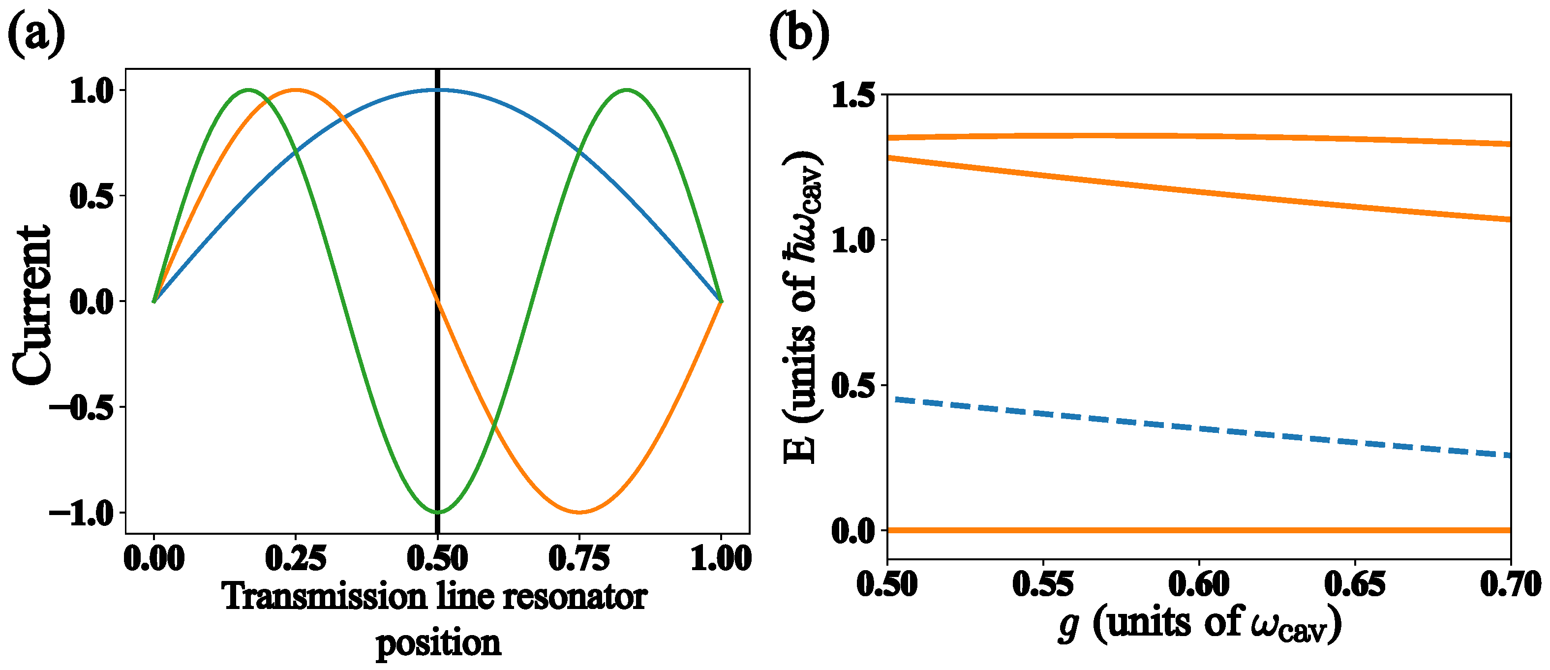
7.2. Multimode Cavity Hamiltonian

To obtain the Hamiltonian of the two-mode cavities, let us consider the Lagrangian given in Equation (21) for $N=2$ resonators

$$\begin{array}{c}\hfill {\mathcal{L}}_{\mathrm{c}}=\sum _{\ell =1}^{N=2}\left\{{\int }_0^{d}dz\left[\frac{c_{\ell }}{2}{\left[{\partial }_t{\varphi }_{\ell }(z,t)\right]}^2-\frac{1}{2l_{\ell }}{\left[{\partial }_z{\varphi }_{\ell }(z,t)\right]}^2\right]\right\}+\frac{C_r}{2}{\left[{\partial }_t{\varphi }_1(d,t)\right]}^2+\frac{C_r}{2}{\left[{\partial }_t{\varphi }_2(0,t)\right]}^2.\end{array}$$

(43)

For the specific implementation, we consider boundary conditions defining a $\lambda /4$ resonator, where the current at the ends where the two-mode resonator coupled to the QRS resonator is zero, and the voltage reaches its maximum. These conditions are given by

$$\begin{array}{c}\hfill -{\partial }_z{\varphi }_1(0,t)=-{\partial }_z{\varphi }_2(d,t)=0,\end{array}$$

(44)

$$\begin{array}{c}\hfill {\partial }_t{\varphi }_1(d,t)={\partial }_t{\varphi }_2(0,t)=0.\end{array}$$

(45)

By solving the wave equation with the previous boundary conditions, we obtain the expression for the flux on the ℓth $\lambda /4$ transmission line resonator

$$\begin{array}{c}\hfill {\varphi }_1=\sum _n{A}_{n}cos\left(q_{n,\ell }z\right)G_n\left(t\right);{\varphi }_2=\sum _n{B}_{n}cos{q}_{n,\ell }(z-d)G_n\left(t\right),\end{array}$$

(46)

where $G_n$ satisfy the time-dependent part of the wave equation. Moreover, $q_{n,\ell }$ corresponds to a quasi-momentum satisfying the following dispersion relation:

$$\begin{array}{c}\hfill q_{n,\ell }=\frac{1}{v_{\ell }{l}_{\ell }{C}_r}cot\left(q_{n}d\right).\end{array}$$

(47)

By replacing the expression of the fluxes ${\varphi }_1$, and ${\varphi }_2$ and performing the Legendre transformation, we arrive at the quantum $\lambda /4$ transmission line resonator Hamiltonian

$$\begin{array}{c}\hfill {\mathcal{H}}_{\mathrm{c}}=\sum _{\ell =1}^N\sum _n\hslash {\omega }^{\ell ,n}\left(b_{\ell ,n}^{†}{b}_{\ell ,n}+\frac{1}{2}\right).\end{array}$$

(48)

Here, the index n runs over all the mode on the transmission line, whereas the index ℓ stands for the number of multi-mode resonator coupled to the QRS. Notice that in principle all the modes of the $\lambda /4$ are involved in the system dynamics. However, numerical simulations show that, due to the resonance condition on our system, the field mode greater than three does not induce dynamics in the system. Thus, by keeping the notation given in Equation (1), we rewrite the Hamiltonian in Equation (48) as follows:

$$\begin{array}{c}\hfill {\mathcal{H}}_{\mathrm{c}}=\sum _{\ell =1}^N\left[\hslash {\omega }_1^{\ell }\left(b_{\ell }^{†}{b}_{\ell }+\frac{1}{2}\right)+\hslash {\omega }_2^{\ell }\left(c_{\ell }^{†}{c}_{\ell }+\frac{1}{2}\right)\right],\end{array}$$

(49)

where ${\omega }_1^{\ell }$ and ${\omega }_2^{\ell }$ correspond to the frequency of the first and second field mode of the ℓth $\lambda /4$, respectively. Likewise, $b_{\ell }$ and $c_{\ell }$ are the boson operator for the first and second field mode, respectively.

7.3. Complete Model

With the Hamiltonian of the free system already obtained in the previous section, we are able to write the interacting Hamiltonian of the complete system. Before the application of the Legendre transformation, the Lagrangian in Equation (22) turns on the interaction Hamiltonian

$$\begin{array}{c}\hfill {\mathcal{H}}_I=C_r\left[{\dot{\varphi }}_1(d,t)\dot{\psi }(0,t)+\dot{\psi }(d,t){\dot{\varphi }}_2(0,t)\right].\end{array}$$

(50)

By replacing the expression of the fluxes $\psi (z,t)$ and ${\varphi }_{\ell }(z,t)$ already obtained, we arrive at the quantum interaction Hamiltonian

$$\begin{array}{ccc}\hfill {\mathcal{H}}_I& =& \sum _{\ell =1}^N\sum _m\left[J_1^{\ell ,m}(b_{\ell }^{†}+b_{\ell })+J_2^{\ell ,m}(c_{\ell }^{†}+c_{\ell })\right](a_m+a_m^{†}),\hfill \end{array}$$

(51)

$$\begin{array}{ccc}\hfill J_1^{\ell ,m}& =& \frac{\hslash C_r}{2}\sqrt{\frac{1}{{\eta }_m{\overline{\eta }}_{n,\ell }{\omega }_m{\omega }_1^{\ell }}}\psi \left(0\right){\varphi }_1\left(d\right),\hfill \end{array}$$

(52)

$$\begin{array}{ccc}\hfill J_2^{\ell ,m}& =& \frac{\hslash C_r}{2}\sqrt{\frac{1}{{\eta }_m{\overline{\eta }}_{n,\ell }{\omega }_m{\omega }_2^{\ell }}}\psi \left(d\right){\varphi }_1\left(0\right).\hfill \end{array}$$

(53)

Here, ${\overline{\eta }}_{n,\ell }$ is the effective capacitance of the $\lambda /4$ transmission line resonator. Notice that capacitive coupling strength between resonators is commonly at least one order of magnitude smaller than the bare frequency of the field mode frequency. Thus, for resonator in the Giga Hertz regime, coupling strength $J_{1,2}^{\ell ,m}$ are within the Mega Hertz regime. In the single mode approximation for the QRS resonator, we obtain

$$\begin{array}{c}\hfill {\mathcal{H}}_I=\sum _{\ell =1}^N\left[J_1^{\ell }(b_{\ell }^{†}+b_{\ell })+J_2^{\ell }(c_{\ell }^{†}+c_{\ell })\right](a+a^{†}).\end{array}$$

(54)

Thus, the complete system Hamiltonian is given by

$$\begin{array}{ccc}\hfill \mathcal{H}& =& \hslash {\omega }_{\mathrm{cav}}{a}^{†}a+\frac{\hslash {\omega }_q}{2}{\sigma }^z+\hslash g{\sigma }^x(a^{†}+a)+\sum _{\ell =1}^N\left[\hslash {\omega }_1^{\ell }\left(b_{\ell }^{†}{b}_{\ell }+\frac{1}{2}\right)+\hslash {\omega }_2^{\ell }\left(c_{\ell }^{†}{c}_{\ell }+\frac{1}{2}\right)\right]\hfill \\ & +& \sum _{\ell =1}^N\left[J_1^{\ell }(b_{\ell }^{†}+b_{\ell })+J_2^{\ell }(c_{\ell }^{†}+c_{\ell })\right](a+a^{†}).\hfill \end{array}$$

(55)

To assure that our approximations are valid, we compute the system dynamics for the case of $N=1$ resonator that contains three modes. As we see in Figure 7, due to the third mode, it is not resonant with the QRS energy transition. This contribution does not affect the generation scheme.

7.4. Driving the Superconducting Qubit

We can drive the two-level system by applying a time-dependent magnetic field on the superconducting loop (see Figure 5). In such case, the energy gap ${\omega }_q$ can be expressed as

$$\begin{array}{c}\hfill {\omega }_q\left(t\right)=\sqrt{{\Delta }^2+{\epsilon }^2\left(t\right)},\end{array}$$

(56)

where $\epsilon \left(t\right)={\epsilon }_{\mathrm{DC}}+{\epsilon }_{\mathrm{AC}}cos\left({\omega }_{L}t\right)$ is the time-dependent energy on the system, which contains DC and AC contributions [82]. For ${\epsilon }_{DC}\gg {\epsilon }_{AC}$, we can write the flux-qubit energy as

$$\begin{array}{c}\hfill {\omega }_q=\sqrt{{\Delta }^2+{\epsilon }_{DC}^2}+\frac{{\epsilon }_{\mathrm{DC}}{\epsilon }_{\mathrm{AC}}}{\sqrt{{\Delta }^2+{\epsilon }_{DC}^2}}cos\left({\omega }_{L}t\right).\end{array}$$

(57)

Thus, the flux-qubit driving Hamiltonian is given by

$$\begin{array}{c}\hfill {\mathcal{H}}_q\left(t\right)=\frac{{\omega }_q}{2}{\sigma }^z+\mathsf{\Omega }cos\left({\omega }_{L}t\right){\sigma }^z.\end{array}$$

(58)

8. Conclusions

In summary, we have shown the usefulness of the quantum Rabi system to generate photons under suitable configuration. Based on the selection rules and the anharmonicity present in the quantum Rabi system, it is possible to find the specific matching condition for producing two-photon processes, analogous to the observed in the parametric frequency conversion. This condition allows us to generate in a deterministic manner uncorrelated or correlated photon states, Bell and W states. The protocol mentioned above, together with available optical to microwave photon converter technologies, may be a useful resource to perform tasks as distributed quantum computing or quantum cryptography.

On the other hand, the proposed protocol could work as a quantum random number generator (QRNG) in the microwave regime. Unlike the optical regime where QRNGs are based on single mode and polarization states of photons, our proposal considers two-mode states of photons. As a consequence, we observe a quadratic increase in the amount of possible quantum random numbers that would be generated in comparison with the single-mode case. Moreover, due to the fact that our system generates simultaneously identical maximally entangled photonic states of different frequency, this state resembles a $N^2$-side dice, where each side is associated with the probability to find the photons of frequency ${\omega }_1$ and ${\omega }_2$ in one of the two modes in N cavities. Thus, the multiphoton process mediated by the quantum Rabi system occurring on the two-mode cavities provides an efficient way to produce quantum random numbers. This efficiency relies on two main aspects of our protocol. The former is concerned with the collective effect producing a decrease of the generation time as the number of cavities increases, permitting the avoidance of the bias produced by the interaction of the system with the environment. The latter concerns the multimode configuration of our scheme. As we previously mentioned, the inclusion of the multimode systems allows us to increase the amount of possible quantum random numbers as the number of devices required decrease. Finally, we have also proposed a possible experimental implementation of our scheme considering near-term technology on circuit quantum electrodynamics in the ultrastrong coupling regime.

References

1. You, J.Q.; Nori, F. Atomic physics and quantum optics using superconducting circuits. Nature 2011, 474, 589–597. [Google Scholar] [CrossRef] [PubMed] [Green Version]
2. Houck, A.A.; Türeci, H.E.; Koch, J. On-chip quantum simulation with superconducting circuits. Nat. Phys. 2012, 8, 292–299. [Google Scholar] [CrossRef]
3. Devoret, M.H.; Schoelkopf, R.J. Superconducting circuits for quantum information: An outlook. Science 2013, 339, 1169–1174. [Google Scholar] [CrossRef]
4. Wallraff, A.; Schuster, D.I.; Blais, A.; Frunzio, L.; Huang, R.S.; Majer, J.; Kumar, S.; Girvin, S.M.; Schoelkopf, R.J. Strong coupling of a single photon to a superconducting qubit using circuit quantum electrodynamics. Nature 2004, 431, 162–167. [Google Scholar] [CrossRef] [PubMed] [Green Version]
5. Blais, A.; Huang, R.S.; Wallraff, A.; Girvin, S.M.; Schoelkopf, R.J. Cavity quantum electrodynamics for superconducting electrical circuits: An architecture for quantum computation. Phys. Rev. A 2004, 69, 062320. [Google Scholar] [CrossRef] [Green Version]
6. Nakamura, Y. Microwave quantum photonics in superconducting circuits. In Proceedings of the IEEE Photonics Conference 2012, Burlingame, CA, USA, 23–27 September 2012; pp. 544–545. [Google Scholar]
7. Gu, X.; Kockum, A.F.; Miranowicz, A.; Liu, Y.X.; Nori, F. Microwave photonics with superconducting quantum circuits. Phys. Rep. 2017, 718–719, 1–102. [Google Scholar] [CrossRef]
8. Orlando, T.P.; Mooij, J.E.; Tian, L.; van der Wal, C.H.; Levitov, L.S.; Lloyd, S.; Mazo, J.J. Superconducting persistent-current qubit. Phys. Rev. B 1999, 60, 15398–15413. [Google Scholar] [CrossRef] [Green Version]
9. Koch, J.; Terri, M.Y.; Gambetta, J.; Houck, A.A.; Schuster, D.I.; Majer, J.; Blais, A.; Devoret, M.H.; Girvin, S.M.; Schoelkopf, R.J. Charge-insensitive qubit design derived from the Cooper pair box. Phys. Rev. A 2007, 76, 042319. [Google Scholar] [CrossRef] [Green Version]
10. Göppl, M.; Fragner, A.; Baur, M.; Bianchetti, R.; Filipp, S.; Leek, J.M.F.P.J.; Puebla, G.; Steffen, L.; Wallraff, A. Coplanar waveguide resonators for circuit quantum electrodynamics. J. Appl. Phys. 2008, 104, 113904. [Google Scholar] [CrossRef] [Green Version]
11. Abdumalikov, A.A.; Astafiev, O.; Zagoskin, A.M.; Pashkin, Y.A.; Nakamura, Y.; Tsai, J.S. Electromagnetically induced transparency on a single artificial atom. Phys. Rev. Lett. 2010, 104, 193601. [Google Scholar] [CrossRef]
12. Lang, C.; Bozyigit, D.; Eichler, C.; Steffen, L.; Fink, J.M.; Abdumalikov, A.A., Jr.; Baur, M.; Filipp, S.; Da Silva, M.P.; Blais, A.; et al. Observation of resonant photon blockade at microwave frequencies using correlation function measurements. Phys. Rev. Lett. 2011, 106, 243601. [Google Scholar] [CrossRef]
13. Goetz, J.; Deppe, F.; Fedorov, K.G.; Eder, P.; Fischer, M.; Pogorzalek, S.; Xie, E.; Marx, A.; Gross, R. Parity-Engineered Light-Matter Interaction. Phys. Rev. Lett. 2018, 121, 060503. [Google Scholar] [CrossRef]
14. Bergeal, N.; Vijay, R.; Manucharyan, V.E.; Siddiqi, I.; Schoelkopf, R.J.; Girvin, S.M.; Devoret, M.H. Analog information processing at the quantum limit with a Josephson ring modulator. Nat. Phys. 2010, 6, 296–302. [Google Scholar] [CrossRef] [Green Version]
15. Boissonneault, M.; Gambetta, J.M.; Blais, A. Improved superconducting qubit readout by qubit-induced nonlinearities. Phys. Rev. Lett. 2010, 105, 100504. [Google Scholar] [CrossRef] [PubMed]
16. Bourassa, J.; Beaudoin, F.; Gambetta, J.M.; Blais, A. Josephson-junction-embedded transmission-line resonators: From Kerr medium to in-line transmon. Phys. Rev. A 2012, 86, 013814. [Google Scholar] [CrossRef]
17. Leib, M.; Deppe, F.; Marx, A.; Gross, R.; Hartmann, M.J. Networks of nonlinear superconducting transmission line resonators. New J. Phys. 2012, 14, 075024. [Google Scholar] [CrossRef] [Green Version]
18. Hoi, I.-C.; Kockum, A.F.; Palomaki, T.; Stace, T.M.; Fan, B.; Tornberg, L.; Sathyamoorthy, S.R.; Johansson, G.; Delsing, P.; Wilson, C.M. Giant Cross–Kerr Effect for Propagating Microwaves Induced by an Artificial Atom. Phys. Rev. Lett. 2013, 111, 053601. [Google Scholar] [CrossRef] [PubMed]
19. Marquardt, F. Efficient on-chip source of microwave photon pairs in superconducting circuit QED. Phys. Rev. B 2007, 76, 205416. [Google Scholar] [CrossRef]
20. Koshino, K. Down-conversion of a single photon with unit efficiency. Phys. Rev. A 2009, 79, 013804. [Google Scholar] [CrossRef]
21. Liu, Y.X.; Sun, H.C.; Peng, Z.H.; Miranowicz, A.; Tsai, J.S.; Nori, F. Controllable microwave three-wave mixing via a single three-level superconducting quantum circuit. Sci. Rep. 2014, 4, 7289. [Google Scholar] [CrossRef] [Green Version]
22. Sánchez-Burillo, E.; Martín-Moreno, L.; García-Ripoll, J.J.; Zueco, D. Full two-photon down-conversion of a single photon. Phys. Rev. A 2016, 94, 053814. [Google Scholar] [CrossRef]
23. Yurke, B.; Corruccini, L.R.; Kaminsky, P.G.; Rupp, L.W.; Smith, A.D.; Silver, A.H.; Simon, R.W.; Whittaker, E.A. Observation of parametric amplification and deamplification in a Josephson parametric amplifier. Phys. Rev. A 1989, 39, 2519–2533. [Google Scholar] [CrossRef]
24. Everitt, M.J.; Clark, T.D.; Stiffell, P.B.; Vourdas, A.; Ralph, J.F.; Prance, R.J.; Prance, H. Superconducting analogs of quantum optical phenomena: Macroscopic quantum superpositions and squeezing in a superconducting quantum-interference device ring. Phys. Rev. A 2004, 69, 043804. [Google Scholar] [CrossRef]
25. Zagoskin, A.M.; Il’chev, E.; McCutcheon, M.W.; Young, J.F.; Nori, F. Controlled generation of squeezed states of microwave radiation in a superconducting resonant circuit. Phys. Rev. Lett. 2008, 101, 253602. [Google Scholar] [CrossRef]
26. Moon, K.; Girvin, S.M. Theory of microwave parametric down-conversion and squeezing using circuit QED. Phys. Rev. Lett. 2005, 95, 140504. [Google Scholar] [CrossRef]
27. Didier, N.; Qassemi, F.; Blais, A. Perfect squeezing by damping modulation in circuit quantum electrodynamics. Phys. Rev. A 2014, 89, 013820. [Google Scholar] [CrossRef]
28. Strauch, F.W. All-resonant control of superconducting resonators. Phys. Rev. Lett. 2012, 109, 210501. [Google Scholar] [CrossRef] [PubMed]
29. Zhao, Y.-J.; Wang, C.; Zhu, X.; Liu, Y.-X. Engineering entangled microwave photon states through multiphoton interactions between two cavity fields and a superconducting qubit. Sci. Rep. 2016, 6, 23646. [Google Scholar] [CrossRef] [Green Version]
30. Merkel, S.T.; Wilhelm, F.K. Generation and detection of NOON states in superconducting circuits. New J. Phys. 2010, 12, 093036. [Google Scholar] [CrossRef] [Green Version]
31. Strauch, F.W.; Jacobs, K.; Simmonds, R.W. Arbitrary Control of Entanglement between two Superconducting Resonators. Phys. Rev. Lett. 2010, 105, 050501. [Google Scholar] [CrossRef] [PubMed]
32. Wang, H.; Mariantoni, M.; Bialczak, R.C.; Lenander, M.; Lucero, E.; Neeley, M.; O’Connell, A.D.; Sank, D.; Weides, M.; Wenner, J.; et al. Deterministic Entanglement of Photons in Two Superconducting Microwave Resonators. Phys. Rev. Lett. 2011, 106, 060401. [Google Scholar] [CrossRef] [Green Version]
33. Gasparinetti, S.; Pechal, M.; Besse, J.C.; Mondal, M.; Eichler, C.; Wallraff, A. Correlations and entanglement of microwave photons emitted in a cascade decay. Phys. Rev. Lett. 2017, 119, 140504. [Google Scholar] [CrossRef] [PubMed]
34. Campagne-Ibarcq, P.; Zalys-Geller, E.; Narla, A.; Shankar, S.; Reinhold, P.; Burkhart, L.D.; Axline, C.J.; Pfaff, W.; Frunzio, L.; Schoelkopf, R.J.; et al. Deterministic remote entanglement of superconducting circuits through microwave two-photon transitions. Phys. Rev. Lett. 2018, 120, 200501. [Google Scholar] [CrossRef] [PubMed]
35. Rosenblum, S.; Gao, Y.Y.; Reinhold, P.; Wang, C.; Axline, C.J.; Frunzio, L.; Girvin, S.M.; Jiang, L.; Mirrahimi, M.; Devoret, M.H.; et al. A CNOT gate between multiphoton qubits encoded in two cavities. Nat. Commun. 2018, 9, 652. [Google Scholar] [CrossRef] [PubMed]
36. Narla, A.; Shankar, S.; Hatridge, M.; Leghtas, Z.; Sliwa, K.M.; Zalys-Geller, E.; Mundhada, S.O.; Pfaff, W.; Frunzio, L.; Shoelkopf, R.J.; et al. Robust concurrent remote entanglement between two superconducting qubits. Phys. Rev. X 2016, 6, 031036. [Google Scholar] [CrossRef]
37. Kurpiers, P.; Magnard, P.; Walter, T.; Royer, B.; Pechal, M.; Heinsoo, J.; Salathé, Y.; Akin, A.; Storz, S.; Besse, J.C.; et al. Deterministic Quantum State Transfer and Generation of Remote Entanglement using Microwave Photons. Nature 2018, 558, 264–267. [Google Scholar] [CrossRef]
38. Bourassa, J.; Gambetta, J.M.; Abdumalikov, A.A.; Astafiev, O.; Nakamura, Y.; Blais, A. Ultrastrong coupling regime of cavity QED with phase-biased flux qubits. Phys. Rev. A 2009, 80, 032109. [Google Scholar] [CrossRef]
39. Niemczyk, T.; Deppe, F.; Huebl, H.; Menzel, E.P.; Hocke, F.; Schwarz, M.J.; García-Ripoll, J.J.; Zueco, D.; Hümmer, T.; Solano, E.; et al. Circuit quantum electrodynamics in the ultrastrong-coupling regime. Nat. Phys. 2010, 6, 772–776. [Google Scholar] [CrossRef] [Green Version]
40. Forn-Díaz, P.; Lisenfeld, J.; Marcos, D.; García-Ripoll, J.J.; Solano, E.; Harmans, C.J.P.M.; Mooij, J.E. Observation of the Bloch-Siegert shift in a qubit-oscillator system in the ultrastrong coupling regime. Phys. Rev. Lett. 2010, 105, 237001. [Google Scholar] [CrossRef]
41. Andersen, C.K.; Blais, A. Ultrastrong coupling dynamics with a transmon qubit. New J. Phys. 2017, 19, 023022. [Google Scholar] [CrossRef] [Green Version]
42. Forn-Díaz, P.; García-Ripoll, J.J.; Peropadre, B.; Orgiazzi, J.L.; Yurtalan, M.A.; Belyansky, R.; Wilson, C.M.; Lupascu, A. Ultrastrong coupling of a single artificial atom to an electromagnetic continuum in the nonperturbative regime. Nat. Phys. 2017, 13, 39–43. [Google Scholar] [CrossRef]
43. Martínez, J.P.; Léger, S.; Gheeraert, N.; Dassonneville, R.; Planat, L.; Foroughi, F.; Krupko, Y.; Buisson, O.; Naud, C.; Hasch-Guichard, W.; et al. A tunable Josephson platform to explore many-body quantum optics in circuit-QED. arXiv, 2018; arXiv:1802.00633. [Google Scholar]
44. Casanova, J.; Romero, G.; Lizuain, I.; García-Ripoll, J.J.; Solano, E. Deep Strong Coupling Regime of the Jaynes-Cummings Model. Phys. Rev. Lett. 2010, 105, 263603. [Google Scholar] [CrossRef]
45. Yoshihara, F.; Fuse, T.; Ashhab, S.; Kakuyanagi, K.; Saito, S.; Semba, K. Superconducting qubit-oscillator circuit beyond the ultrastrong-coupling regime. Nat. Phys. 2017, 13, 44–47. [Google Scholar] [CrossRef]
46. Forn-Díaz, P.; Lamata, L.; Rico, E.; Kono, J.; Solano, E. Ultrastrong coupling regimes of light–matter interaction. arXiv, 2018; arXiv:1804.09275. [Google Scholar]
47. Kockum, A.F.; Miranowicz, A.; de Liberato, S.; Savasta, S.; Nori, F. Ultrastrong coupling between light and matter. Nat. Rev. Phys. 2019, 1, 19–40. [Google Scholar] [CrossRef]
48. Rabi, I.I. On the Process of Space Quantization. Phys. Rev. 1936, 49, 324–328. [Google Scholar] [CrossRef]
49. Braak, D. Integrability of the Rabi Model. Phys. Rev. Lett. 2011, 107, 100401. [Google Scholar] [CrossRef] [PubMed]
50. Nataf, P.; Ciuti, C. Protected Quantum Computation with Multiple Resonators in Ultrastrong Coupling Circuit QED. Phys. Rev. Lett. 2011, 107, 190402. [Google Scholar] [CrossRef] [PubMed]
51. Romero, G.; Ballester, D.; Wang, Y.M.; Scarani, V.; Solano, E. Ultrafast Quantum Gates in Circuit QED. Phys. Rev. Lett. 2012, 108, 120501. [Google Scholar] [CrossRef] [PubMed]
52. Kyaw, T.H.; Felicetti, S.; Romero, G.; Solano, E.; Kwek, L.-C. Scalable quantum memory in the ultrastrong coupling regime. Sci. Rep. 2015, 5, 8621. [Google Scholar] [CrossRef] [PubMed] [Green Version]
53. Felicetti, S.; Douce, T.; Romero, G.; Milman, P.; Solano, E. Parity-dependent state engineering and tomography in the ultrastrong coupling regime. Sci. Rep. 2015, 5, 11818. [Google Scholar] [CrossRef] [PubMed]
54. Kyaw, T.H.; Herrera-Martí, D.A.; Solano, E.; Romero, G.; Kwek, L.-C. Creation of quantum error correcting codes in the ultrastrong coupling regime. Phys. Rev. B 2015, 91, 064503. [Google Scholar] [CrossRef]
55. Wang, Y.M.; Zhang, J.; Wu, C.; You, J.Q.; Romero, G. Holonomic quantum computation in the ultrastrong-coupling regime of circuit QED. Phys. Rev. A 2016, 94, 012328. [Google Scholar] [CrossRef]
56. Albarrán-Arriagada, F.; Lamata, L.; Solano, E.; Romero, G.; Retamal, J.C. Spin-1 models in the ultrastrong-coupling regime of circuit QED. Phys. Rev. A 2018, 97, 022306. [Google Scholar] [CrossRef] [Green Version]
57. Garziano, L.; Stassi, R.; Macrì, V.; Kockum, A.F.; Savasta, S.; Nori, F. Multiphoton quantum Rabi oscillations in ultrastrong cavity QED. Phys. Rev. A 2015, 92, 063830. [Google Scholar] [CrossRef]
58. Kockum, A.F.; Miranowicz, A.; Macrì, V.; Savasta, S.; Nori, F. Deterministic quantum nonlinear optics with single atoms and virtual photons. Phys. Rev. A 2017, 95, 063849. [Google Scholar] [CrossRef]
59. Kockum, A.F.; Macrì, V.; Garziano, L.; Savasta, S.; Nori, F. Frequency conversion in ultrastrong cavity QED. Sci. Rep. 2017, 7, 5313. [Google Scholar] [CrossRef]
60. Stassi, R.; Macrì, V.; Kockum, A.F.; di Stefano, O.; Miranowicz, A.; Savasta, S.; Nori, F. Quantum nonlinear optics without photons. Phys. Rev. A 2017, 96, 023818. [Google Scholar] [CrossRef]
61. Mlynek, J.A.; Abdumalikov, A.A., Jr.; Fink, J.M.; Steffen, L.; Baur, M.; Lang, C.; van Loo, A.F.; Wallraff, A. Demonstrating W-type entanglement of Dicke states in resonant cavity quantum electrodynamics. Phys. Rev. A 2012, 86, 053838. [Google Scholar] [CrossRef]
62. Wei, X.; Chen, M.-F. Preparation of multi-qubit W states in multiple resonators coupled by a superconducting qubit via adiabatic passage. Quantum Inf. Process. 2013, 14, 2419–2433. [Google Scholar] [CrossRef]
63. Liu, X.; Liao, Q.; Xu, X.; Fang, G.; Liu, S. One-step schemes for multiqubit GHZ states and W-class states in circuit QED. Opt. Commun. 2016, 359, 359–363. [Google Scholar] [CrossRef]
64. Çakmak, B.; Campbell, S.; Vacchini, B.; Müstecaplıoǧlu, Ė.; Paternostro, M. Robust multipartite entanglement generation via a collision model. Phys. Rev. A 2019, 99, 012319. [Google Scholar] [CrossRef]
65. Wei, X.; Chen, M.-F. Generation of N-Qubit W State in N Separated Resonators via Resonant Interaction. Int. J. Theor. Phys. 2014, 54, 812–820. [Google Scholar] [CrossRef]
66. Egger, D.J.; Wilhelm, F.K. Multimode Circuit Quantum Electrodynamics with Hybrid Metamaterial Transmission Lines. Phys. Rev. Lett. 2013, 111, 163601. [Google Scholar] [CrossRef] [PubMed]
67. Underwood, D.L.; Shanks, W.E.; Koch, J.; Houck, A.A. Low-disorder microwave cavity lattices for quantum simulation with photons. Phys. Rev. A 2012, 86, 023837. [Google Scholar] [CrossRef]
68. Wu, Y.; Yang, X. Strong-coupling theory of periodically driven two-level systems. Phys. Rev. Lett. 2007, 98, 013601. [Google Scholar] [CrossRef]
69. Brune, M.; Raimond, J.M.; Haroche, S. Theory of the Rydberg-atom two-photon micromaser. Phys. Rev. A 1987, 35, 154. [Google Scholar] [CrossRef]
70. Brune, M.; Raimond, J.M.; Goy, P.; Davidovich, L.; Haroche, S. Realization of a two-photon maser oscillator. Phys. Rev. Lett. 1987, 59, 1899–1902. [Google Scholar] [CrossRef] [PubMed]
71. Dür, W.; Vidal, G.; Cirac, J.I. Three qubits can be entangled in two inequivalent ways. Phys. Rev. A 2000, 62, 062314. [Google Scholar] [CrossRef]
72. Macri, V.; Nori, F.; Kockum, A.F. Simple preparation of Bell and GHZ states using ultrastrong-coupling circuit QED. Phys. Rev. A 2018, 98, 062327. [Google Scholar] [CrossRef]
73. Beaudoin, F.; Gambetta, J.M.; Blais, A. Dissipation and ultrastrong coupling in circuit QED. Phys. Rev. A 2011, 84, 043832. [Google Scholar] [CrossRef]
74. Ridolfo, A.; Leib, M.; Savasta, S.; Hartmann, M.J. Photon Blockade in the Ultrastrong Coupling Regime. Phys. Rev. Lett. 2012, 109, 193602. [Google Scholar] [CrossRef]
75. Settineri, A.; Macri, V.; Ridolfo, A.; di Stefano, O.; Kockum, A.F.; Nori, F.; Savasta, S. Dissipation and Thermal Noise in Hybrid Quantum Systems in the Ultrastrong Coupling Regime. Phys. Rev. A 2019, 98, 053834. [Google Scholar] [CrossRef]
76. Reuther, G.M.; Zueco, D.; Deppe, F.; Hoffmann, E.; Menzel, E.P.; Weißl, T.; Mariantoni, M.; Kohler, S.; Marx, A.; Solano, E.; et al. Two-resonator circuit quantum electrodynamics: Dissipative theory. Phys. Rev. B 2010, 81, 144510. [Google Scholar] [CrossRef] [Green Version]
77. Forn-Díaz, P.; Romero, G.; Harmans, C.J.P.M.; Solano, E.; Mooij, J.E. Broken selection rule in the quantum Rabi model. Sci. Rep. 2016, 6, 26720. [Google Scholar] [CrossRef] [Green Version]
78. Boissonneault, M.; Gambetta, J.M.; Blais, A. Dispersive regime of circuit QED: Photon-dependent qubit dephasing and relaxation rates. Phys. Rev. A 2009, 79, 013819. [Google Scholar] [CrossRef]
79. Masluk, N.A. Reducing the Losses of the Fluxonium Artificial Atom. Ph.D. Thesis, Yale University, New Haven, CT, USA, 2013. [Google Scholar]
80. Yurke, B.; Denker, J.S. Quantum network theory. Phys. Rev. A 1984, 29, 1419–1437. [Google Scholar] [CrossRef]
81. Devoret, M.H. Quantum Fluctuations in electrical circuits. In Les Houches Session LXIII; Reynaud, S., Giacobino, E., Zinn-Justin, J., Eds.; Elsevier: Amsterdam, The Netherlands, 1997; pp. 351–386. [Google Scholar]
82. Ashhab, S.; Johansson, J.R.; Zagoskin, A.M.; Nori, F. Two-level systems driven by large-amplitude fields. Phys. Rev. A 2007, 75, 063414. [Google Scholar] [CrossRef]
Figure 1. (a) energy spectrum of the Hamiltonian in Equation (1) as a function of the coupling strength g. Blue dashed lines stand for states with parity p = + 1 . Orange continuous lines correspond to states with parity p = 1 ; (b) diagram of the energy levels at g = 0.6 ω cav . In these numerical calculations, we use ω q = 0.8 ω cav .
Symmetry 11 00372 g001
Figure 2. Population evolution of the Hamiltonian in Equation (2) for initial state | Ψ ( 0 ) = | 2 , + , n N , M | 0 n with cases N = 1 (a), N = 2 (b), N = 3 (c), and N = 4 (d) two-mode cavities. Blue continuous line is the evolution of the initial state | Ψ ( 0 ) . (a) orange dotted line denotes the population of | Ψ S = | 0 , + | 1 ω 1 | 1 ω 2 ; (b) green dotted line stands for the population of | Ψ B = | 0 , + | Ψ ω 1 + | Ψ ω 2 + ; and (c) red dotted line stands for | Ψ W = | 0 , + | W ω 1 | W ω 2 ; (d) purple dotted line stand for the | Ψ W = | 0 , + | W ω 1 | W ω 2 , where this W contains four modes. The parameters for these calculations can be found in the main text.
Symmetry 11 00372 g002
Figure 3. Gate sequence for the entanglement swapping protocol. At first, the quantum Rabi system is initialized from | 0 , + to | 2 , + via a driving acting on σ z . Afterwards, the system evolves under the gate U eff = exp ( i t H eff / ) . Then, the auxiliary two-level systems are tuned to the mode ω 1 ( ω 2 ). Thus, the system starts to evolve under H E S to entangle the qubits.
Symmetry 11 00372 g003
Figure 4. Real and imaginary part of the reduced density matrix composed of the two qubits coupled to the field mode of frequency ω 1 (a) and mode ω 2 (b). The fidelity between the simulated state and the Bell state | Φ = ( | e g + | e g ) / 2 is (a) F = 0.9960 and (b) F = 0.9976 .
Symmetry 11 00372 g004
Figure 5. Schematic illustration of our superconducting circuit implementation. Here, the quantum Rabi system is composed of a λ / 2 transmission line resonator (grey resonator) interacting with a superconducting flux qubit located at the middle point to achieve the USC regime. In addition, the λ / 2 resonator is coupled at its edges forming a finger pattern to two-mode transmission lines (blue resonators) through capacitive coupling. The limitation to keep up to six resonators relies on the reduction of the crosstalk between the resonators. The crosstalk induces a mutual-inductance effect that leads to a resonator–resonator coupling given by the following Hamiltonian. Furthermore, at the end of the two-mode transmission line resonator superconducting flux qubit Q are coupled.
Symmetry 11 00372 g005
Figure 6. (a) sketch of the current distribution of the first three resonator modes for the λ / 2 transmission line resonator. The vertical black line corresponds to the position at which the artificial atom is placed. (b) Energy spectrum of the Hamiltonian in Equation (41) considering the first three field modes. Orange lines corresponds to energy levels with parity p = + 1 , whereas blue dashed line stands for energy levels with parity p = 1 .
Symmetry 11 00372 g006
Figure 7. Population evolution of the Hamiltonian in Equation (2) for the case where the multi-mode resonator contains three modes. The system is prepared in the state | Ψ ( 0 ) = | 2 , + , n N , M | 0 n . The blue continuous line is the evolution of the initial state | Ψ ( 0 ) . The orange dotted line denotes the population of | Ψ S = | 0 , + | 1 ω 1 | 1 ω 2 . The parameters for these calculations can be found in the main text.
Symmetry 11 00372 g007