Article

Toward Self-Driving Bicycles Using State-of-the-Art Deep Reinforcement Learning Algorithms

1
Artificial Intelligence Lab, Computer Science and Engineering, Kyung Hee University, Yongin-si, Gyonggi-do, Gyeonggi 446-701, Korea
2
Humanitas College, Kyung Hee University, Yongin, Gyeonggi 446-701, Korea
*
Author to whom correspondence should be addressed.
These authors contributed equally to this work.
Symmetry 2019, 11(2), 290; https://doi.org/10.3390/sym11020290
Submission received: 22 January 2019 / Revised: 17 February 2019 / Accepted: 19 February 2019 / Published: 23 February 2019

Abstract

:
In this paper, we propose a controller for a bicycle using the DDPG (Deep Deterministic Policy Gradient) algorithm, which is a state-of-the-art deep reinforcement learning algorithm. We use a reward function and a deep neural network to build the controller. By using the proposed controller, a bicycle can not only be stably balanced but also travel to any specified location. We confirm that the controller with DDPG shows better performance than the other baselines such as Normalized Advantage Function (NAF) and Proximal Policy Optimization (PPO). For the performance evaluation, we implemented the proposed algorithm in various settings such as fixed and random speed, start location, and destination location.

1. Introduction

Bicycles are efficient vehicles in terms of their environment-friendly, affordable, and user-friendly characteristics. However, due to the unstable dynamics of bicycles, riders spend significant effort practicing and being observant while riding. There are already self-driving cars and autonomous air vehicles, but self-driving bicycles are still being developed [1]. Many studies have proposed methods to improve such bicycles both in terms of their mechanisms and controllers [2,3,4,5]. Particularly, studies [2,3] focus on the physical enhancement of bicycles, and studies [4,5] develop bicycle controllers based on control theory and bicycle dynamics. However, their proposed controllers only work properly in simulation environments and fails to apply to the real world due to disturbances present in a real environment. A reinforcement learning-based controller is able to interact with the surroundings and is adaptable to various environments [6,7,8]. Despite these possibilities, very few studies have used reinforcement learning to develop bicycle controllers [5,9,10]. Randlov [9] built a controller based on the SARSA algorithm [11], which could not handle the highly variable state and action space. Jie Tan [5] used shallow neural network controllers that apply policy gradient methods [12] to train parameters. However, shallow neural network controllers have limitations in expressing highly nonlinear environments such as bicycles. Tuyen [10] used a deep neural network to represent the bicycle controller. In his implementation, the controller is quickly trained by using an algorithm called the deep deterministic policy gradient (DDPG) [13]. The controller allows the bicycle to perfectly balance itself but fails to lead the bicycle to any location. In this study, we propose an improved controller that can lead the bicycle to any location. Note that a bicycle with fixed speed will be difficult to turn while moving. Therefore, in this paper, we extend the existing bicycle models so that the bicycle velocity can be controlled by a neural network controller.
In fact, the paper is an extended version of work published in [10,14]. We extend our previous work by modifying the bicycle dynamics and learning the controller to adapt to the new dynamics. The contributions of this paper are highlighted as follows. First, we redefine the bicycle dynamics to adaptively control the velocity of the bicycle. Second, we propose the learning process in which we use a reward function for not only balancing the bicycle but also leading the bicycle to a given destination. The learning process uses the DDPG algorithm.
The rest of the paper is arranged as follows. Section 2 shortly reviews background knowledge. Section 3 introduces the dynamics of the bicycle. Section 4 describes the overall learning process. Section 5 shows the results of our proposed controller. Finally, Section 6 summarizes our work and provides some future directions on this topic.

2. Background

2.1. Reinforcement Learning and Policy Gradient Based Method

Reinforcement Learning (RL) [11] is a subfield of machine learning that uses reward values directly received from the environment to learn an agent. Basically, Markov decision process (MDP) is formally used to describe RL problems. It is modelled with a tuple S , A , P , r , γ which consists of a state space S ; an action space A ; a transition function P ( s t + 1 | s t , a t ) that predicts the next state s t + 1 given a current state-action pair s t , a t ; r s t , a t that defines the immediate reward achieved at each state-action pair, and γ 0 , 1 denotes a discount factor. Agent collects a sequence of state-action pairs s t , a t called a trajectory ξ t (e.g., episode, rollout) with discounted cumulative reward given by
R ( ξ ) = t = 0 γ t r ( s t , a t ) .
The policy of a RL problem is a function π which maps the state space to the action space. An RL algorithm tries to find an optimal policy π * to maximize the expected total discounted reward as follows:
J ( π ) = E [ R ( ξ ) ] = p ( ξ | π ) R ( ξ ) d ξ .
Policy gradient-based methods are one approach to find the optimal policy. In the policy gradient-based methods, the policy is parameterized by a parameters vector θ and is updated along the gradient direction of the expected total discounted rewards as
θ k + 1 = θ k + α θ J ( π ( θ k ) ) ,
where α denotes the learning rate and k is the current update number.

2.2. Deep Deterministic Policy Gradient Algorithm

DDPG [13] is an off-policy algorithm that uses deep neural networks to represent the policy. The features of this algorithm are introduced as follows. First, the algorithm inherits an actor-critic framework [11]. This means that there are two components in the algorithm, the actor and the critic. The actor takes responsibility for a policy, which receives a state as the input and generates an action. The critic estimates the action value function, which is used to assess the goodness of the actor. Second, the algorithm uses two deep neural networks, one each for the actor and the critic. Such a framework powerful enough to represent a highly non-linear task such as controlling a bicycle. Third, the algorithm uses a deterministic policy gradient [15] to train the actor network as follows:
θ J ( π ( θ μ ) ) E a Q s , a | θ Q × θ μ μ s | θ μ
where θ J ( π ( θ μ ) ) is the policy gradient, a Q s , a | θ Q is the gradient of the action value function w.r.t action a, and θ μ μ s | θ μ is the gradient of the actor w.r.t parameter θ μ . Finally, the DDPG algorithm inherits two features from Deep Q-Learning [16]. The first feature is maintaining a copy for each network, e.g., copies of the actor network and critic network. The copy ones improve the stability of the learning process. The second feature is maintaining a replay memory that stores all of the sample data during interacting with the environment. At each time step, we randomly sample a batch of data from the replay memory and use them to train the networks. The replay memory removes the correlation in the sequence of the data sample. Using a deterministic policy is more stable than a stochastic policy where the actions are drawn from a distribution.

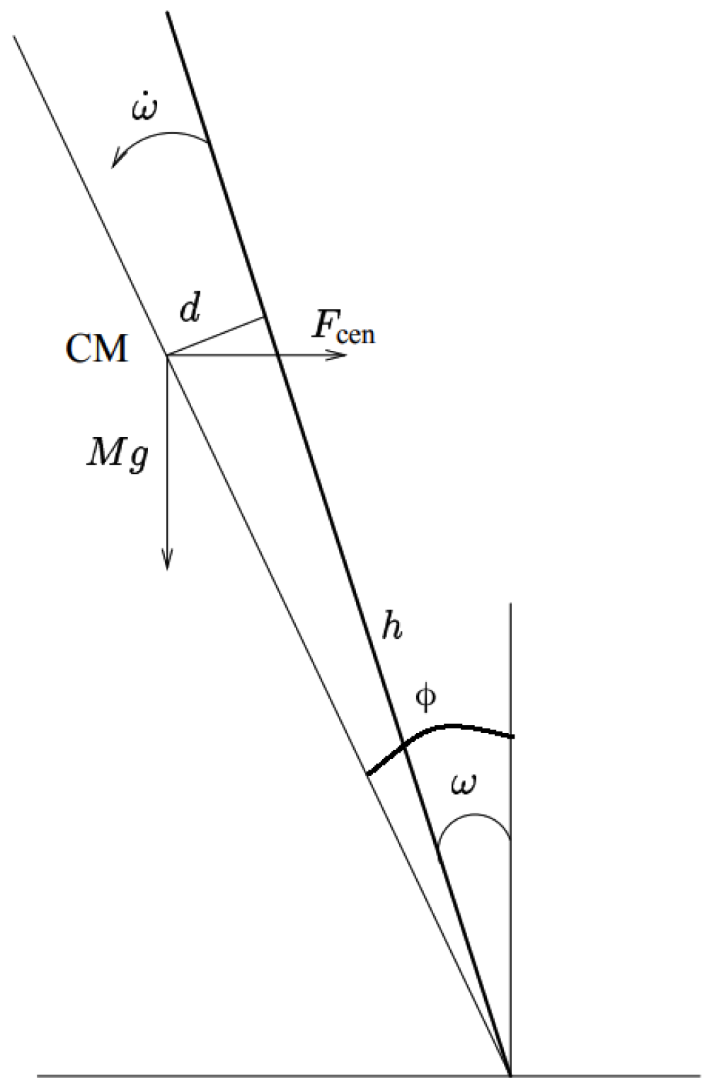
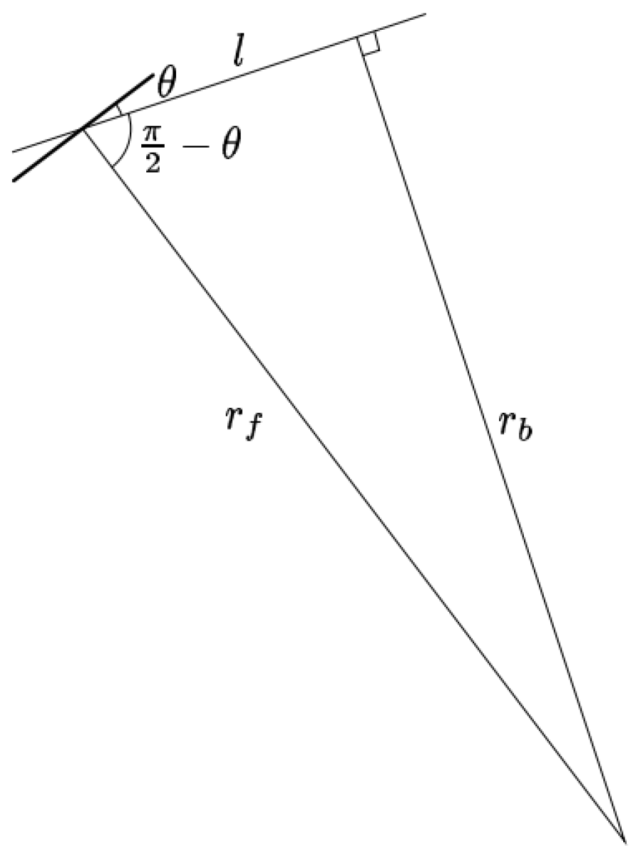
3. Extended Bicycle Dynamics

Studies on bicycle dynamics are often studied by researchers [2,5,9,17]. The first bicycle studied by Randlov [9] is illustrated in Figure 1.
This paper not only utilizes the work of Randlov [9] study, but also extends it to where the velocity of the bicycle is dynamic. Particularly, the bicycle has six dimensional states: ( ω , ω ˙ , ω ¨ , θ , θ ˙ , ψ g ) where ω , ω ˙ , ω ¨ are the angle, angular velocity, and angular acceleration of the bicycle relative to the vertical plane. θ , θ ˙ are the angle and angular velocity of the handlebars and ψ g is the angle formed by the bicycle and a specified goal g. The bicycle states are demonstrated in Figure 2. To control the bicycle, the agent chooses three actions. The first action is the torque applied to the handlebar (T). The second action is the displacement (d) between the center of mass and the bicycle plan (Figure 3). The third action is the force (F) applied to the pedal of the bicycle.
The equations of the position of the tires for the front tire:
x f y f ( t + 1 ) = x f y f ( t ) + v d t sin ψ + θ + s i g n ( ψ + θ ) arcsin ( v d t 2 r f ) cos ψ + θ + s i g n ( ψ + θ ) arcsin ( v d t 2 r f ) ,
and for the back tire:
x b y b ( t + 1 ) = x b y b ( t ) + v d t sin ψ + s i g n ( ψ ) arcsin ( v d t 2 r b ) cos ψ + s i g n ( ψ ) arcsin ( v d t 2 r b ) ,
where ψ is angle make by bicycle and horizontal line, and r b and r f (Figure 4) are radii of the front tire and back tire, respectively. The radii are given by:
r f = l | cos ( π 2 θ ) | = l | sin θ | .
and
r b = l | tan π 2 θ | = l | tan θ |
The angular acceleration ω ¨ can be calculated as:
ω ¨ = 1 I b i c y c l e M h g sin ϕ cos ϕ I d c σ ˙ θ ˙ + s i g n ( θ ) v 2 M d r r f + M d r r b + M h r C M ,
where angle ϕ is the total angle of tilt of the center of mass (CM) (Figure 3), and is defined as:
ϕ = ω + a r c t a n ( d h ) .
The angular acceleration θ ¨ of the front tire and the handle bar is
θ ¨ = T I d v σ ˙ ω ˙ I d l .
The moment of inertia has the formula:
I b i c y c l e = 13 3 M c h 2 + M p ( h + d C M ) 2 ,
where various moments of inertia for a tire (Figure 5) are estimated to: I d c = M d r 2 , I d v = 3 2 M d r 2 , I d l = 1 2 M d r 2 .
The velocity of the bicycle can be adjusted by learning the force applied to the pedal. Figure 6 shows how the force applied to the pedal can be transmitted to the bicycle. Using the static equilibrium assumption, we can write the following torque equations:
F 1 R 1 = F 2 R 2
and
F 3 R 3 = F 4 R 4 .
Since F 2 = F 3 , we can combine the above two equations to give an expression for F 4 :
F 4 = F 1 R 1 R 3 R 2 R 4 .
The force F 4 determines the acceleration of the bicycle. Particularly, the acceleration of the bicycle is as follows:
a = F 4 M c + M d + M p .
From the acceleration, we can calculate the velocity of the bicycle:
v = v + Δ t × a .
Various parameters for the bicycle dynamics are shown in Table 1.

4. Method to Control Bicycle

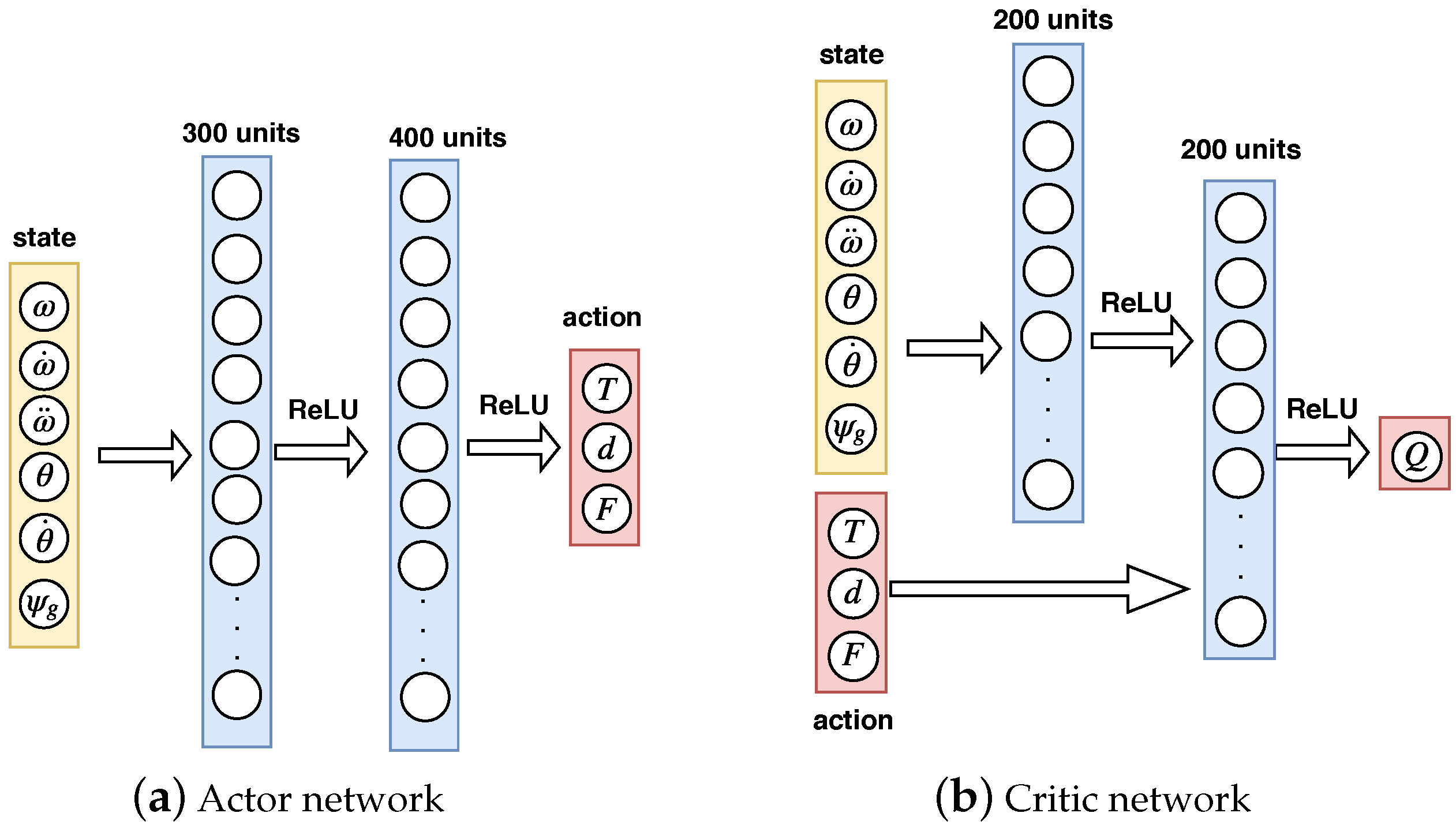
4.1. Network Structure

There are two networks used for training, namely a critic network and an actor network, which are illustrated in Figure 7. The input of the actor network is a 6-dimensional state vector and the output of the actor network is a 3-dimensional action vector. Meanwhile, the input of the critic network is both a state vector and an action vector, and the output of the critic network is a Q action value. The configurations of the actor network and critic network are shown in Table 2. Two hidden layers of the actor network have 300 units and 400 units, respectively, while both hidden layers of the critic network have 200 units. The action vector only joins the network at the second hidden layers. The parameters of the networks are initialized randomly and are optimized using the ADAM algorithm [18]. The target networks are updated using a soft-updating technique with learning rate τ = 0.001 . We did not try different numbers of layers of units. From our experience, however, neural networks are quite flexible and can cope with a variety of settings.

4.2. Network Training

Critic network training. Critic networks include a main critic network (Q) parameterized by θ Q and a target critic network ( Q ) parameterized by θ Q . At every discrete time step, the main network is updated using a batch of samples, which obtains data from the replay memory. Particularly, θ Q is optimized to minimize the loss function as follows:
L = 1 N i y i Q s i , a i | θ Q 2 ,
where i indicates the ith sample in the batch and
y i = r i + γ Q s t + 1 , μ s t + 1 | θ μ | θ Q .
θ Q is coupled with θ Q using a soft-updating technique with learning rate τ as follows:
θ Q τ θ Q + ( 1 τ ) θ Q .
Actor network training. Similarly, actor networks include a main actor network ( μ ) parameterized by θ μ and a target actor network ( μ ) parameterized by θ μ . The main actor network is updated using the deterministic policy gradient theorem [15] as follows:
θ μ μ | s i 1 N i a Q s , a | θ Q | s = s i , a = μ s i × θ μ μ s | θ μ | s i ,
where a Q is the gradient of the critic w.r.t. action a and θ μ μ is the gradient of actor w.r.t. parameter θ μ . θ μ is updated using a soft-updating technique with learning rate τ as follows:
θ μ τ θ μ + ( 1 τ ) θ μ .

4.3. Learning Process

Applying reinforcement learning to the bicycle problem is described as follows. The state of a bicycle includes ( ω , ω ˙ , ω ¨ , θ , θ ˙ , ψ g ), where ω , ω ˙ , ω ¨ are the angle, angular velocity, and angular acceleration of the bicycle relative to the vertical plane; θ , θ ˙ are the angle and angular velocity of the handlebars and ψ g is the angle formed by the bicycle and a specified goal g. These states are sent to the controller at each time step and the controller returns the values of d, the torque T, and the force F applied to the pedal.
How the DDPG algorithm trains the controller is summarized in Figure 8. Let Q ( s , a | θ Q ) and Q ( s , a | θ Q ) be the main network and target network of the critic, respectively, μ ( s , a | θ μ ) and μ ( s , a | θ μ ) be the main network and the target network of the actor, respectively, and R be the experience replay. The learning process is described as follows:
(1) The agent observes state s t from the bicycle and feeds it to the actor network (step [1] in Figure 8) for estimating the next action a t (step [2] in Figure 8) as follows:
a t = μ s t | θ μ + N t ,
where N t is small random noise for exploring the action space.
(2) The bicycle transits to next state s t + 1 and returns reward r t to the agent.
(3) The sampled data s t , a t , r t , s t + 1 is then stored the experience replay for later use (step [3] in Figure 8).
(4) From the experience replay memory, we randomly select a batch of N samples and use them to train the networks (step [4] in Figure 8).
(5) Train the critic network (step [5] and step [6] in Figure 8) by minimizing the loss function as Equation (14).
(6) Train the actor network (step [7] in Figure 8) using the deterministic policy gradient as Equation (17).
(7) Thereafter, the parameters of the target networks ( θ μ and θ Q ) are updated using soft-update techniques as Equations (16) and (18).

4.4. Reward Function

The reward function is defined as follows:
r ( s , a ) = the last reward before falling down ω > π 6 ( ω 2 + 0.1 ω ˙ 2 + 0.01 ω ¨ 2 ) 2.0 ψ g 2 ω < π 6 ,
where the term ( ω 2 + 0.1 ω ˙ 2 + 0.01 ω ¨ 2 ) takes responsibility for balancing the bicycle and the term 2 ψ g 2 is for leading the bicycle to the goal. In this reward function, the bicycle is considered as falling down if the angle between the bicycle and the vertical plane is greater than π 6 rad (or 30 degree). When the bicycle falls down, the reward at this time is used until the end of the episode. The coefficients for each term are selected based on their contributions to the reward. Particularly, we use a coefficient of 1.0 for ω 2 , which is the most important in the balancing term. A coefficient of 2.0 is used for ψ g to highlight the importance of the go-to-goal term. Figure 9 shows the effects of the components on the reward value. Initially, the term 2 ψ g 2 has a small value compared to ω 2 , 0.1 ω ˙ 2 and 0.01 ω ¨ 2 . This indicates that this term is the most important to the reward function. However, during 5000 training episodes, the gap between the 2 ψ g 2 term and the other terms is decreases and all terms are tend to zero.

5. Experiments

5.1. Settings

The simmlation environment is as follows. The operating system is Linux (Ubuntu 16.04 LTS) with 64 GB DDR3 memory. We use PyCharm as an integrated development environment and experiment with Python as a language. Parameters of the algorithm are shown in Table 3, where we use the Ornstein-Uhlenbeck process [19] to explore the action space. The experience replay can contain up to 500,000 data samples. At each training step, we randomly obtain a batch of 64 samples from the experience replay and use them to train the controller.

5.2. Baselines

NAF (Normalized Advantage Function) [20] uses a Q neural network for the entire problem. To adapt to the continuous control tasks, the Q network is decomposed into a state value term V and an advantage term A:
Q ( s , a | θ Q ) = A ( s , a | θ A ) + V ( s | θ V )
The advantage A is parameterized as a quadratic function of nonlinear features of the state:
A ( s , a | θ A ) = 1 2 ( a μ ( s | θ μ ) ) T P ( s | θ P ) ( a μ ( s | θ μ ) ) .
P ( s | θ P ) is a square matrix with formula:
P ( s | θ P ) = L ( s | θ P ) L ( s | θ P ) T
where L ( s | θ P ) is a lower-triangular matrix with entries come from a linear output layer of a neural network. This representation of the Q-network can deal with continuous action tasks.
PPO (Proximal Policy Optimization) [21] is an on-policy algorithm. This means that the policy is learned from the trajectories that are generated from current policy instead of the trajectories from the replay memory. PPO gets rid of the computation created by constrained optimization. PPO implements the idea of TRPO’s constraint [22], which does not allow the policy to change too much but instead uses a simpler form of equation. The features of this algorithm can be summarized as follows. First, denote the probability ratio between the old and new policies as
r ( θ ) = π θ ( a | s ) π θ o l d ( a | s ) .
PPO imposes the constraint by forcing r ( θ ) to stay within a small interval around 1, precisely [1 − ϵ , 1 + ϵ ], where ϵ is a hyperparameter.
J C L I P ( θ ) = E m i n ( r ( θ ) A ^ θ o l d ( s , a ) , c l i p ( r ( θ ) , 1 ϵ , 1 + ϵ ) A ^ θ o l d ( s , a ) )
The function clip ( r ( θ ) , 1 ϵ , 1 + ϵ ) clips the ratio within [ 1 ϵ , 1 + ϵ ]. The objective function of PPO uses the minimum value between the original value and the clipped version, and therefore we lose the motivation for increasing the policy update to extremes to obtain better rewards.
When applying PPO to the network architecture with shared parameters for both the policy (actor) and value (critic) functions, in addition to the clipped reward, the objective function is augmented with an error term in the estimation (the second term in the formula) and an entropy term (the third term in the formula) to encourage sufficient exploration.
J C L I P ( θ ) = E [ J C L I P ( θ ) c 1 ( V θ ( s ) V t a r g e t ) 2 + c 2 H ( s , π θ ( . ) ) ]
Here, both c 1 and c 2 are hyperparameter constants.

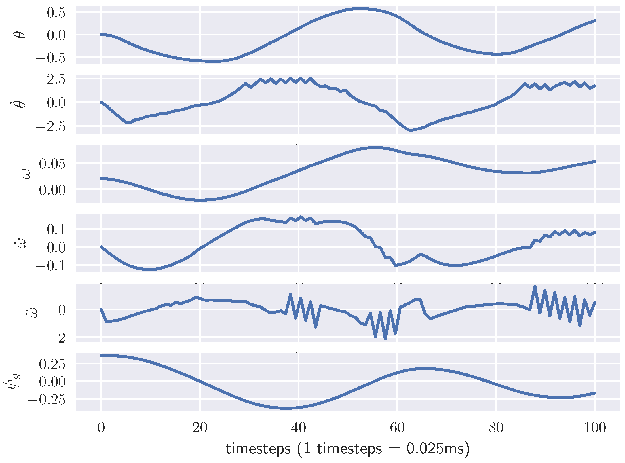
5.3. Results and Discussion

In this section, we compare the performance of a controller-based DDPG with other baselines. In addition, we show the performance of the bicycle before and after considering the velocity. The results are shown below.

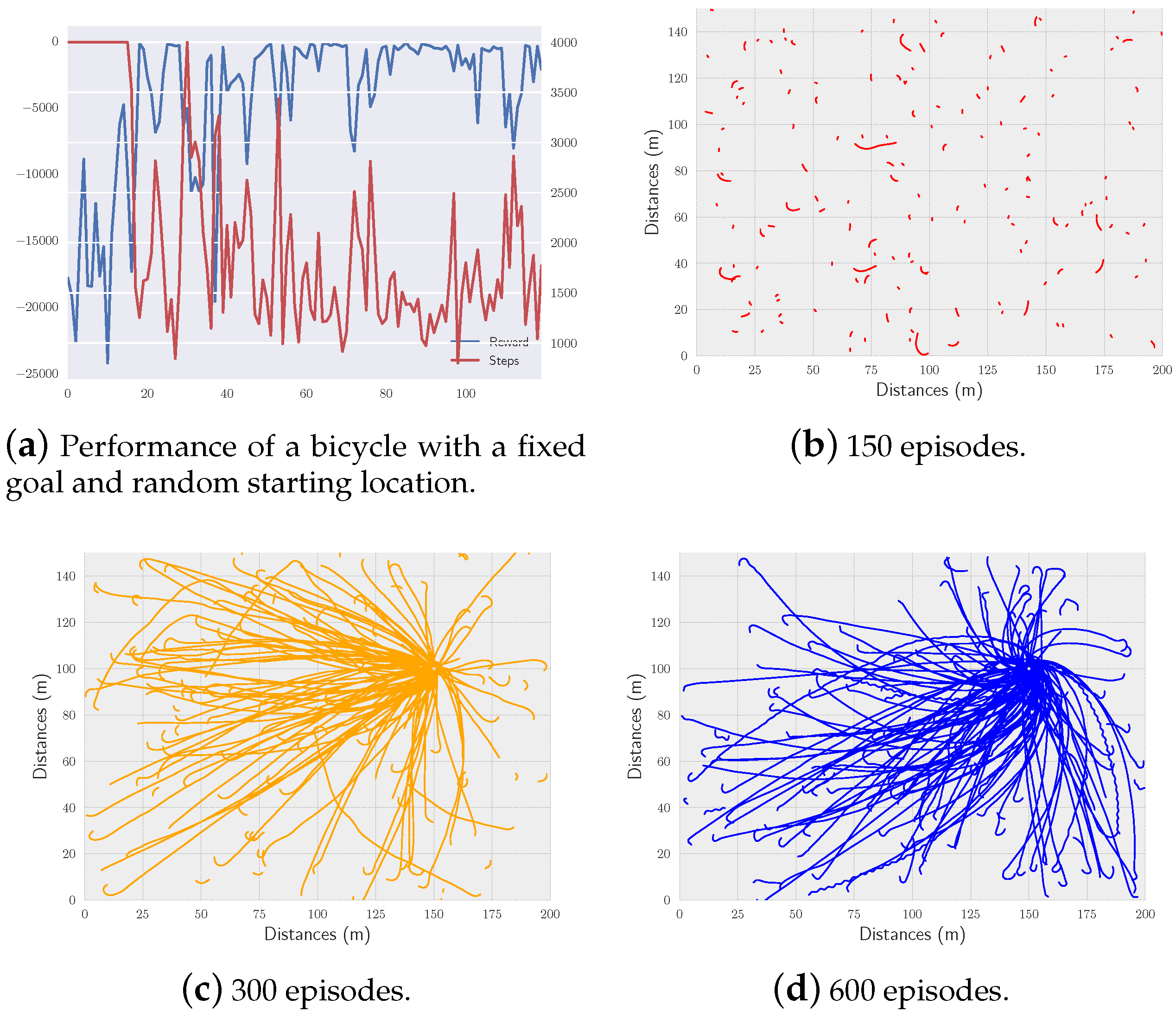
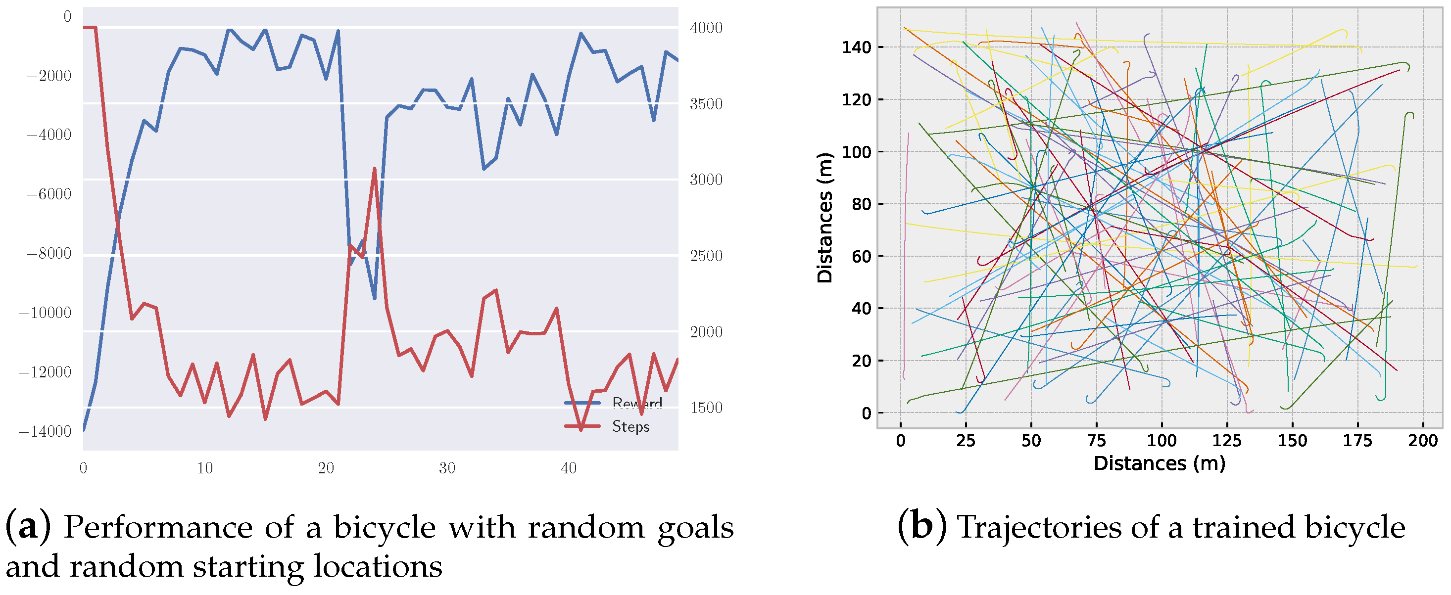
5.3.1. Simulation without Controlling the Velocity

Comparison with baselines. In the first evaluation, we compare the performance of a bicycle trained by DDPG algorithms with the performance of the bicycle trained by other algorithms. Particularly, we compare DDPG with the NAF algorithm (Normalized Advantage Function algorithm) and PPO algorithm (Proximal Policy Optimization algorithm). Both algorithms are state-of-the-art deep reinforcement learning algorithms that can deal with a highly continuous action space. Both algorithms produce deterministic policies that are expected to have lower variance and predictable performance compared to a stochastic policy. Figure 10 shows the performance of a bicycle that randomly starts at ( 50 , 50 ) m and wants to reach a goal at ( 60 , 65 ) m. The speed of the bicycle is fixed at 10 km/h and the displacement d is in the range from −20 cm to 20 cm. We report the performance throughout three runs of 5000 episodes. Each episode has 400 time steps.
From the figure, we can see that the controller trained by DDPG outperforms the controller trained by other algorithms in term of variance and reward values. At the beginning of the learning process, DDPG seems to has a bigger variance than other algorithms. However, at the end of the learning process, the variance of DDPG algorithm is decreased while the variance of PPO algorithm is increased and bigger than other algorithms. The algorithm PPO (under development) is expected to gradually train a stable controller but not better than the DDPG algorithm on bicycle domain. The difficulty in tuning PPO’s hyperparameters might be the reason for the reported results. In addition, PPO takes a long time to obtain the same performance as DDPG. Even though NAF can learn something on bicycle controller, it cannot obtain a good controller for stabilizing the bicycle. Figure 11 shows values of 6-dimensional states of a successful trajectory. The figure shows that all of states are stable and gradually converges to zero.
Fixed start-fixed goal. The second evaluation shows the performance of a bicycle with different values of d. The bicycle randomly starts at ( 50 , 50 ) m with a random direction and wants to reach a goal at ( 60 , 65 ) m. The speed is fixed at 10 km/h. We train for 5000 episodes of 400 time steps. We learn for 5000 episodes of 400 time steps. The result reported in Figure 12a shows that an agent using a big displacement to adjust the center of mass will outperform an agent using a small displacement and an agent without displacement (only steering the handlebar). Intuitively, without considering d, the bicycle will easily fall down when it tries to turn the bicycle at a high speed. Figure 12 shows the trajectories of the back wheel of the bicycle during the learning process. During this time, the bicycle gradually reaches the goal (blue lines are early trajectories and red lines are late trajectories). However, the bicycle that starts at the opposite position of the goal location often falls down.
Random start-fixed goal. The next evaluation is performed for a bicycle that starts at a random location and learns to reach a goal position at ( 150 , 100 ) m. After around 700 episodes, the bicycle almost reaches the goal from any staring location. The reward converges to zero and the average number of steps to reach decreases from the initial steps (4000) to around 1000 (Figure 13a). Figure 13 shows the trajectories of the bicycle during the learning process.
Random start-random goal. In the last evaluation of this section, we report the performance of a bicycle controller that is trained to start at random locations and reach a random goal. Figure 14a shows the same behaviors as the previous evaluations. This means the average cumulative reward converges to zero and the average number of steps decreases. Figure 14b shows 100 trajectories for a trained bicycle that starts at random locations and reaches pre-defined random goals. In all of the cases, the bicycle reaches the goal.

5.3.2. Simulation with Controlling the Velocity

Learning to turn. Understanding the force applied to the pedal is necessary to adjust the velocity of the bicycle. This evaluation shows the efficiency of the controller that learns the force applied to pedal simultaneously. The bicycle in this evaluation only uses a small displacement (from −2 cm to 2 cm) and randomly starts at a position that is in the opposite direction of the goal at ( 60 , 65 ) m. We compare the performances between a controller that learns the velocity and a controller that does not. The performance is reported through 10,000 episodes of 500 steps each. The initial velocity is 2.5 m/s. Figure 15a shows the average reward, while Figure 15b,c show the trajectories of the bicycle during the learning process. From the figure, we can see that learning a pedal’s force helps the bicycle turn the wheel when the bicycle is facing the opposite direction from the goal. The way a bicycle turns the wheel by adjusting the pedal’s force is shown in Figure 15d. If the bicycle is facing the opposite direction from the goal’s location, the bicycle will adjust the pedal’s force to reduce the speed. Under this low speed, the bicycle can easily turn. After the bicycle turns to face direction of the goal’s location, the bicycle increases the speed to get to the goal as soon as possible. In the case the bicycle already faces the direction as the goal’s location, the bicycle simply gradually increases the speed and heads toward to the goal.
Random start-random goal-learned velocity. In the final evaluation, we increase the complexity of the domain’s state space by allowing the bicycle to start at any location with any direction and requiring it reach to a random location. The speed of the bicycle ranges from 1 m/s to 5 m/s and is adjusted by the force applied to the pedal, which ranges from 100 N to 100 N. The initial speed of the bicycle is 2 m/s. We average the performance of the controller after three runs of 10,000 episodes. The report shown in Figure 16 indicates that the controller is gradually improved by increasing the average reward and decreasing average step and distance to the goal. The speed of the bicycle is decreased to 2 m/s in the first 100 steps and then increases a little before being stabilizing at around 2 m/s. Intuitively, the trained controller decreases the velocity to help the bicycle become stable when turning time. However, due to the curve of dimensionality, the controller needs to explore more of the state space and action space, requiring training via a millions of episodes to obtain an optimal controller.

6. Conclusions and Future Works

In this paper, we propose a method to control a bicycle using the DDPG algorithm and show that it can be successfully controlled. A controller with a deep neural network can rotate the bicycle handlebars, move the center of gravity displacement, and adjust the speed so that the bicycle can change directions without collapsing. The agent using the proposed neural network controller in this paper was able to reach a specified position and generate a gentle and smooth trajectory. For future work, first, we can enhance the controller by forcing the bicycle to follow a pre-defined trajectory such as a bicycle running on the road. In addition, the DDPG algorithm requires picking a step size that falls into the right range. If it is too small, the training progress will be extremely slow. If it is too large, training tends to be overwhelmed by noise, leading to poor performance. The DDPG algorithm does not assure monotonically improved performance of the controller. Therefore, the second future work is using PPO with some modifications to obtain a more stable controller. Finally, making a real autonomous bicycle needs to consider many aspects such as the effect of a cyclist on the handlebar (T), the effect of the cyclist’s foot on the force to pedal, or the hardware needed to build the bicycle. However, most of them have been ignored in this study for simplifying the learning problem. A study on these aspects will be valuable to make a full understanding of an autonomous bicycle.

Author Contributions

Conceptualization, S.L. and T.C.; methodology, S.C. and T.P.L.; software, S.C. and T.P.L.; validation, Q.D.N. and M.A.L.; formal analysis, S.L. and T.C.; investigation, S.L. and T.C.; resources, T.P.L.

Funding

The authors are grateful to the Basic Science Research Program through the National Research Foundation of Korea (NRF-2017R1D1A1B04036354).

Conflicts of Interest

The authors declare no conflict of interest.

References

  1. Nederland, G. Introducing the self-driving bicycle in The Netherlands. Available online: https://www.youtube.com/watch?v=LSZPNwZex9s (accessed on 10 December 2018).
  2. Keo, L.; Yamakita, M. Controlling balancer and steering for bicycle stabilization. In Proceedings of the IEEE/RSJ International Conference on Intelligent Robots and Systems, St. Louis, MO, USA, 10–15 October 2009; pp. 4541–4546. [Google Scholar]
  3. Meijaard, J.P.; Papadopoulos, J.M.; Ruina, A.; Schwab, A.L. Linearized dynamics equations for the balance and steer of a bicycle: a benchmark and review. In Proceedings of the Royal Society of London A: Mathematical, Physical and Engineering Sciences; The Royal Society: London, UK, 2007; Volume 463, pp. 1955–1982. [Google Scholar]
  4. Schwab, A.; Meijaard, J.; Kooijman, J. Some recent developments in bicycle dynamics. In Proceedings of the 12th World Congress in Mechanism and Machine Science; Russian Academy of Sciences: Moscow, Russia, 2007. [Google Scholar]
  5. Tan, J.; Gu, Y.; Liu, C.K.; Turk, G. Learning bicycle stunts. ACM Trans. Gr. (TOG) 2014, 33, 50. [Google Scholar] [CrossRef]
  6. Lu, M.; Li, X. Deep reinforcement learning policy in Hex game system. In Proceedings of the IEEE Chinese Control And Decision Conference (CCDC), Shenyang, China, 9–11 June 2018; pp. 6623–6626. [Google Scholar]
  7. Bejar, E.; Moran, A. Deep reinforcement learning based neuro-control for a two-dimensional magnetic positioning system. In Proceedings of the IEEE 4th International Conference on Control, Automation and Robotics (ICCAR), Auckland, New Zealand, 20–23 April 2018; pp. 268–273. [Google Scholar]
  8. Yasuda, T.; Ohkura, K. Collective behavior acquisition of real robotic swarms using deep reinforcement learning. In Proceedings of the Second IEEE International Conference on Robotic Computing (IRC), Laguna Hills, CA, USA, 31 January–2 February 2018; pp. 179–180. [Google Scholar]
  9. Randløv, J.; Alstrøm, P. Learning to drive a bicycle using reinforcement learning and shaping. ICML 1998, 98, 463–471. [Google Scholar]
  10. Le, T.P.; Chung, T.C. Controlling bicycle using deep deterministic policy gradient algorithm. In Proceedings of the 14th International Conference on Ubiquitous Robots and Ambient Intelligence (URAI), Jeju, Korea, 28 June–1 July 2017; pp. 413–417. [Google Scholar]
  11. Sutton, R.; Barto, A. Reinforcement Learning: An Introduction; MIT Press: Cambridge, MA, USA, 1998; Volume 1. [Google Scholar]
  12. Peters, J.; Schaal, S. Reinforcement learning of motor skills with policy gradients. Neural Netw. 2008, 21, 682–697. [Google Scholar] [CrossRef] [PubMed] [Green Version]
  13. Lillicrap, T.P.; Hunt, J.J.; Pritzel, A.; Heess, N.; Erez, T.; Tassa, Y.; Silver, D.; Wierstra, D. Continuous control with deep reinforcement learning. arXiv, 2015; arXiv:1509.02971. [Google Scholar]
  14. Le, T.P.; Quang, N.D.; Choi, S.; Chung, T. Learning a self-driving bicycle using deep deterministic policy Gradient. In Proceedings of the 18th International Conference on Control, Automation and Systems (ICCAS), Pyeongchang, Korea, 17–20 October 2018; pp. 231–236. [Google Scholar]
  15. Silver, D.; Lever, G.; Heess, N.; Degris, T.; Wierstra, D.; Riedmiller, M. Deterministic policy gradient algorithms. In Proceedings of the 31st International Conference on Machine Learning, Beijing, China, 21–26 June 2014; pp. 387–395. [Google Scholar]
  16. Mnih, V.; Kavukcuoglu, K.; Silver, D.; Rusu, A.A.; Veness, J.; Bellemare, M.G.; Graves, A.; Riedmiller, M.; Fidjeland, A.K.; Ostrovski, G.; et al. Human-level control through deep reinforcement learning. Nature 2015, 518, 529. [Google Scholar] [CrossRef] [PubMed]
  17. Hwang, C.L.; Wu, H.M.; Shih, C.L. Fuzzy sliding-mode underactuated control for autonomous dynamic balance of an electrical bicycle. IEEE Trans. Control Syst. Technol. 2009, 17, 658–670. [Google Scholar] [CrossRef]
  18. Kingma, D.P.; Ba, J. Adam: A method for stochastic optimization. arXiv, 2014; arXiv:1412.6980. [Google Scholar]
  19. Uhlenbeck, G.E.; Ornstein, L.S. On the theory of the Brownian motion. Phys. Rev. 1930, 36, 823. [Google Scholar] [CrossRef]
  20. Gu, S.; Lillicrap, T.; Sutskever, I.; Levine, S. Continuous deep q-learning with model-based acceleration. In Proceedings of the International Conference on Machine Learning, New York, NY, USA, 19–24 June 2016; pp. 2829–2838. [Google Scholar]
  21. Schulman, J.; Wolski, F.; Dhariwal, P.; Radford, A.; Klimov, O. Proximal policy optimization algorithms. arXiv, 2017; arXiv:1707.06347. [Google Scholar]
  22. Schulman, J.; Levine, S.; Abbeel, P.; Jordan, M.; Moritz, P. Trust region policy optimization. In Proceedings of the International Conference on Machine Learning, Lille, France, 6–11 July 2015; pp. 1889–1897. [Google Scholar]
Figure 1. Illustration of a bicycle.
Symmetry 11 00290 g001
Figure 2. Demonstration of 6-dimensional states.
Symmetry 11 00290 g002
Figure 3. The bicycle seen from behind. The thick line represents the bicycle [9].
Symmetry 11 00290 g003
Figure 4. The bicycle seen from above. The thick line represents the front tire [9].
Symmetry 11 00290 g004
Figure 5. Axis for the moments of inertia for a tire [9].
Symmetry 11 00290 g005
Figure 6. Force transmission from the pedal.
Symmetry 11 00290 g006
Figure 7. The two neural networks used in this paper.
Symmetry 11 00290 g007
Figure 8. Workflow of the deep deterministic policy gradient (DDPG) algorithm applied to the bicycle.
Symmetry 11 00290 g008
Figure 9. Contributions of the components to the reward function.
Symmetry 11 00290 g009
Figure 10. Performance comparison of DDPG with baselines algorithms.
Symmetry 11 00290 g010
Figure 11. Observed states of a successful trajectory.
Symmetry 11 00290 g011
Figure 12. Trajectory of a bicycle starting at (50, 50) m and reaching the goal at (60, 65) m.
Symmetry 11 00290 g012
Figure 13. Bicycle trajectories during learning.
Symmetry 11 00290 g013
Figure 14. Bicycle with random goal locations and random starting locations.
Symmetry 11 00290 g014
Figure 15. A bicycle learning to turn.
Symmetry 11 00290 g015
Figure 16. The performance of a bicycle starting at any place to reach a random location.
Symmetry 11 00290 g016
Table 1. Parameters of bicycle dynamics [9].
NotationDescriptionValue
cHorizontal distance between the point,
where the front wheel touches the ground and the CM
66 cm
C M The Center of Mass of the bicycle and cyclist as a whole
dThe agent’s choice of the displacement of the CM
perpendicular to the plane of the bicycle
d C M The vertical distance between the CM for
the bicycle and for the cyclist
30 cm
hHeight of the CM over the ground94 cm
lDistance between the front tire and the back tyre
at the point where they touch the ground
111 cm
M c Mass of the bicycle15 kg
M d Mass of a tire1.7 kg
M p Mass of the cyclist60 kg
rRadius of the tire34 cm
σ ˙ The angular velocity of a tire σ ˙ = v r
TThe torque the agent applies to the handlebars
d t Time step0.025 s
Table 2. Parameters of the actor network and the critic network.
NameActorCritic
Input layerA state vector ( s t )State vector and action vector ( s t , a t )
1st fully-connected layer400 units200 units
2nd fully-connected layer300 units200 units
Output layerAn action vector ( a t )Q-value
Initial parametersUniformly random between
3 e 3 , 3 e 3
Uniformly random between
3 e 3 , 3 e 3
Learning rate0.0010.001
OptimizerADAM [18]ADAM [18]
Table 3. Parameters of algorithm.
NameValue
Input dimension6 (states)
Output dimension3 (actions)
Discounted factor0.99
Random noiseOrnstein-Uhlenbeck process [19] with θ = 0.15 and σ = 0.2
Experience memory capacity500,000
Batch size64 samples

