Some Real-Life Applications of a Newly Constructed Derivative Free Iterative Scheme

Abstract

In this study, we present a new higher-order scheme without memory for simple zeros which has two major advantages. The first one is that each member of our scheme is derivative free and the second one is that the present scheme is capable of producing many new optimal family of eighth-order methods from every 4-order optimal derivative free scheme (available in the literature) whose first substep employs a Steffensen or a Steffensen-like method. In addition, the theoretical and computational properties of the present scheme are fully investigated along with the main theorem, which demonstrates the convergence order and asymptotic error constant. Moreover, the effectiveness of our scheme is tested on several real-life problems like Van der Waal’s, fractional transformation in a chemical reactor, chemical engineering, adiabatic flame temperature, etc. In comparison with the existing robust techniques, the iterative methods in the new family perform better in the considered test examples. The study of dynamics on the proposed iterative methods also confirms this fact via basins of attraction applied to a number of test functions.

1. Introduction

In the last few years, several scholars introduced the concept of how to remove derivatives from the iteration functions. The main practical difficulty associated with iterative methods involving derivatives is to calculate first and/or high-order derivatives at each step, which is quite difficult and time-consuming. Computing derivatives of standard nonlinear equations (which are generally considered for academic purposes) is an easy task. On the other hand, in regard to practical problems of calculating the derivatives of functions, it is either very expensive or requires a huge amount of time. Therefore, we need derivative free methods, software or tools which are capable of generating derivatives automatically (for a detailed explanation, please see [1]).

There is no doubt that optimal 8-order multi-point derivative free methods are one of the important classes of iterative methods. They have faster convergence towards the required root and a better efficiency index as compared to Newton/Steffensen’s method. In addition, one can easily attain the desired accuracy of any specific number of digits within a small number of iterations with the help of these iterative methods.

In recent years, many scholars have proposed a big number of 8-order derivative free schemes in their research articles [2,3,4,5,6,7,8,9,10,11,12,13,14,15,16,17,18]. However, most of these eighth-order methods are the extensions or modifications of particularly well-known or unknown existing optimal fourth-order derivative free methods; for detailed explanations, please see [5,6,14,16,17]. However, there is no optimal derivative free scheme in a general way that is capable of producing optimal eighth-order convergence from every optimal fourth-order derivative free scheme to date, according to our knowledge.

In this paper, we present a new optimal scheme that doesn’t require any derivative. In addition, the proposed scheme is capable of generating new optimal 8-order methods from the earlier optimal fourth-order schemes whose first substep employs Steffensen’s or a Steffensen-type method. In this way, our scheme is giving the flexibility in the choice of a second-step to the scholars who can pick any existing optimal derivative free fourth-order method (available in the literature) unlike the earlier studies. The construction of the presented scheme is based on a technique similar to Sharma et al. [19] along with some modifications that can be seen in the next section. We tested the applicability of a newly proposed scheme on a good variety of numerical examples. The obtained results confirm that our methods are more efficient and faster as compared to existing methods in terms of minimum residual error, least asymptotic error constants, minimum error between two consecutive iterations, etc. Moreover, we investigate their dynamic behavior in the complex plane adopting basins of attraction. Dynamic behavior provides knowledge about convergence, and stability of the mentioned methods also supports the theoretical aspects.

2. Construction of the Proposed Scheme

This section is devoted to 8-order derivative free schemes for nonlinear equations. In order to obtain this scheme, we consider a general fourth-order method $\eta (v_j,x_j,y_j)$ in the following way:

$$\left\{\begin{array}{cc}\hfill y_j& =x_j-\frac{f\left(x_j\right)}{f[v_j,x_j]},\hfill \\ \hfill z_j& =\eta (v_j,x_j,y_j),\hfill \end{array}\right.$$

(1)

where $v_j=x_j+\lambda f\left(x_j\right),\lambda \in \mathbb{R}$ and $f[v_j,x_j]=\frac{f\left(v_j\right)-f\left(x_j\right)}{v_j-x_j}$ are the first-order finite difference. We can simply obtain eighth-order convergence by applying the classical Newton’s technique, which is given by

$$\begin{array}{cc}\hfill x_{j+1}=& z_j-\frac{f\left(z_j\right)}{f^{\prime }\left(z_j\right)}.\hfill \end{array}$$

(2)

The above scheme is non optimal because it does not satisfy the Kung–Traub conjecture [7]. Thus, we have to reduce the number of evaluations of functions or their derivatives. In this regard, we some approximation of the first-order derivative For this purpose, we need a suitable approximation approach of functions that can approximate the derivatives. Therefore, we choose the following rational functional approach

$$\Omega \left(x\right)=\Omega \left(x_j\right)-\frac{(x-x_j)+{\theta }_1}{{\theta }_2{(x-x_j)}^2+{\theta }_3(x-x_j)+{\theta }_4},$$

(3)

where ${\theta }_i,i=1,2,3,4$ are free parameters. This approach is similar to Sharma et al. [19] along with some modifications. We can determine these disposable parameters ${\theta }_i$ by adopting the following tangency constraints

$$\Omega \left(x_j\right)=f\left(x_j\right),\Omega \left(v_j\right)=f\left(v_j\right),\Omega \left(y_j\right)=f\left(y_j\right),\Omega \left(z_j\right)=f\left(z_j\right).$$

(4)

The number of tangency conditions depends on the number of undetermined parameters. If we increase the number of undetermined parameters in the above rational function, then we can also attain high-order convergence (for the detailed explanation, please see Jarratt and Nudds [20]).

By imposing the first tangency condition, we have

$${\theta }_1=0.$$

(5)

The last three tangency conditions provide us with the following three linear equations:

$$\begin{array}{c}{\theta }_2{(v_j-x_j)}^2+{\theta }_3(v_j-x_j)+{\theta }_4=\frac{1}{f[v_j,x_j]},\hfill \\ {\theta }_2{(y_j-x_j)}^2+{\theta }_3(y_j-x_j)+{\theta }_4=\frac{1}{f[y_j,x_j]},\hfill \\ {\theta }_2{(z_j-x_j)}^2+{\theta }_3(z_j-x_j)+{\theta }_4=\frac{1}{f[z_j,x_j]},\hfill \end{array}$$

(6)

with three unknowns ${\theta }_2,{\theta }_3$ and ${\theta }_4$.

After some simplification, we further yield

$$\begin{array}{cc}\hfill {\theta }_2& =\frac{f\left(v_j\right)+{\theta }_{4}f[x_j,v_j]f[x_j,y_j](y_j-v_j)-f\left(y_j\right)}{(f\left(v_j\right)-f\left(x_j\right))(f\left(x_j\right)-f\left(y_j\right))(v_j-y_j)},\hfill \\ \hfill {\theta }_3& =-\frac{{\theta }_2(f\left(v_j\right)-f\left(x_j\right))(v_j-x_j)+{\theta }_{4}f[x_j,v_j]-1}{f\left(v_j\right)-f\left(x_j\right)},\hfill \\ \hfill {\theta }_4& =\frac{(f\left(x_j\right)-f\left(y_j\right))(f\left(x_j\right)-f\left(z_j\right))(y_j-z_j)-a}{f[x_j,v_j]f[x_j,y_j]f[x_j,z_j](v_j-y_j)(v_j-z_j)(y_j-z_j)},\hfill \end{array}$$

(7)

where $a=(f\left(v_j\right)-f\left(x_j\right))[(f\left(x_j\right)-f\left(y_j\right))(v_j-y_j)+(f\left(z_j\right)-f\left(x_j\right))(v_j-z_j)]$ and $f[·,·]$ are the finite difference of first order. Now, we differentiate the expression (3) with respect to x at the point $x=z_j$, which further provides

$$f^{\prime }\left(z_j\right)\approx {\Omega }^{\prime }\left(z_j\right)=\frac{{\theta }_4-{\theta }_2{(z_j-x_j)}^2}{{\left[{\theta }_2{(z_j-x_j)}^2+{\theta }_3(z_j-x_j)+{\theta }_4\right]}^2}.$$

(8)

Finally, by using the expressions (1), (2) and (8), we have

$$\left\{\begin{array}{cc}\hfill y_j& =x_j-\frac{f\left(x_j\right)}{f[v_j,x_j]},\hfill \\ \hfill z_j& =\eta (v_j,x_j,y_j),\hfill \\ \hfill x_{j+1}& =z_j-\frac{f\left(z_j\right){\left[{\theta }_2{(z_j-x_j)}^2+{\theta }_3(z_j-x_j)+{\theta }_4\right]}^2}{{\theta }_4-{\theta }_2{(z_j-x_j)}^2},\hfill \end{array}\right.$$

(9)

where $v_j$ and ${\theta }_i,i=2,3,4$ was already explained earlier in the same section. Now, we demonstrate in the next Theorem 1 how a rational function of the form (2) plays an important role in the development of a new derivative free technique. In addition, we confirm the eighth-order of convergence of (9) without considering any extra functional evaluation/s.

3. Convergence Analysis

Theorem 1.

We assume that the function $f:\mathbb{C}\to \mathbb{C}$ is analytic in the neighborhood of simple zero ξ. In addition, we consider that $\eta (v_j,x_j,y_j)$ is any 4-order optimal derivative free iteration function and initial guess $x=x_0$ is close enough to the required zero ξ for the ensured convergence. The scheme (9) reaches an eighth-order convergence.

Proof. 

We assume that $e_j=x_j-\xi$ is the error at $jth$ point. We expand the function $f\left(x_j\right)$ around the point $x=\xi$ by adopting Taylor’s series expansion. Then, we have

$$f\left(x_j\right)=c_1{e}_j+c_2{e}_j^2+c_3{e}_j^3+c_4{e}_j^4+c_5{e}_j^5+c_6{e}_j^6+c_7{e}_j^7+c_8{e}_j^8+O(e_j^9),$$

(10)

where $c_n=\frac{f^{\left(n\right)}\left(\xi \right)}{n!}$ for $n=1,2,\cdots ,8$.

By using the above expression (10), we further obtain

$$v_j-\xi =(1+\lambda c_1)e_j+\lambda (c_2{e}_j^2+c_3{e}_j^3+c_4{e}_j^4+c_5{e}_j^5+c_6{e}_j^6+c_7{e}_j^7+c_8{e}_j^8)+O(e_j^9).$$

(11)

Again, we have the following expansion of $f\left(v_j\right)$ by adopting the Taylor’s series expansion

$$f\left(v_j\right)=c_1(1+\lambda c_1)e_j+c_2\left\{{(1+\lambda c_1)}^2+\lambda c_1\right\}{e}_j^2+\sum _{m=1}^6{G}_m{e}_j^{m+2}+O(e_j^9),$$

(12)

where $G_m=G_m(\lambda ,c_1,c_2,\cdots ,c_8)$.

By using the expressions (10) and (12), we have

$$\begin{array}{cc}\hfill y_j-\xi & =\left(\frac{1}{c_1}+\lambda \right)c_2{e}_j^2+\frac{c_1{c}_3({\lambda }^2{c}_1^2+3\lambda c_1+2)-c_2^2({\lambda }^2{c}_1^2+2\lambda c_1+2)}{c_1^2}{e}_j^3\hfill \\ & +\sum _{m=1}^5{\overline{G}}_m{e}_j^{m+3}+O(e_j^9).\hfill \end{array}$$

(13)

Once again, the Taylor’s series expansion of $f\left(y_j\right)$ about $x=\xi$ provide

$$\begin{array}{cc}\hfill f\left(y_j\right)& =c_2(1+\lambda c_1)e_j^2+\frac{c_1{c}_3({\lambda }^2{c}_1^2+3\lambda c_1+2)-c_2^2({\lambda }^2{c}_1^2+2\lambda c_1+2)}{c_1}{e}_j^3\hfill \\ & +\sum _{m=1}^5{\overline{\overline{G}}}_m{e}_j^{m+3}+O(e_j^9).\hfill \end{array}$$

(14)

With the help of of expressions (10)–(14), we further obtain

$$\begin{array}{cc}\hfill \frac{f\left(x_j\right)-f\left(v_j\right)}{x_j-v_j}& =c_1+c_2(2+\lambda c_1)e_j+\left\{c_3({\lambda }^2{c}_1^2+3\lambda c_1+3)+\lambda c_2^2\right\}{e}_j^2\hfill \\ & +\sum _{i=1}^6{H}_i{e}_j^{i+2}+O(e_j^9)\hfill \end{array}$$

(15)

and

$$\begin{array}{cc}\hfill \frac{f\left(x_j\right)-f\left(y_j\right)}{x_j-y_j}=& c_1+c_2{e}_j+\left(c_2^2\left(\frac{1}{c_1}+\lambda \right)+c_3\right)e_j^2+\sum _{i=1}^6{\overline{H}}_i{e}_j^{i+2}+O(e_j^9),\hfill \end{array}$$

(16)

where $H_i$ and ${\overline{H}}_i$ are the constant functions of some constants $\lambda$ and $c_i,1\le i\le 8$.

Since we assumed earlier that $\eta (v_j,x_j,y_j)$ is any 4-order optimal derivative free scheme, it is therefore undeniable that it will satisfy the error equation of the following form

$$z_j-\xi ={\tau }_1{e}_j^4+{\tau }_2{e}_j^5+{\tau }_3{e}_j^6+{\tau }_4{e}_j^7+{\tau }_5{e}_j^8+O(e_j^9),$$

(17)

where ${\tau }_1\ne 0$ and ${\tau }_i(1\le i\le 4)$ are asymptotic error constants which may depend on some constants $\lambda$ and $c_i,1\le i\le 8$.

Now, we obtain the following expansion of $f\left(z_j\right)$ about $z=\xi$

$$f\left(z_j\right)=c_1{\tau }_1{e}_j^4+c_1{\tau }_2{e}_j^5+c_1{\tau }_2{e}_j^6+c_1{\tau }_3{e}_j^7+(c_2{\tau }_1^2+c_1{\tau }_4)e_j^8+O(e_j^9).$$

(18)

By using (10), (17) and (18), we obtain

$$\begin{array}{cc}\hfill \frac{f\left(x_j\right)-f\left(z_j\right)}{x_j-z_j}& =c_1+c_2{e}_j+c_3{e}_j^2+c_4{e}_j^3+(c_2{\tau }_1+c_5)e_j^4+(c_3{\tau }_1+c_2{\tau }_2\hfill \\ & +c_6)e_j^5+(c_4{\tau }_1+\left(c_2+c_3\right){\tau }_2+c_7)e_j^6+(c_5{\tau }_1+c_3{\tau }_2\hfill \\ & +c_4{\tau }_2+c_2{\tau }_3+c_8)e_j^7+O(e_j^8).\hfill \end{array}$$

(19)

By using the expressions (10)–(19), we have

$$\begin{array}{c}\frac{f\left(z_j\right){\left[{(z_j-x_j)}^2{\theta }_2+(z_j-x_j){\theta }_3+{\theta }_4\right]}^2}{{\theta }_4-{(z_j-x_j)}^2{\theta }_2}={\tau }_1{e}_j^4+{\tau }_2{e}_j^5+{\tau }_3{e}_j^6+{\tau }_4{e}_j^7\hfill \\ -\frac{c_2{\tau }_1\left[c_1^3{\tau }_1+{(1+\lambda c_1)}^2(c_1^2{c}_4+c_2^3-2c_1{c}_2{c}_3)\right]}{c_1^4}{e}_j^8+O(e_j^9).\hfill \end{array}$$

(20)

Finally, by inserting the expressions (17) and (20) in the last sub step of scheme (9), we have

$$e_{j+1}=\frac{c_2{\tau }_1\left[c_1^3{\tau }_1+{(1+\lambda c_1)}^2(c_1^2{c}_4+c_2^3-2c_1{c}_2{c}_3)\right]}{c_1^4}{e}_j^8+O(e_j^9).$$

(21)

It is straightforward to say from the expression (21) that the scheme (9) has 8-order convergence. Since the scheme (9) uses only four values of function (viz. $f\left(x_j\right),f\left(v_j\right),f\left(y_j\right)$ and $f\left(z_j\right)$) per step, this is therefore an optimal scheme according to the Kung–Traub conjecture. A single coefficient ${\tau }_1$ from $\eta (x_j,v_j,y_j)$ occurs in the above error equation and also plays an important role in the development of our scheme. Hence, this completes the proof. □

Remark 1.

In general, it is quite obvious that one thinks that the asymptotic error constant in the error equation of scheme (9) may rely on some other constants λ, $c_i,1\le i\le 8$ and ${\tau }_j,1\le j\le 5$. There is no doubt that the expression (21) confirms that the asymptotic error constant is dependent only on λ, $c_1,c_2,c_3,c_4$ and ${\tau }_1$. This clearly demonstrates that our current rational function approach with the tangency constraints contributes a significant role in the construction of a new scheme with 8-order convergence.

4. Numerical Examples

Here, we checked the effectiveness, convergence behavior and efficiency of our schemes with the other existing optimal eighth-order schemes without derivatives. Therefore, we assume that, out of five problems, four of them are from real-life problems, e.g., a fractional conversion problem of the chemical reactor, Van der Waal’s problem, the chemical engineering problem and the adiabatic flame temperature problem. The fifth one is a standard nonlinear problem of a piecewise continuous function, which is displayed in the following Examples (1)–(5). The desired solutions are available up to many significant digits (minimum thousand), but, due to the page restriction, only 30 significant places are also listed in the corresponding example.

For comparison purposes, we require the second sub-step in the presented technique. We can choose any optimal derivative free method from the available literature whose first sub-step employs Steffensen’s or a Steffensen-type method. Now, we assume some special cases of our scheme that are given as below:

• We choose an optimal derivative free fourth-order method (6) suggested by Cordero and Torregrosa [3]. Then, we have

  $$\left\{\begin{array}{cc}\hfill y_j& =x_j-\frac{f{\left(x_j\right)}^2}{f(x_j+f\left(x_j\right))-f\left(x_j\right)},\hfill \\ \hfill z_j& =y_j-\frac{f\left(y_j\right)}{\frac{af\left(y_j\right)-bf\left(v_j\right)}{y_j-v_j}+\frac{cf\left(y_j\right)-df\left(x_j\right)}{y_j-x_j}},\hfill \\ \hfill x_{j+1}& =z_j-\frac{f\left(z_j\right){\left[{\theta }_2{(z_j-x_j)}^2+{\theta }_3(z_j-x_j)+{\theta }_4\right]}^2}{{\theta }_4-{\theta }_2{(z_j-x_j)}^2},\hfill \end{array}\right.$$

  (22)

  where $a,b,c,d\in \mathbb{R}$ such that $a=c=1$ and $b+d=1$. We consider $a=b=c=1$ and $d=0$ in expression (26) for checking the computational behavior, denoted by $\left(PM{1}_8\right)$.
• We consider another 4-order optimal method (11) presented by Liu et al. in [8]. Then, we obtain the following new optimal 8-order derivative free scheme

  $$\left\{\begin{array}{cc}\hfill y_j& =x_j-\frac{f{\left(x_j\right)}^2}{f(x_j+f\left(x_j\right))-f\left(x_j\right)},\hfill \\ \hfill z_j& =y_j-\frac{f[y_j,x_j]-f[v_j,y_j]+f[v_j,x_j]}{{\left(f[y_j,x_j]\right)}^2}f\left(y_j\right),\hfill \\ \hfill x_{j+1}& =z_j-\frac{f\left(z_j\right){\left[{\theta }_2{(z_j-x_j)}^2+{\theta }_3(z_j-x_j)+{\theta }_4\right]}^2}{{\theta }_4-{\theta }_2{(z_j-x_j)}^2},\hfill \end{array}\right.$$

  (23)

  Let us call the above expression $\left(PM{2}_8\right)$ for computational experimentation.
• Once again, we pick expression (12) from a scheme given by Ren et al. in [10]. Then, we obtain another interesting family

  $$\left\{\begin{array}{cc}\hfill y_j& =x_j-\frac{f{\left(x_j\right)}^2}{f(x_j+f\left(x_j\right))-f\left(x_j\right)},\hfill \\ \hfill z_j& =y_j-\frac{f\left(y_j\right)}{f[y_j,x_j]+f[v_j,y_j]-f[v_j,x_j]+a(y_j-x_j)(y_j-v_j)},\hfill \\ \hfill x_{j+1}& =z_j-\frac{f\left(z_j\right){\left[{(z_j-x_j)}^2{\theta }_2+(z_j-x_j){\theta }_3+{\theta }_4\right]}^2}{{\theta }_4-{(z_j-x_j)}^2{\theta }_2},\hfill \end{array}\right.$$

  (24)

  where $a\in \mathbb{R}$. We choose $a=1$ in (30), known as $\left(PM{3}_8\right)$.
• Now, we assume another 4-order optimal method (12), given by Zheng et al. in [18], which further produces

  $$\left\{\begin{array}{cc}\hfill y_j& =x_j-\frac{f{\left(x_j\right)}^2}{f(x_j+f\left(x_j\right))-f\left(x_j\right)},\hfill \\ \hfill z_j& =y_j-\left[\frac{f[y_j,x_j]+(p-1)f[v_j,y_j]-(p-1)f[v_j,x_j]-b(y_j-x_j)(y_j-v_j)}{f[y_j,x_j]+pf[v_j,y_j]-pf[v_j,x_j]+a(y_j-x_j)(y_j-v_j)}\right]\times \frac{f\left(y_j\right)}{f[y_j,x_j]},\hfill \\ \hfill x_{j+1}& =z_j-\frac{f\left(z_j\right){\left[{\theta }_2{(z_j-x_j)}^2+{\theta }_3(z_j-x_j)+{\theta }_4\right]}^2}{{\theta }_4-{\theta }_2{(z_j-x_j)}^2},\hfill \end{array}\right.$$

  (25)

  where $a,b,p\in \mathbb{R}$. We choose $p=2$ and $a=b=0$ in (31), called $\left(PM{4}_8\right)$.

Now, we compare them with iterative methods presented by Kung–Traub [7]. Out of these, we considered an optimal eighth-order method, called $K{T}_8$. We also compare them with a derivative free optimal family of 8-order iterative functions given by Kansal et al. [5]. We have picked expression (23) out of them, known as $K{M}_8$. Finally, we contrast them with the optimal derivative free family of 8-order methods suggested by Soleymani and Vanani [14], out of which we have chosen the expression (21), denoted by $S{V}_8$.

We compare our methods with existing methods on the basis of approximated zeros $\left(x_j\right)$, absolute residual error $\left(\right|f\left(x_j\right)\left|\right)$, error difference between two consecutive iterations $|x_{j+1}-x_j|$, $\left|\frac{e_{j+1}}{e_j^8}\right|$, asymptotic error constant ${\displaystyle \eta =\underset{n\to \infty }{lim}\left|\frac{e_{j+1}}{e_j^8}\right|}$ and computational convergence order $\rho \approx \frac{ln|{\check{e}}_{j+1}/{\check{e}}_j|}{ln|{\check{e}}_j/{\check{e}}_{n-1}|}$, where ${\check{e}}_j=x_j-x_{n-1}$ (for the details, please see Cordero and Torregrosa [21]) and the results are mentioned in

Table 1. Convergence performance of distinct 8-order optimal derivative free methods for $f_1\left(x\right)$.

Cases	j	${\mathit{x}}_{\mathit{j}}$	$\left|\mathit{f}\right({\mathit{x}}_{\mathit{j}}\left)\right|$	$|{\mathit{x}}_{\mathit{j}+1}-{\mathit{x}}_{\mathit{j}}|$	$\mathit{\rho }$	$\left|\frac{{\mathit{x}}_{\mathit{j}+1}-{\mathit{x}}_{\mathit{j}}}{{({\mathit{x}}_{\mathit{j}}-{\mathit{x}}_{\mathit{n}-1})}^8}\right|$	$\mathit{\eta }$
	1	$0.75742117642117592668$	$2.0(-3)$	$2.5(-5)$
$K{T}_8$	2	$0.75739624625375387946$	$1.0(-19)$	$1.3(-21)$		$8.387722076(+15)$	$8.409575862(+15)$
	3	$0.75739624625375387946$	$4.0(-150)$	$5.1(-152)$	$7.9999$	$8.409575862(+15)$
	1	$0.75739472392262620965$	$1.2(-4)$	$1.5(-6)$
$K{M}_8$	2	$0.75739624625375387946$	$1.2(-34)$	$1.5(-36)$		$5.252005934(+10)$	$2.765111335(+10)$
	3	$0.75739624625375387946$	$6.1(-275)$	$7.7(-277)$	$8.0093$	$2.765111335(+10)$
	1	$0.75726839017571335554$	$1.0(-2)$	$1.3(-4)$
$S{V}_8$	2	$0.75739624625375406009$	$1.4(-14)$	$1.8(-16)$		$2.529459671(+15)$	$1.540728199(+14)$
	3	$0.75739624625375387946$	$1.4(-110)$	$1.7(-112)$	$8.1026$	$1.540728199(+14)$
	1	$0.75739624679631343572$	$4.3(-8)$	$5.4(-10)$
$PM{1}_8$	2	$0.75739624625375387946$	$7.9(-60)$	$9.9(-62)$		$1.318011692(+13)$	$1.318013290(+13)$
	3	$0.75739624625375387946$	$9.7(-474)$	$1.2(-475)$	$8.0000$	$1.318013290(+13)$
	1	$0.75739624527627277118$	$7.8(-8)$	$9.8(-10)$
$PM{2}_8$	2	$0.75739624625375387946$	$5.3(-58)$	$6.7(-60)$		$8.002563231(+12)$	$8.002546457(+12)$
	3	$0.75739624625375387946$	$2.5(-459)$	$3.1(-461)$	$8.0000$	$8.002546457(+12)$
	1	$0.75739624669712714014$	$3.5(-8)$	$4.4(-10)$
$PM{3}_8$	2	$0.75739624625375387946$	$1.6(-60)$	$2.0(-62)$		$1.316590806(+13)$	$1.316592111(+13)$
	3	$0.75739624625375387946$	$2.3(-479)$	$2.9(-481)$	$8.0000$	$1.316592111(+13)$
	1	$0.75739625664695918279$	$8.3(-7)$	$1.0(-8)$
$PM{4}_8$	2	$0.75739624625375387946$	$1.7(-49)$	$2.1(-51)$		$1.522844707(+13)$	$1.522886893(+13)$
	3	$0.75739624625375387946$	$4.1(-391)$	$5.2(-393)$	$8.0000$	$1.522886893(+13)$

,

Table 2. Convergence performance of distinct 8-order optimal derivative free methods for $f_2\left(x\right)$.

Cases	j	${\mathit{x}}_{\mathit{j}}$	$\left|\mathit{f}\right({\mathit{x}}_{\mathit{j}}\left)\right|$	$|{\mathit{e}}_{\mathit{j}}|$	$\mathit{\rho }$	$\left|\frac{{\mathit{e}}_{\mathit{j}+1}}{{\mathit{e}}_{\mathit{j}}^8}\right|$	$\mathit{\eta }$
	1	$1.9299358075659180242$	$7.7(-6)$	$9.0(-5)$
$K{T}_8$	2	$1.9298462428478622185$	$9.2(-28)$	$1.1(-26)$		$2.570367432(+6)$	$2.580781373(+6)$
	3	$1.9298462428478622185$	$3.7(-203)$	$4.3(-202)$	$7.9999$	$2.580781373(+6)$
	1	$1.9300063313329939091$	$1.4(-5)$	$1.6(-4)$
$K{M}_8$	2	$1.9298462428478622185$	$7.0(-26)$	$8.1(-25)$		$1.872886840(+6)$	$1.859196359(+6)$
	3	$1.9298462428478622185$	$2.9(-188)$	$3.4(-187)$	$8.0002$	$1.859196359(+6)$
	1	$1.9299298655571245217$	$7.2(-6)$	$8.4(-5)$
$S{V}_8$	2	$1.9298462428478622185$	$2.6(-30)$	$3.0(-29)$		$1.272677056(+4)$	$5.345691399(+3)$
	3	$1.9298462428478622185$	$3.4(-226)$	$3.9(-225)$	$8.0154$	$5.345691399(+3)$
	1	$1.9298703396056890283$	$2.1(-6)$	$2.4(-5)$
$PM{1}_8$	2	$1.9298462428478622185$	$3.2(-33)$	$3.7(-32)$		$3.292189981(+5)$	$3.294743419(+5)$
	3	$1.9298462428478622185$	$1.1(-247)$	$1.3(-246)$	$8.0000$	$3.294743419(+5)$
	1	$1.9299039277100182896$	$5.0(-6)$	$5.8(-5)$
$PM{2}_8$	2	$1.9298462428478622185$	$1.5(-29)$	$1.7(-28)$		$1.415845181(+6)$	$1.419322205(+6)$
	3	$1.9298462428478622185$	$1.0(-217)$	$1.2(-216)$	$8.0000$	$1.419322205(+6)$
	1	$1.9298835516272248348$	$3.2(-6)$	$3.7(-5)$
$PM{3}_8$	2	$1.9298462428478622185$	$2.0(-31)$	$2.3(-30)$		$6.132728979(+5)$	$6.140666943(+5)$
	3	$1.9298462428478622185$	$4.2(-233)$	$4.8(-232)$	$8.0000$	$6.140666943(+5)$
	1	$1.9298454768935056951$	$6.6(-8)$	$7.7(-7)$
$PM{4}_8$	2	$1.9298462428478622185$	$1.6(-46)$	$1.9(-45)$		$1.600600022(+4)$	$1.600542542(+4)$
	3	$1.9298462428478622185$	$2.3(-355)$	$2.7(-354)$	$8.0000$	$1.600542542(+4)$

,

Table 3. Convergence performance of distinct 8-order optimal derivative free methods for $f_3\left(x\right)$.

Cases	j	${\mathit{x}}_{\mathit{j}}$	$\left|\mathit{f}\right({\mathit{x}}_{\mathit{j}}\left)\right|$	$|{\mathit{e}}_{\mathit{j}}|$	$\mathit{\rho }$	$\left|\frac{{\mathit{e}}_{\mathit{j}+1}}{{\mathit{e}}_{\mathit{j}}^8}\right|$	$\mathit{\eta }$
	1	$3.94856259325568+0.31584953607444i$	$2.8(-3)$	$2.7(-4)$
$K{T}_8$	2	$3.94854244556204+0.31612357089701i$	$1.1(-21)$	$1.1(-22)$		$3.278944412(+6)$	$3.291035449(+6)$
	3	$3.94854244556204+0.31612357089701i$	$5.5(-169)$	$5.5(-170)$	$7.999$	$3.291035449(+6)$
	1	$3.94541341953964+0.28830540896626i$	$2.7(-1)$	$2.8(-2)$
$K{M}_8$	2	$3.94854253806613+0.31612376121596i$	$2.1(-6)$	$2.1(-7)$		$5.611004628(+5)$	$1.267588109(+4)$
	3	$3.94854244556204+0.31612357089701i$	$5.2(-49)$	$5.1(-50)$	$8.3214$	$1.267588109(+4)$
	1	$3.94857741336794+0.31574108761478i$	$3.9(-3)$	$3.8(-4)$
$S{V}_8$	2	$3.94854244556204+0.31612357089701i$	$9.1(-21)$	$9.0(-22)$		$1.895162520(+6)$	$1.896706799(+6)$
	3	$3.94854244556204+0.31612357089701i$	$8.1(-162)$	$8.0(-163)$	$8.0000$	$1.896706799(+6)$
	1	$3.94848048827814+0.31602117152370i$	$1.2(-3)$	$1.2(-4)$
$PM{1}_8$	2	$3.94854244556204+0.31612357089701i$	$2.5(-25)$	$2.5(-26)$		$5.923125406(+5)$	$5.903970786(+5)$
	3	$3.94854244556204+0.31612357089701i$	$8.9(-199)$	$8.8(-200)$	$8.0001$	$5.903970786(+5)$
	1	$3.94846874984553+0.31601667713734i$	$1.3(-3)$	$1.3(-4)$
$PM{2}_8$	2	$3.94854244556204+0.31612357089701i$	$5.1(-25)$	$5.0(-26)$		$6.241093912(+5)$	$6.214835024(+5)$
	3	$3.94854244556204+0.31612357089701i$	$2.6(-196)$	$2.6(-197)$	$8.0001$	$6.214835024(+5)$
	1	$3.94848290176499+0.31601668833975i$	$1.2(-3)$	$1.2(-4)$
$PM{3}_8$	2	$3.94854244556204+0.31612357089701i$	$3.1(-25)$	$3.1(-26)$		$6.078017700(+5)$	$6.059534898(+5)$
	3	$3.94854244556204+0.31612357089701i$	$4.6(-198)$	$4.6(-199)$	$8.0001$	$6.059534898(+5)$
	1	$3.94849208916059+0.31602400692668i$	$1.1(-3)$	$1.1(-4)$
$PM{4}_8$	2	$3.94854244556204+0.31612357089701i$	$1.4(-25)$	$1.4(-26)$		$5.704624073(+5)$	$5.691514905(+5)$
	3	$3.94854244556204+0.31612357089701i$	$7.1(-201)$	$7.1(-202)$	$8.0000$	$5.691514905(+5)$

,

Table 4. Convergence performance of distinct 8-order optimal derivative free methods for $f_4\left(x\right)$.

Cases	j	${\mathit{x}}_{\mathit{j}}$	$\left|\mathit{f}\right({\mathit{x}}_{\mathit{j}}\left)\right|$	$|{\mathit{e}}_{\mathit{j}}|$	$\mathit{\rho }$	$\left|\frac{{\mathit{e}}_{\mathit{j}+1}}{{\mathit{e}}_{\mathit{j}}^8}\right|$	$\mathit{\eta }$
	1	$4305.3099136661255630$	$3.3(-19)$	$1.5(-20)$
$K{T}_8$	2	$4305.3099136661255630$	$1.1(-179)$	$4.8(-181)$		$2.234387851(-22)$	$2.234387851(-22)$
	3	$4305.3099136661255630$	$1.4(-1463)$	$6.3(-1465)$	$8.0000$	$2.234387851(-22)$
	1	$4305.4966166546986926$	$4.2$	$1.9(-1)$
$K{M}_8$	2	$4305.3099136647999238$	$3.0(-8)$	$1.3(-9)$		$8.978735581(-4)$	$1.132645694(-16)$
	3	$4305.3099136661255630$	$2.4(-86)$	$1.1(-87)$	$9.5830$	$1.132645694(-16)$
	1	$4305.3099136661255630$	$1.5(-19)$	$6.9(-21)$
$S{V}_8$	2	$4305.3099136661255630$	$1.2(-182)$	$5.4(-184)$		$1.038308478(-22)$	$1.038308478(-22)$
	3	$4305.3099136661255630$	$1.6(-1487)$	$7.1(-1489)$	$8.0000$	$1.038308478(-22)$
	1	$4305.3099136661255630$	$3.5(-20)$	$1.6(-21)$
$PM{1}_8$	2	$4305.3099136661255630$	$2.1(-188)$	$9.3(-190)$		$2.393094045(-23)$	$2.393094045(-23)$
	3	$4305.3099136661255630$	$3.1(-1534)$	$1.4(-1535)$	$8.0000$	$2.393094045(-23)$
	1	$4305.3099136661255630$	$4.0(-20)$	$1.8(-21)$
$PM{2}_8$	2	$4305.3099136661255630$	$5.8(-188)$	$2.6(-189)$		$2.683028981(-23)$	$2.683028981(-23)$
	3	$4305.3099136661255630$	$1.3(-1530)$	$5.6(-1532)$	$8.0000$	$2.683028981(-23)$
	1	$4305.3099136690636946$	$6.6(-8)$	$2.8(-9)$
$PM{3}_8$	2	$4305.3099136661255630$	$8.8(-77)$	$3.9(-78)$		$7.055841652(-10)$	$7.055841652(-10)$
	3	$4305.3099136661255630$	$8.8(-628)$	$3.9(-629)$	$8.0000$	$7.055841652(-10)$
	1	$4305.3099136661255630$	$4.0(-20)$	$1.8(-21)$
$PM{4}_8$	2	$4305.3099136661255630$	$5.8(-188)$	$2.6(-189)$		$2.119306545(-23)$	$2.119306545(-23)$
	3	$4305.3099136661255630$	$1.3(-1530)$	$5.6(-1532)$	$8.0000$	$2.119306545(-23)$

and

Table 5. Convergence performance of distinct 8-order optimal derivative free methods for $f_5\left(x\right)$.

Cases	j	${\mathit{x}}_{\mathit{j}}$	$\left|\mathit{f}\right({\mathit{x}}_{\mathit{j}}\left)\right|$	$|{\mathit{e}}_{\mathit{j}}|$	$\mathit{\rho }$	$\left|\frac{{\mathit{e}}_{\mathit{j}+1}}{{\mathit{e}}_{\mathit{j}}^8}\right|$	$\mathit{\eta }$
	1	$1.4142135646255204265$	$6.4(-9)$	$2.3(-9)$
$K{T}_8$	2	$1.4142135623730950488$	$2.8(-69)$	$9.8(-70)$		$1.483428355$	$1.483428382$
	3	$1.4142135623730950488$	$3.7(-552)$	$1.3(-552)$	$8.0000$	$1.483428382$
	1	$1.4141886104951680577$	$7.1(-5)$	$2.5(-5)$
$K{M}_8$	2	$1.4142135641342028617$	$5.0(-9)$	$1.8(-9)$		$1.171425936(+28)$	$0.1339769256$
	3	$1.4142135623730950488$	$3.5(-71)$	$1.2(-71)$	$14.972$	$0.1339769256$
	1	$1.4142135639458229191$	$4.4(-9)$	$1.6(-9)$
$S{V}_8$	2	$1.4142135623730950488$	$8.4(-71)$	$3.0(-71)$		$0.7923194647$	$0.7923194693$
	3	$1.4142135623730950488$	$1.3(-564)$	$4.7(-564)$	$8.0000$	$0.7923194693$
	1	$1.4142135629037874832$	$1.5(-9)$	$5.3(-10)$
$PM{1}_8$	2	$1.4142135623730950488$	$5.3(-75)$	$1.9(-75)$		$0.2966856754$	$0.2966856763$
	3	$1.4142135623730950488$	$1.2(-598)$	$4.4(-599)$	$8.0000$	$0.2966856763$
	1	$1.4142135630941303743$	$2.0(-9)$	$7.2(-10)$
$PM{2}_8$	2	$1.4142135623730950488$	$8.7(-74)$	$3.1(-74)$		$0.4230499025$	$0.4230499045$
	3	$1.4142135623730950488$	$1.0(-588)$	$3.5(-589)$	$8.0000$	$0.4230499045$
	1	$1.4142135672540404368$	$1.4(-8)$	$4.9(-9)$
$PM{3}_8$	2	$1.4142135623730950488$	$2.5(-66)$	$8.8(-67)$		$2.742159025$	$2.742159103$
	3	$1.4142135623730950488$	$2.9(-528)$	$1.0(-528)$	$8.0000$	$2.742159103$
	1	$1.4142135627314914846$	$1.0(-9)$	$3.6(-10)$
$PM{4}_8$	2	$1.4142135623730950488$	$1.5(-76)$	$5.2(-77)$		$0.1905635592$	$0.1905635596$
	3	$1.4142135623730950488$	$2.8(-611)$	$1.0(-611)$	$8.0000$	$0.1905635596$

.

The values of all above-mentioned parameters are available for many significant digits (with a minimum of a thousand digits), but, due to the page restrictions, results are displayed for some significant digits (for the details, please see Table 1, Table 2, Table 3, Table 4 and Table 5 ). The values of all these parameters have been calculated by adopting programming package $Mathematica9$ for multiple precision arithmetic. Finally, the meaning of $a_1(\pm a_2)$ is $a_1\times {10}^{(\pm a_2)}$ in the following Table 1, Table 2, Table 3, Table 4 and Table 5.

Example 1.

Chemical reactor problem:

In regard to fraction transformation in a chemical reactor, we consider

$$f_1\left(x\right)=\frac{x}{1-x}-5log\left[\frac{0.4(1-x)}{0.4-0.5x}\right]+4.45977,$$

(26)

where the variable x denotes a fractional transformation of a particular species A in the chemical reactor problem (for a detailed explanation, please have a look at [22]). It is important to note that, if $x\le 0$, then the expression (26) has no physical meaning. Hence, this expression has only a bounded region $0\le x\le 1$, but its derivative is approaching zero in the vicinity of this region. Therefore, we have to take care of these facts while choosing required zero and initial approximations, which we consider as $\xi =0.757396246253753879459641297929$ and $x_0=0.76$, respectively:

Example 2.

Van der Waal’s equation:

$$\left(P+\frac{a_1{n}^2}{V^2}\right)(V-n{a}_2)=nRT.$$

(27)

The above expression interprets real and ideal gas behavior with variables $a_1$ and $a_2$, respectively. For calculating the gas volume V, we can rewrite the above expression (27) in the following way:

$$P{V}^3-(n{a}_{2}P+nRT)V^2+a_1{n}^{2}V-a_1{a}_2{n}^2=0.$$

(28)

By considering the particular values of parameters, namely $a_1$ and $a_2$, $n,P$ and T, we can easily get the following nonlinear function:

$$f_2\left(x\right)=0.986x^3-5.181x^2+9.067x-5.289.$$

(29)

The function $f_2$ has three zeros and our required zero is $\xi =1.92984624284786221848752742787$. In addition, we consider the initial guess as $x_0=2$.

Example 3.

If we convert the fraction of nitrogen–hydrogen to ammonia, then we obtain the following mathematical expression (for more details, please see [23,24])

$$f_3\left(z\right)=z^4-7.79075z^3+14.7445z^2+2.511z-1.674.$$

(30)

The $f_3$ has four zeros and our required zero is $\xi =3.9485424455620457727+0.3161235708970163733i.$ In addition, we consider the initial guess as $x_0=4+0.25i$.

Example 4.

Let us assume an adiabatic flame temperature equation, which is given by

$$f_4\left(x\right)=\Delta H+\alpha (x-298)+\frac{\beta }{2}(x^2-{298}^2)+\frac{\gamma }{3}(x^3-{298}^3),$$

(31)

where $\Delta H=-57798,\alpha =7.256,\beta =2.298\times {10}^{-3}$ and $\gamma =0.283\times {10}^{-6}$. For the details of this function, please see the research articles [24,25]. This function has a simple zero $\xi =4305.30991366612556304019892945$ and assumes the initial approximation is $x_0=4307$ for this problem.

Example 5.

Finally, we assume a piece-wise continuous function [5], which is defined as follows:

$$f_5\left(x\right)=\left\{\begin{array}{c}-(x^2-2),ifx<\sqrt{2},\hfill \\ x^2-2,ifx\ge \sqrt{2}.\hfill \end{array}\right.$$

(32)

The above function has a simple zero $\xi =1.41421356237309504880168872421$ with an initial guess being $x_0=1.5$.

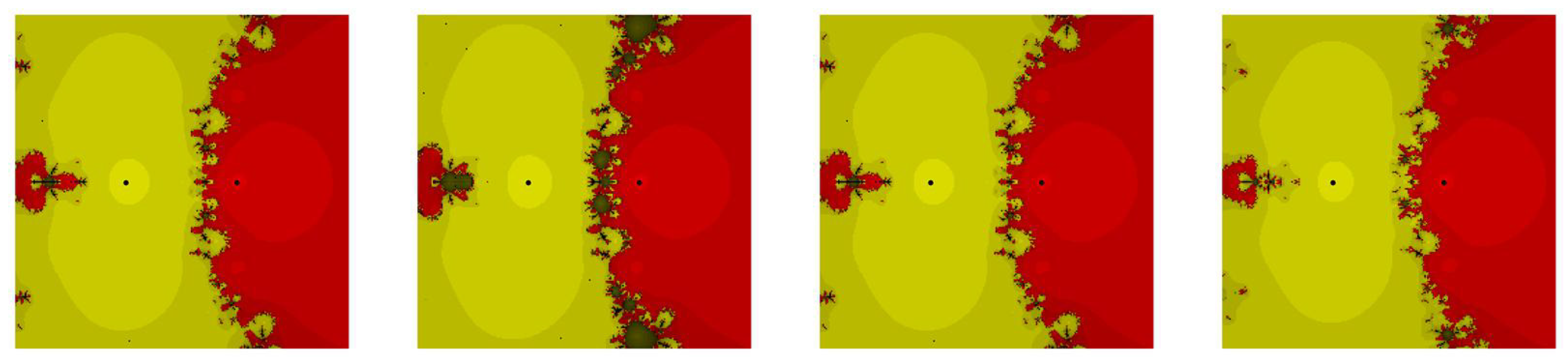
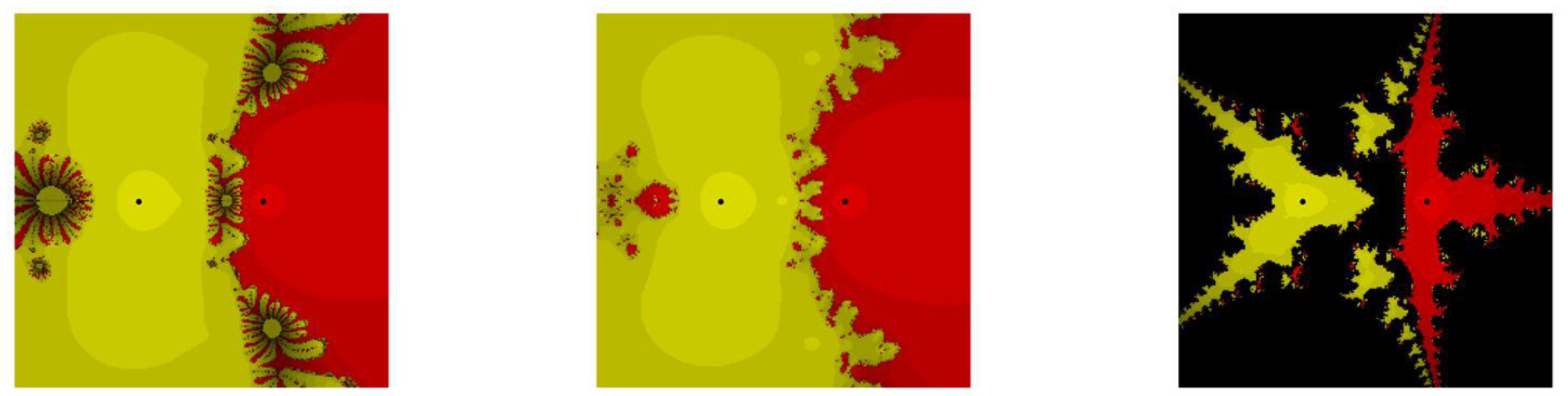
5. Graphical Comparison by Means of Attraction Basins

It is known that a good selection of initial guesses plays a definitive role in iterative methods—in other words, that all methods converge if the initial estimation is chosen suitably. We numerically approximate the domain of attraction of the zeros as a qualitative measure of how demanding the method on the initial approximation of the root is. In order to graphically compare by means of attraction basins, we investigate the dynamics of the new methods $PM{1}_8$, $PM{2}_8$, $PM{3}_8$ and $PM{4}_8$ and compare them with available methods from the literature, namely $S{M}_8$, $K{T}_8$ and $K{M}_8$. For more details and many other examples of the study of the dynamic behavior for iterative methods, one can consult [26,27,28,29].

Let $Q:\mathbb{C}\to \mathbb{C}$ be a rational map on the complex plane. For $z\in \mathbb{C}$, we define its orbit as the set $orb\left(z\right)=\{z,Q\left(z\right),Q^2\left(z\right),\cdots \}$. A point $z_0\in \mathbb{C}$ is called a periodic point with minimal period m if $Q^m\left(z_0\right)=z_0$, where m is the smallest positive integer with this property (and thus $\{z_0,Q\left(z_0\right),\cdots ,Q^{m-1}\left(z_0\right)\}$ is a cycle). The point having minimal period 1 is known as a fixed point. In addition, the point $z_0$ is called repelling if $|Q^{\prime }\left(z_0\right)|>1$, attracting if $|Q^{\prime }\left(z_0\right)|<1$, and neutral otherwise. The Julia set of a nonlinear map $Q\left(z\right)$, denoted by $J\left(Q\right)$, is the closure of the set of its repelling periodic points. The complement of $J\left(Q\right)$ is the Fatou set $F\left(Q\right)$.

In our case, the methods $PM{1}_8$, $PM{2}_8$, $PM{3}_8$ and $PM{4}_8$ and $S{M}_8$, $K{T}_8$ and $K{M}_8$ provide the iterative rational maps $Q\left(z\right)$ when they are applied to find the roots of complex polynomials $p\left(z\right)$. In particular, we are interested in the basins of attraction of the roots of the polynomials where the basin of attraction of a root $z^{*}$ is the complex set $\{z_0\in \mathbb{C}:orb\left(z_0\right)\to z^{*}\}$. It is well known that the basins of attraction of the different roots lie in the Fatou set $F\left(Q\right)$. The Julia set $J\left(Q\right)$ is, in general, a fractal and, in it, the rational map Q is unstable.

For a graphical point of view, we take a $512\times 512$ grid of the square $[-3,3]\times [-3,3]\subset \mathbb{C}$ and assign a color to each point $z_0\in D$ according to the simple root to which the corresponding orbit of the iterative method starting from $z_0$ converges, and we mark the point as black if the orbit does not converge to a root in the sense that, after at most 15 iterations, it has a distance to any of the roots that is larger than ${10}^{-3}$. We have used only 15 iterations because we are using eighth-order methods. Therefore, if the method converges, it is usually very fast. In this way, we distinguish the attraction basins by their color.

Different colors are used for different roots. In the basins of attraction, the number of iterations needed to achieve the root is shown by the brightness. Brighter color means less iteration steps. Note that black color denotes lack of convergence to any of the roots. This happens, in particular, when the method converges to a fixed point that is not a root or if it ends in a periodic cycle or at infinity. Actually and although we have not done it in this paper, infinity can be considered an ordinary point if we consider the Riemann sphere instead of the complex plane. In this case, we can assign a new “ordinary color” for the basin of attraction of infinity. Details for this idea can be found in [30].

We have tested several different examples, and the results on the performance of the tested methods were similar. Therefore, we merely report the general observation here for two test problems in the following

Table 6. Test problems $p_1$ and $p_2$ and their roots.

Test Problem	Roots
$p_1\left(z\right)=z^2-1$	$1,-1$
$p_2\left(z\right)=z^2-z-1/z$	$1.46557,-0.232786\pm 0.792552i$

.

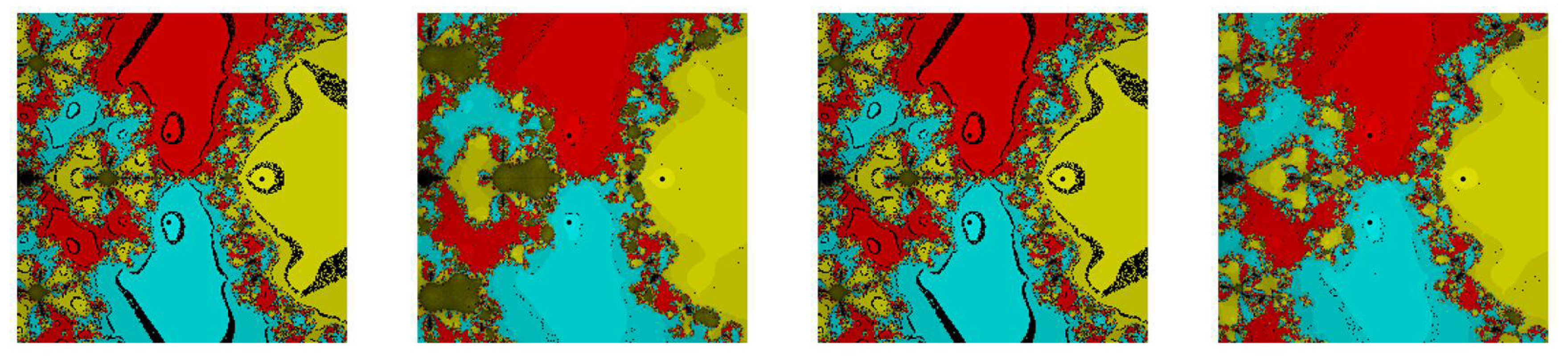
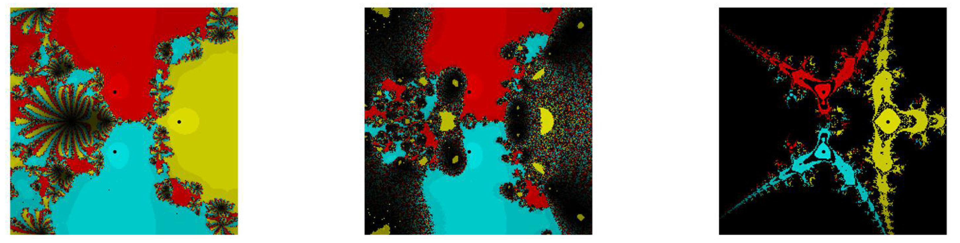
From Figure 1 and Figure 2, we conclude that our methods, namely, $PM{1}_8,PM{3}_8$ and $PM{4}_8$, are showing less chaotic behavior and have less non-convergent points as compared to the existing methods, namely $S{M}_8$ and $K{M}_8$. In addition, our methods, namely, $PM{1}_8,PM{3}_8$ and $PM{4}_8$, have almost similar basins of attraction to $K{T}_8$. On the other hand, Figure 3 and Figure 4 confirm that our methods, namely, $PM{1}_8,PM{2}_{8}PM{3}_8$ and $PM{4}_8$, have less divergent points as compared to the existing methods, namely $K{T}_8$ and $K{M}_8$. There is no doubt that the $S{M}_8$ behavior is better than all other mentioned methods, namely, $PM{1}_8,PM{3}_8$ and $PM{4}_8$ in problem $p_2\left(z\right)$ in terms of chaos.

6. Conclusions

In this study, we present a new technique of eighth-order in a general way. The main advantages of our technique are that is a derivative free scheme, there is a choice of flexibility at the second substep, and it is capable of generating new 8-order derivative free schemes from every optimal 4-order method employing Steffensen’s or Steffensen-type methods. Every member of (9) is an optimal method according to Kung–Traub conjecture. It is clear from the obtained results in Table 1, Table 2, Table 3, Table 4 and Table 5 that our methods have minimum residual error $\left|f\right(x_j\left)\right|$, the difference between two consecutive iterations $|x_{j+1}-x_j|$, and stable computational convergence order as compared to existing methods, namely, $S{M}_8$, $K{T}_8$ and $K{M}_8$. The dynamic study of our methods also confirms that they perform better than existing ones of similar order.

It is important to note that we are not claiming that our methods will always be superior to these methods. One may obtain different results when they rest them on distinct nonlinear functions because the computational results depend on several constraints, including initial approximation, body structure of the iterative method, the considered test problem, configuration of the used system and programming softwares, etc. In future work, we will try to obtain a new family of high-order optimal derivative free iteration functions that depend on the rational functional approach.