A Continuous Coordinate System for the Plane by Triangular Symmetry

Abstract

The concept of the grid is broadly used in digital geometry and other fields of computer science. It consists of discrete points with integer coordinates. Coordinate systems are essential for making grids easy to use. Up to now, for the triangular grid, only discrete coordinate systems have been investigated. These have limited capabilities for some image-processing applications, including transformations like rotations or interpolation. In this paper, we introduce the continuous triangular coordinate system as an extension of the discrete triangular and hexagonal coordinate systems. The new system addresses each point of the plane with a coordinate triplet. Conversion between the Cartesian coordinate system and the new system is described. The sum of three coordinate values lies in the closed interval [−1, 1], which gives many other vital properties of this coordinate system.

1. Introduction

The concept of the grid is essential and heavily used in digital geometry and in digital image processing. A grid is comprised of discrete points addressed with integer vectors. There are three regular tessellations of the plane, which define the square, hexagonal, and triangular grids (named after the form of the pixels used as tiles) [1]. Most of the applications use the square grid because its orthogonal coordinate system, known as the Cartesian coordinate system (CCS), which fits very well to it. This addresses each square pixel of the grid by a pair of independent integers. The dual of the square grid (the grid formed by the nodes, which are the crossing points of the gridlines) is again a square grid. Therefore, essentially, the same CCS is used as well. Working with real images, we may need to perform operations that do not map the grid to itself, e.g., zooming or rotations. The Cartesian coordinate system allows real numbers to be used in such cases. Moreover, the digitization operation can easily be defined by a rounding operation.

The hexagonal grid, tiling the plane by the same size regular hexagons (hexagonal pixels), has been used for decades in image processing applications [2], in cartography [3,4], in biological simulations [5], and in other fields, since the digital geometry of the hexagonal grid provides better results than the square grid in various cases. In addition, it is used in various table and computer games based on its compactness. It is the simplest 2D grid, since the only usual neighborhood using the nearest neighbors is simpler and less confusing than the two types of neighbors in the square grid [6]. The neighborhood of a pixel contains six other hexagons (see Figure 1a). In contrast to the square grid, the dual of the hexagonal grid is not the hexagonal, but the triangular grid (see Figure 1a,b). Adequate and elegant coordinate systems for these kinds of grids are required for their use in both theory and applications, e.g., in image processing or engineering applications. In Reference [7], a three-coordinate-valued system of zero-sum triplets is used to describe the hexagonal grid capturing the triangular symmetry of the grid. In Figure 1a, the first coordinate value is ascending right-upwardly, the second values are ascending into the right-downward direction, and the third one is ascending into the left-upward direction [7,8]. We should mention that this system could be seen as the extension of the oblique coordinate system using two independent integer values [9] by concerning the third value to obtain zero-sum for every triplet. The digital distance based on the neighborhood relation is computed in Reference [9]. Since the vectors describing the grid are not orthogonal, some geometric descriptions based on Cartesian coordinates are not very clear. However, to simplify the expressions of the constrained three-dimensional coordinate system is recommended. We should also mention that 0-sum triplets allowing real numbers were used in Reference [8] to describe rotations (that may not map the hexagonal grid to itself). In this way, a useful digitization operator is found. Her’s system was mentioned and used in References [10,11] for various imaging-related disciplines.

The triangular grid is the third regular grid. It is generated by tiling the plane regularly with equilateral triangles. Although it is the most complex among the three regular tessellations (it has the largest number and types of neighbors), it has various advantages in applications, e.g., by the flexibility of the used neighborhood. The triangular grid is built by triangles in two different orientations. Moreover, it is not a point lattice since some of the grid vectors, i.e., the vectors connecting the midpoints of triangles with different orientations, do not translate the grid into itself [12]. However, the triangular grid gives a valid alternative for applications in image processing. In some cases, it gives better results than the usual square grid due to its better symmetric properties and larger, natural neighborhood structure. Each pixel has 12 neighbors sharing at least a corner. They are categorized into three types of neighbor relations [13,14]. The triangular grid has similar symmetry to the hexagonal grid. Therefore, in Reference [15], a coordinate system with zero-sum and one-sum triplets are used to describe this grid (the three values are not independent, since this is also a 2D grid, see Figure 1c,d). The angle between any two of the three coordinate axes is 120° as for the hexagonal grid. In this description, two pixels are neighbors if their coordinate values differ by at most one. Moreover, at the closest neighbors, only one coordinate differs [15,16]. Observe that exactly the same coordinate triplets are used on the left and on the right-hand side in Figure 1c,d, respectively, which shows the duality of the triangular and hexagonal grids. In Reference [17], a combinatorial coordinate system was shown that addresses the pixels, the corners, and the edges between them. That coordinate system gives an efficient tool to work with digital cell complexes on the triangular grid. Various image processing algorithms have been defined and implemented for the triangular grid recently such as discrete tomography [18,19], thinning [20], and mathematical morphology [21]. We should also mention that triangulation is a frequently used technique in imaging and computer graphics. However, the obtained grid is usually not the regular triangular grid. Lastly, we should note that several non-regular grids have various applications in 2D and in higher dimensions.

The coordination is vital because it is a leading tool in making a simple, easily usable, and effectively programmable system with integer numbers (coordinates). The isometric transformations are described in Reference [12]. However, up to now, there was no such extension of this coordinate system that is able to address the entire plane. For various applications, including, e.g., arbitrary angled rotations, an extension of the coordinate system is needed. We note here that Her’s zero-sum triplets could match only up to half of the grid points in the triangular grid (Figure 1c,d), and, therefore, the coordinate system addressing the whole plain cannot be used for the triangular grid.

In this paper, we introduce a continuous coordinate system for the plain based on the symmetry of the triangular grid, where every point of the 2D plane has its unique coordinate triplet. We use three coordinate values to describe the triangular grid as in Reference [15] but also to address the points of the plane “between” and “around” the nodes of the dual grid. Our new coordinate system is shown to be an extension of the hexagonal and of the triangular coordinate systems. Moreover, our system builds upon the coordinate system for the so-called, tri-hexagonal grid, also called the three-plane triangular grid in Reference [16].

For further applications, we also provide a mapping between our continuous coordinate system for the triangular grid and the Cartesian coordinate system of the 2D plane.

The rest of this paper is as follows. The next, preliminary section, describes some important discrete coordinate systems and the barycentric coordinate system. The continuous coordinate system for the triangular grid is then introduced in Section 3. Conversions to and from Cartesian coordinates are also presented. Some important properties of the new coordinate system are presented in Section 4. Lastly, conclusions close the paper.

2. Preliminaries

In this paper, as usual, Z³ denotes the cubic grid, whose points are addressed by integer triplets, according to the three coordinates x, y, z.

In order to create a continuous coordinate system for the triangular grid that enables us to uniquely address any point of the triangular grid, we combine discrete triangular coordinate systems from Reference [22] (see also Figure 1 for some examples) with the barycentric coordinate system (BCS), discovered by Möbius (see References [1,23]).

In Figure 2, a coordinate system for the tri-hexagonal grid (the three-plane triangular grid of regions [16]) and its dual is given. This grid resembles a mix of the triangular and hexagonal grids since it is a combination of the one-plane and two-plane grids [7,22]. The new coordinate system will be an extension of the discrete triangular and hexagonal coordinate systems.

Next, a brief description is given for the discrete triangular coordinate system and BCS.

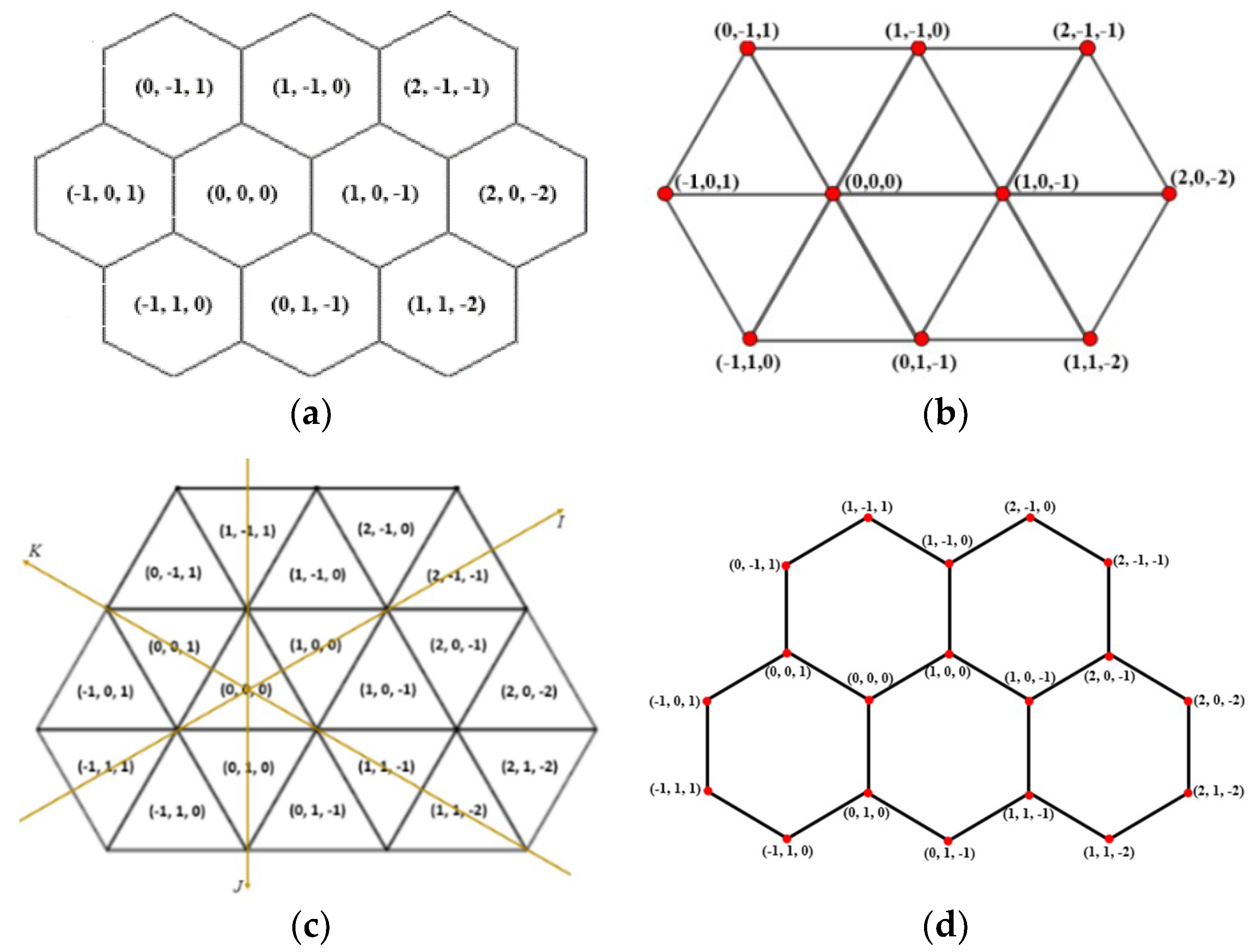
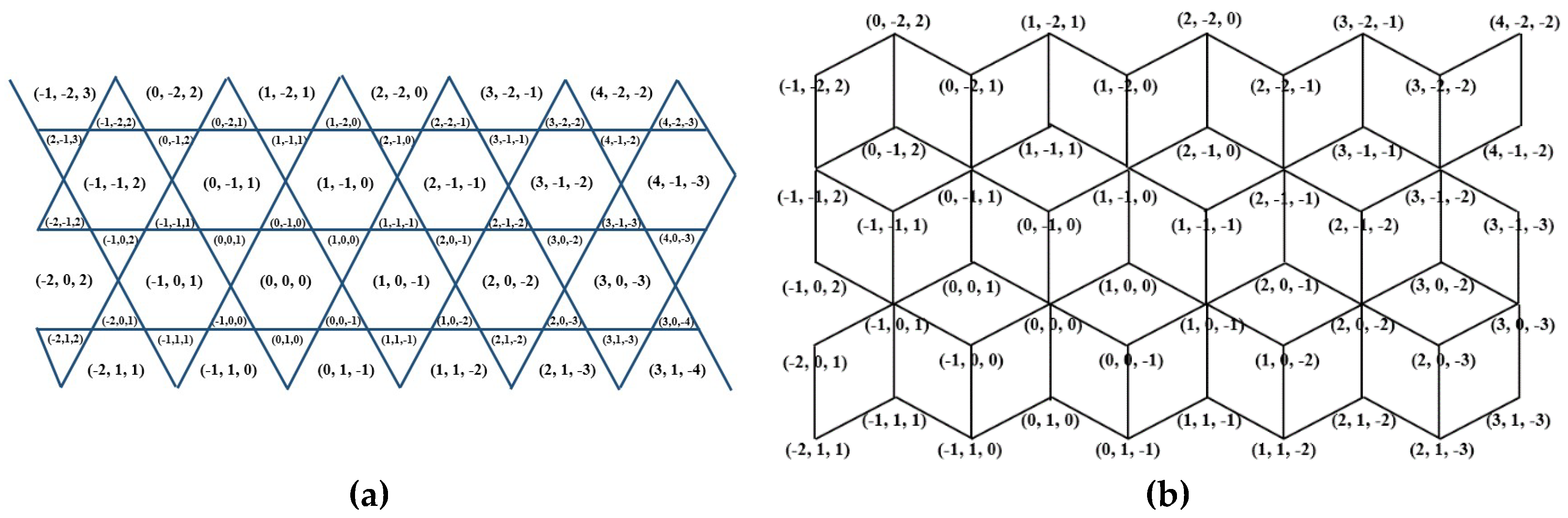
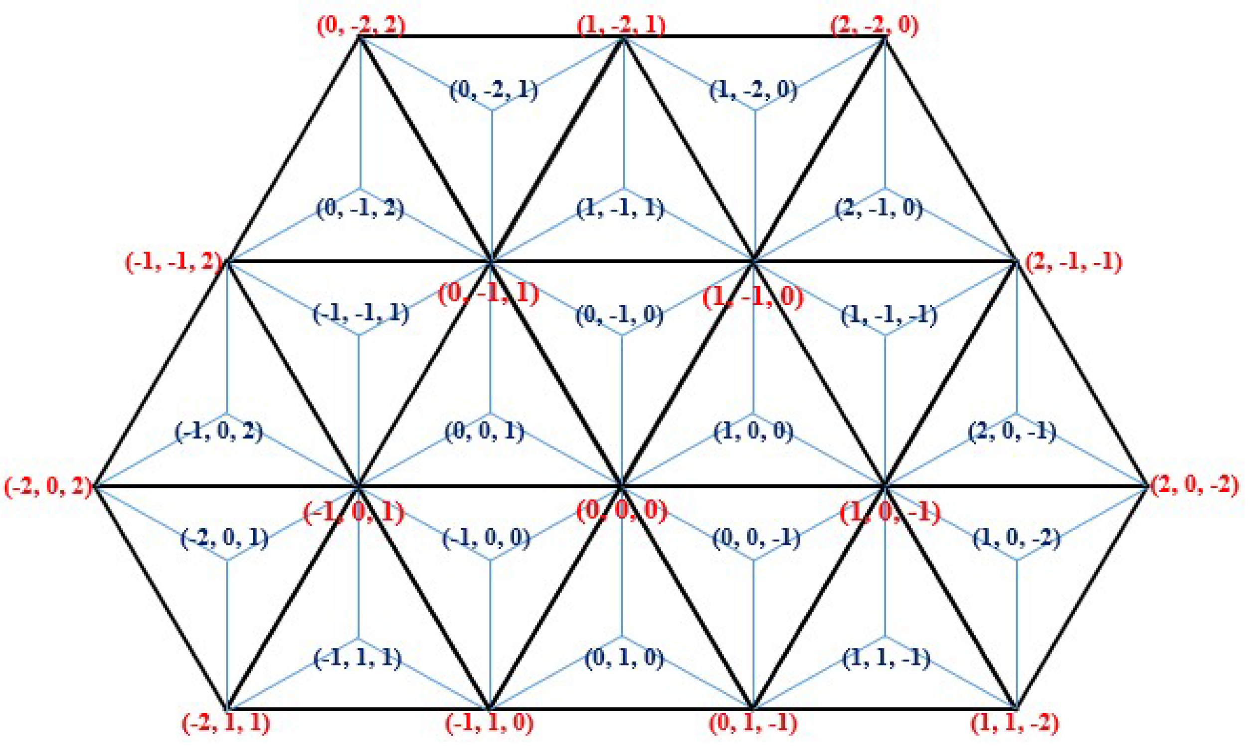
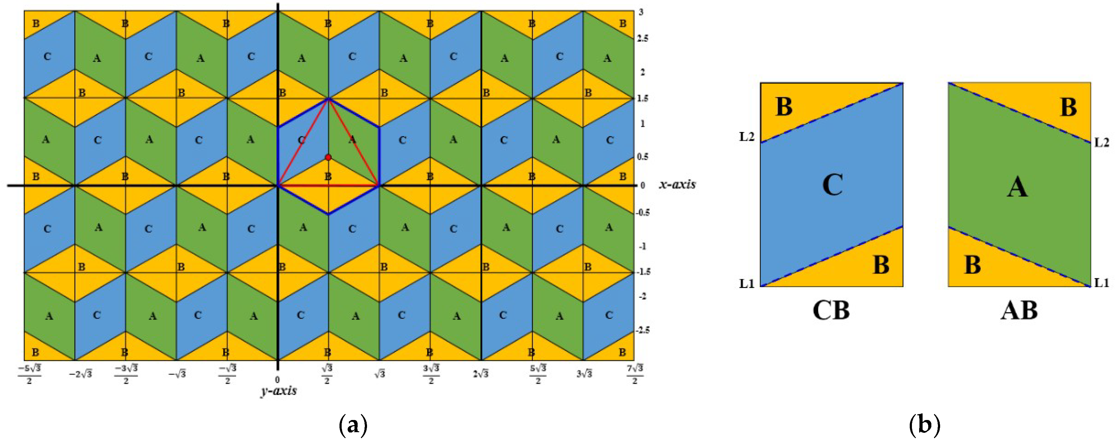
2.1. Discrete Triangular Coordinate System

The discrete Hexagonal Coordinate System uses 0-sum triplets (Figure 1a,b). The discrete Triangular Coordinate System [22] is a symmetric coordinate system that addresses each pixel by an integer triplet. The three coordinate axes have angles of 120° as in the hexagonal grid. The sum of the triplets is equal to 0 or 1, which refers to the two types of orientations of triangles (△, ▽). The triangles with zero-sum are the “even” triangles (△), and the triangles with one-sum triplets are the “odd” triangles (▽) (see Figure 1).

For finding an appropriate extension to this system that is able to address all points of the 2D plane, we start by addressing the midpoints of triangles with integer triplets of +1 and −1 sum. Therefore, we call them “positive △” and “negative ▽” triangles, respectively. According to Figure 3, the coordinate system of Figure 2b is used to address midpoints of triangles of the triangular grid. Observe that each triplet assigned to a midpoint (see the blue triplets in Figure 3) builds up from the coordinate values shared by two of the corners of the given pixel (see the three red triplets around each blue triplet). There is already an important difference between our proposed and Her’s zero-sum coordinate system, which includes the use of zero-sum triplets to address these midpoints as well (actually, three fractional values for each midpoint), which was a very good and efficient choice to extend the coordinate system of the hexagonal grid. However, it does not meet our requirements. Therefore, we have fixed these coordinate values in another way. We should also mention that Her’s system inside the regular triangles can be seen as an application of the barycentric coordinate system (see next subsection) based on the values assigned to the corners of the triangle.

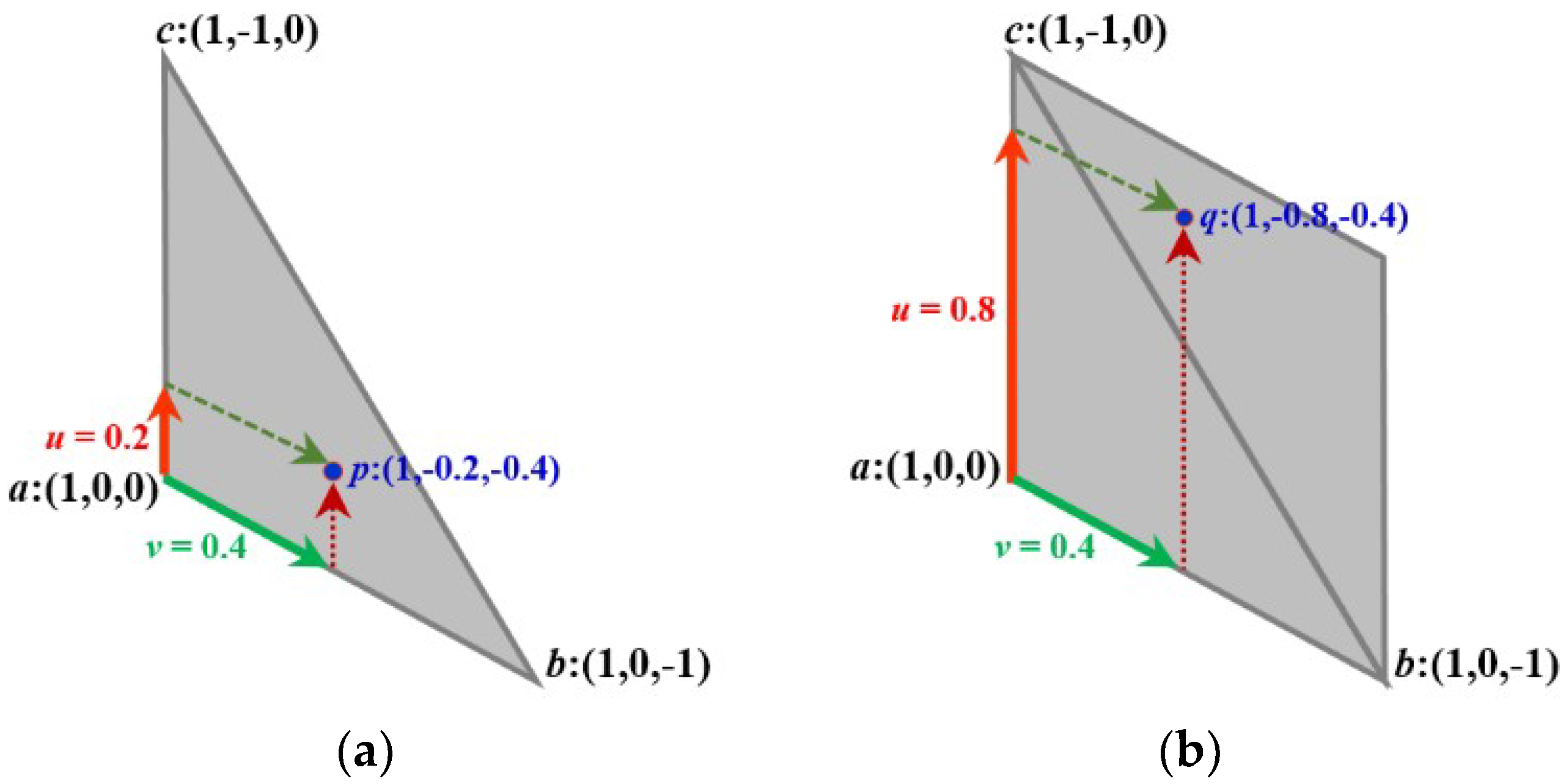
2.2. The Barycentric Coordinate System (BCS)

One of the main motivations of the barycentric technique is to use a coordinate system only for a finite (bordered) segment of the plane, which is also more “balanced” inside this region than the values of the Cartesian frame.

The barycentric technique uses coordinate triplets to address any points inside (and on the border) of a given triangle. We put three one-sum weights, (w, v, u), to the corners known as a, b, and c of the triangle and the mass center p inside the triangle is assigned to the triplet of weights. It is also known that, if the area of the triangle abc is one unit, then the areas of bcp, acp, and abp are exactly w, v, and u, respectively. The coordinates of p can be computed from the coordinates of the corners of the triangle by weighted average, i.e., p = wa + vb + uc (where p, a, b, and c are the vectors representing the positions of these points).

This formula can easily be transformed to the following formula using the fact that w = 1 − v − u:

p = a + v (b − a) + u (c − a)

(1)

Actually, since the three barycentric coordinate values (w, v, and u) of point p are not independent (sum of 1), we may use only two of them, v and u, to address point p similarly as in an oblique coordinate system. One may understand Equation (1) as stating that the starting point is a, and we can go to the direction of b and the direction of c by some distance, which is indicated by v and u, respectively. However, in our approach, the starting point a is the midpoint of the regular triangle and, according to the values of v and u, the coordinate triplet for point p is calculated (see Figure 4 and Example 1).

In the classical barycentric technique, the point is considered to be inside a triangle, as long as the sum of (u and v) is between 0 and 1: 0 < u + v < 1. If the sum is equal to 1, then the point will be on the edge (cb), while it will be out of the triangle if the sum is less than 0 or greater than 1 (see Figure 4a). Now, we relax the condition of the barycentric technique and allow the sum of u and v to be any real number between 0 and 2 besides the conditions 0 ≤ u ≤ 1 and 0 ≤ v ≤ 1 hold (see Figure 4b). In this way, we may also address some points outside of the triangle. In Figure 4 and Example 1, a composition of the barycentric technique and the discrete coordinate system (assigned to the corners of an isosceles triangle in the regular triangle) is given to address other points of the plane.

Example 1.

Consider the triangle defined by corners (1, 0, 0), (1, 0, −1), and (1, −1, 0), which represent the three vertices a, b, and c, respectively. Let u = 0.2 and v = 0.4, where 0 < u + v < 1. Then, based on Equation (1), the coordinate triplet of point p is (1, −0.2, −0.4). If u = 0.8 and v = 0.4 (0 < u + v < 2), then the coordinate triplet of point q is (1, −0.8, −0.4) (see Figure 4).

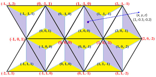
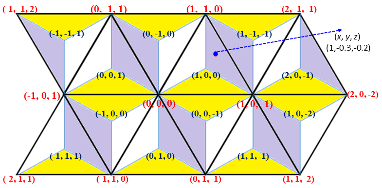
3. Continuous Coordinate System for Reflecting the Triangular Symmetry

In order to create a continuous triangular coordinate system that works efficiently, we combine the discrete coordinate system for the triangle grid with BCS. In the discrete triangular coordinate system, integer coordinate triplets with various sums were used. In BCS, coordinate triplets with fractional values address the points inside a triangle. We develop a new system, which uses triplets on the entire plane. We start by dividing each equilateral triangle of the triangular grid into three isosceles obtuse-angled triangles, which will possess areas A, B, and C, as shown in Figure 5. In this case, the midpoint m between areas will be the start point (the red point), which is represented by the letter a in Equation (1). This point will be used to calculate the coordinates of the points in the three areas A, B, and C.

As we have already mentioned above, we use coordinate triplets with sum +1 and −1 for these midpoints, depending on the orientation of the original triangle. The sum of 1 represents the midpoint of the positive triangles △ and the sum of −1 represents the midpoint of negative triangles ▽. Therefore, using the barycentric Equation (1) based on these midpoints, we obtain a unique triplet for each point in each area of the plane, which we will describe below.

Based on the barycentric Equation (1), we know that the values u and v are limited by 0 ≤ u + v ≤ 1 (inside or on the border of the given triangle), which gives the ability to address the points inside areas A, B, and C of each type of triangle (△, ▽), separately. However, let us consider the case in which the sum of u and v satisfies 0 ≤ u + v ≤ 2, such that the conditions 0 ≤ u ≤ 1 and 0 ≤ v ≤ 1 hold. Then, consequently, each midpoint can be used to address not only the points in the area located in this original triangle but also the points in the neighboring area denoted with the same letters. To illustrate this, the green area in Figure 6a can be completely addressed by using either midpoint a⁽⁺⁾ or a⁽⁻⁾ as the starting point in Equation (1).

Proposition 1.

To address the points inside a rhombus A, B, or C, the coordinate triplet of a point does not depend on the choice of whether the midpoint of the positive or the negative triangle is used for addressing.

Proof. 

Assume point (p) in area A of the negative triangle. Let a⁽⁺⁾ = (a₁, a₂, a₃), a⁽⁻⁾ = (a₁, a₂ − 1, a₃ − 1), p = (p₁, p₂, p₃), b = (b₁, b₂, b₃), and c = (c₁, c₂, c₃) where a⁽⁺⁾ is the midpoint of the positive triangle and a⁽⁻⁾ is the midpoint of the negative one (see Figure 7).

As we mentioned earlier, each triplet assigned to a midpoint builds up from the coordinate values shared by two of the corners of the given pixel (see Section 2.1). Thus, we have some equalities.

In the positive triangle, we have:

a₁ = b₁ = c₁, b₂ = a₂, c₃ = a₃ and c₂ = a₂ − 1,

In the negative triangle, we have:

a₁ = b₁ = c₁, b₂ = a₂, c₃ = a₃ and b₂ = a₂ − 1.

Now, to compute the first coordinate value, a₁, from the positive triangle, we have the following.

p₁₍₊₎= a₁ + v (b₁ − a₁) + u (c₁ − a₁) since a₁ = b₁ = c₁ then p₁₍₊₎ = a₁.

From the negative side, we have the following.

p₁₍₋₎ = a₁ + (1 − v) (b₁ − a₁) + (1 – u) (c₁ − a₁) then also p₁₍₋₎ = a₁.

For the second coordinate value, a₂, from the positive triangle, we have the following.

p₂₍₊₎ = a₂ + v (b₂ − a₂) + u (c₂ − a₂),

since b₂ = a₂, then:

p₂₍₊₎ = a₂ + u (c₂ − a₂).

Using c₂ = a₂ − 1, we get p₂₍₊₎ = a₂ − u.

From the negative side, we have the following.

p₂₍₋₎ = (a₂ − 1) + (1 − v) (b₂ − (a₂ − 1)) + (1 − u) (c₂ − (a₂ − 1)),

since b₂ = (a₂ − 1), it is:

p₂₍₋₎ = (a₂ − 1) + (1 − u) (c₂ − (a₂ − 1)),

since c₂ = a₂, then we have p₂₍₋₎ = a₂ − u.

Lastly, for the third coordinate value, a₃, from the positive triangle, we have:

p₃₍₊₎ = a₃ + v (b₃ − a₃) + u (c₃ − a₃).

Since c₃ = a₃,

p₃₍₊₎ = a₃ + v (b₃ − a₃).

Furthermore, b₃ = a₃ – 1, which yields to p₃₍₊₎ = a₃ − v.

From the negative side, we have the following.

p₃₍₋₎= (a₃ − 1) + (1 − v) (b₃ − (a₃ − 1)) + (1 − u) (c₃ − (a₃ − 1)).

Since c₃ = a₃ − 1 and b₃ = a₃, it can be written as:

p₃₍₋₎= (a₃ − 1) + (1 − v) (b₃ − (a₃ − 1)) = a₃ − v.

Having the point inside other regions, the proof goes in a similar manner. □

As we have already mentioned, a popular way to understand BCS for a point (inside a triangle) goes by the ratio of the areas defined by the triangles determined by the point and two of the triangle corners. In fact, our system uses a similar technique to address the points inside a triangle since it is stated in the next corollary based on the previous proposition.

Corollary 1.

Let p be any point inside or on the border of an obtuse-angled triangle determined by a midpoint a = (a₁, a₂, a₃), and corners b = (b₁, b₂, b₃), c = (c₁, c₂, c₃). Let the barycentric coordinates of p be (w, v, u), with w + v + u = 1, i.e., by assigning these weights to a and b and c, respectively, the weighted midpoint is at p. Then, the coordinates of p = (p₁, p₂, p₃) are exactly p_i = w a_i + v b_i + u c_i for i = 1, 2, 3.

Notice that the three points a, b, and c above must have a fixed coordinate value (depending on the type of the triangle). The weighted average of this coordinate value will be the same for any point inside or on the border of this obtuse-angled triangle.

As we have seen a given triplet of corners, including a midpoint can be used to address points not only on the inside but also on the border of the triangle determined by them. The type of these regions is important in this issue. In Figure 6b, the thick, dark blue line shows the entire area that the positive midpoint can address. The key issue is to use triplets of the discrete coordinate system and to use only two barycentric fractional values inside, by using the directions of the sides of the appropriate rhombus in which the point is located. The sides of a rhombus are actually parallel to two of the coordinate axes.

Hereafter, for simplicity, we will use only the positive midpoints for further calculations, while ignoring the negative ones. The triangular plane can be seen in Figure 8a.

In the next two subsections, we will illustrate the conversion between the continuous coordinate system to/from the Cartesian coordinate system. Namely, we can convert the coordinate triplet of a certain point in our new coordinate system to its corresponding Cartesian coordinates and vice versa.

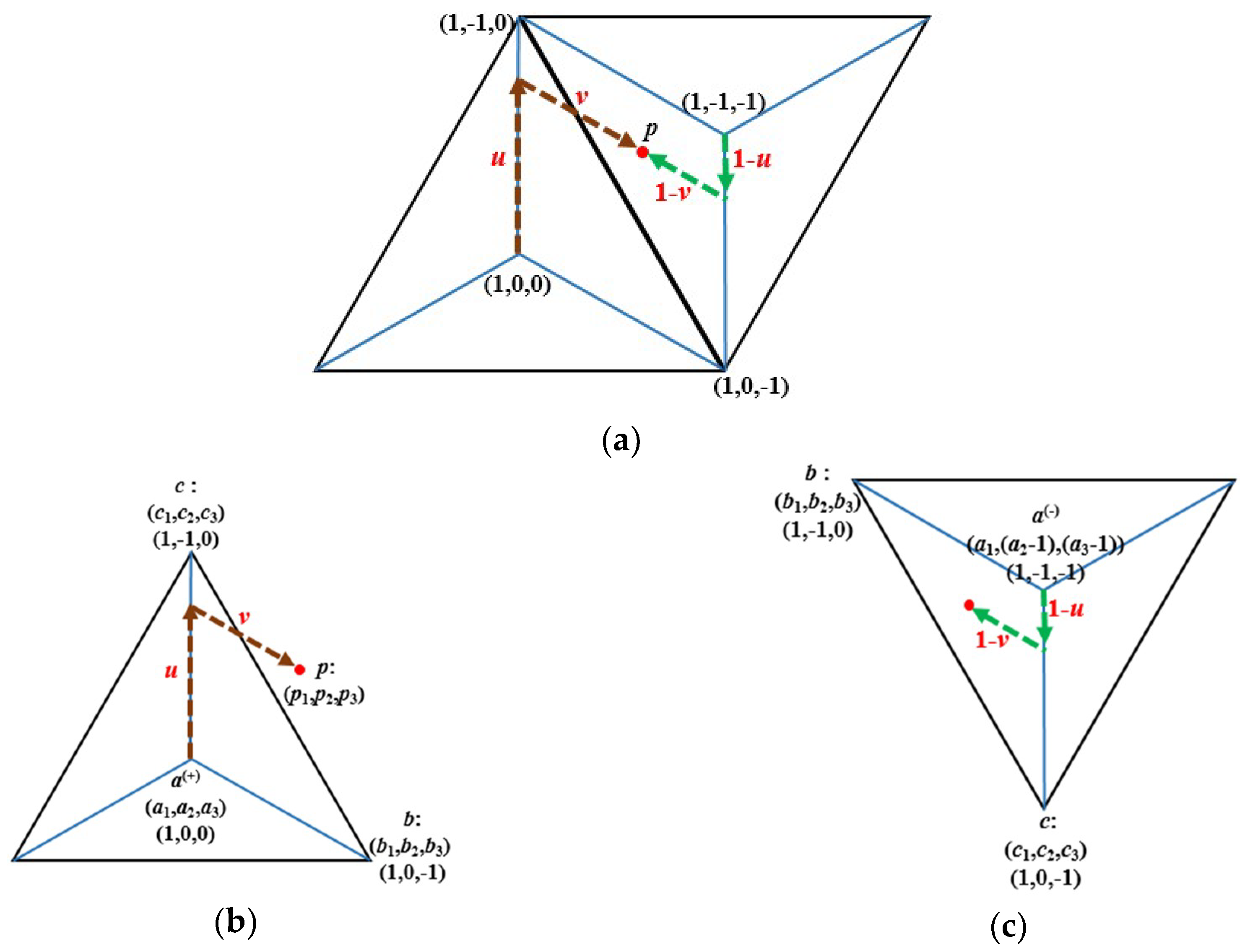
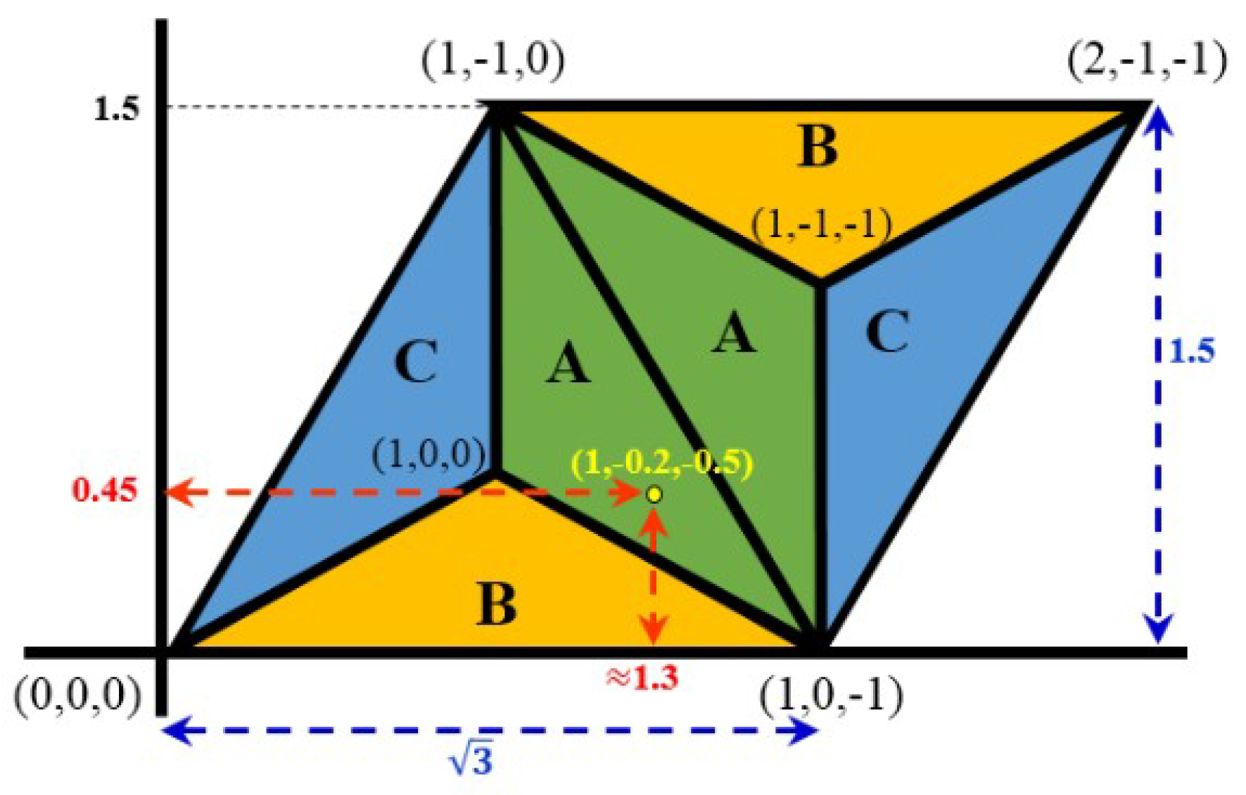
3.1. Converting Triplets to Cartesian Coordinates

Assume that we use (i, j, k) as a coordinate triplet of a point, where I, J, and K are the axes of the triangular plane (see Figure 1), and suppose (x, y) is used to indicate the same point in the Cartesian plane where X and Y are the axes.

For the conversion, we fix the side-length of the triangle of the triangular grid to $\sqrt{3}$. Consequently, its height is 1.5 (see the dashed blue lines in Figure 9). Then, the following matrix equation computes the corresponding coordinate values x and y for the given triplet (i, j, k):

$$\left(\begin{array}{ccc}\frac{\sqrt{3}}{2}& 0& -\frac{\sqrt{3}}{2}\\ \frac{1}{2}& -1& \frac{1}{2}\end{array}\right)·\left(\begin{array}{c}i\\ j\\ k\end{array}\right)=\frac{1}{2}·\left(\begin{array}{c}\sqrt{3}\left(i-k\right)\\ i-2j+k\end{array}\right)=\left(\begin{array}{c}x\\ y\end{array}\right)$$

(2)

Example 2.

Let (1, −0.2, −0.5) be a point in the triangular plane. Then, based on (2):

$$\left(\begin{array}{ccc}\frac{\sqrt{3}}{2}& 0& -\frac{\sqrt{3}}{2}\\ \frac{1}{2}& -1& \frac{1}{2}\end{array}\right)·\left(\begin{array}{c}1\\ -0.2\\ -0.5\end{array}\right)\approx \left(\begin{array}{c}1.3\\ 0.45\end{array}\right)$$

Thus, (x, y) ≈ (1.3, 0.45), as shown in Figure 9.

3.2. Converting Cartesian Coordinates to Equivalent Triplets

One of the simplest ways to do such a conversion is to determine the midpoint and the two corner points, which defines the triangle in which the given point locates (inside or on the border). Then, by computing the barycentric coordinates (weights) of the point with respect to these triangle corners, by Corollary 1, the continuous coordinate triplet is computed. In this subsection, we present a slightly different method with little more details to convert Cartesian coordinates to continuous triangular coordinates.

As we already mentioned earlier, the midpoints of positive triangles are used to address all points in the triangular plane. Therefore, every positive midpoint will address areas A, B, and C in neighbor (negative) triangles, as already seen in Figure 6b. Consequently, the triangular plane will be re-structured, which can be seen in Figure 8a. However, two kinds of rectangles can be clearly distinguished in this plane, called CB and AB (see Figure 8b).

We may start by specifying the area (i.e., rhombus) A, B, or C that a Cartesian point (x, y) belongs to. Then, we can use appropriate formulae that are assigned to each type of area, which is a process we will describe later in this section (see

Table 1. The coordinate triplets formulae, based on area type, where $\langle \dots \rangle$ is a rounding operation *.

Coordinate Triplet	Area A	Area B	Area C
i	$\langle \frac{x}{\sqrt{3}}\rangle +\langle \frac{y}{3}\rangle$	$\frac{x\sqrt{3}}{3}+y+j$	$\frac{2x}{\sqrt{3}}+k$
j	$\frac{i+k}{2}-y$	$\langle \frac{-2y}{3}\rangle$	$\frac{i+k}{2}-y$
k	$i-\frac{2x}{\sqrt{3}}$	$i-\frac{2x}{\sqrt{3}}$	$\langle \frac{y}{3}\rangle -\langle \frac{x}{\sqrt{3}}\rangle$

* rounding operation returns the nearest integer to the real number, such that numbers exactly the same distance from two integers are rounded to the larger absolute valued one, e.g., $\langle 1.5\rangle =2$, $\langle -1.5\rangle =-2$ and $\langle -0.4\rangle =0$.

). Hence, the following three steps are used to specify the area.

Step 1

Which quarter of the Cartesian plane is involved? Note that the 1st and 3rd quarters have the same structure, while the 2nd and 4th quarters have another one.

Step 2

Which rectangle is involved (AB or CB)?

Step 3

Which area is involved (A, B, or C)?

We show how these steps can be computed by pseudo codes. The first step is the easiest one since we can inquire whether the values of (x, y) are greater or equal to zero or not. Then, this task is completed and the involved quarter is specified (see Code 1).

Code 1.

• IF ((x ≥ 0) AND (y ≥ 0)) OR ((x < 0) AND (y < 0))
• THEN “1st or 3rd quarter”
• ELSE “2nd or 4th quarter”

To complete the second step, note that the basic measurements of every rectangle are known, with a height and width equal to 1.5 and $\left(\sqrt{3}/2\right)$, respectively. Then, the CB rectangle is involved whenever the integer part of x and y, are both even or both odd. Otherwise, the AB rectangle is involved. See Code 2 to clarify this step.

Code 2.

• IF ((int ($2x/\sqrt{3}$) mod 2 = 0) AND (int (y/1.5) mod 2) = 0) OR
• (int ($2x/\sqrt{3}$) mod 2 = 1) AND (int (y/1.5) mod 2) = 1))
• THEN “CB Rectangle is involved”
• ELSE “AB Rectangle is involved”

where:

• int takes the integer part of the (decimal) number,
• mod is the modulus (or remainder, here after division by two).

Now, the involved rectangle is specified and the third step follows. Since we have two types of rectangles AB and CB, and they are symmetric, we will discuss only one of them known as type AB rectangles.

In rectangle AB, a point (x, y) will belong to either part A or part B. To decide which one is involved, we consider Line 1 (L1) and Line 2 (L2) in Figure 8b, where they divide the rectangle into parts A and B. If the point is between L1 and L2, then part A is involved. Otherwise, it is in part B. However, L1 and L2 are considered to be within the area A in cases when the point is on the lines. Equations (3) and (4) of a straight line are used for Line 1 and Line 2, respectively.

m·x + r₁ − y = 0,

(3)

m·x + r₂ − y = 0,

(4)

where:

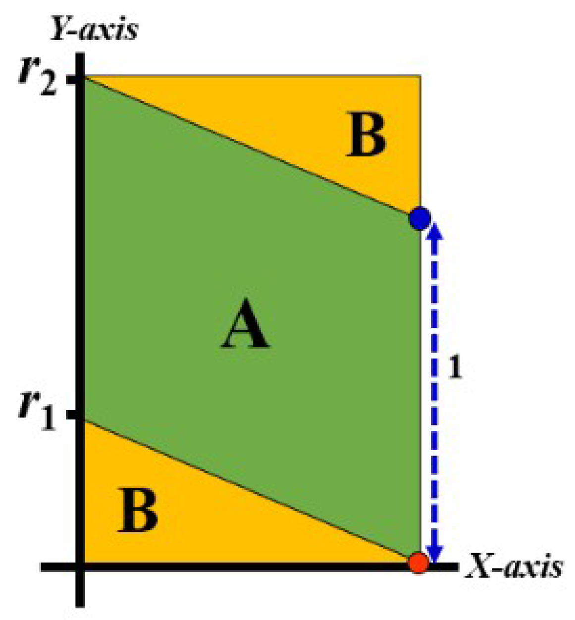
• m is the slope of L1 and L2, which is a constant here, equal to $\left(-\sqrt{3}/3\right)$,
• r₁ and r₂ are the y-axis intercept with L1 and L2, respectively, where r₂ = r₁ + 1

This step is started by substituting the point (x, y) in Equations (3) and (4). Then, it is determined that part A is involved if the left side of Equation (3) is not greater than 0 and the left side of Equation (4) is not less than 0. Otherwise, part B is involved. Code 3 is used to clarify this step.

Code 3.

• IF ((r₁ $- x\sqrt{3}/3$ − y) ≤ 0) AND ((r₂ $- x\sqrt{3}/3$ − y) ≥ 0)
• THEN “Area A is involved”
• ELSE “Area B is involved”

The y-axis intercept with Line 1, r₁, in area AB, is computed by computing any point (x, y) on Line 1. Therefore, the point at the bottom-right corner of rectangle AB is computed for this purpose (see the red point in Figure 10). Hence, Equation (5) is used to find the value of r₁. In Equation (5), we used the modulus (mod) as a function naturally extended to real numbers, i.e., it gives the remainder after the division by a real number (and that is between 0 and the divisor). Moreover, by adding 1 to r₁, we get the value of the y-axis intercept with Line 2, r₂ (see Code 3).

$$r_1=y-\left(y mod \frac{3}{2}\right)+\frac{\sqrt{3}}{3}·\left(x+\frac{\sqrt{3}}{2}- \left(x mod \frac{\sqrt{3}}{2}\right)\right)$$

(5)

Similar strategies are used when the CB rectangle is involved, taking care that the slopes of Line 1 and Line 2 will be equal to $\left(\sqrt{3}/3\right)$.

Lastly, when the involved area A, B, or C is specified, particular formulae are used that are specified in Table 1. Example 3 is used for a further explanation.

Example 3.

Consider a point with Cartesian coordinates: (x, y) = (1.299, 0.45). In order to convert this Cartesian coordinate pair to its corresponding triangular triplet, the three steps below will be followed.

Step 1

The 1st or 3rd quarter is involved.

Step 2

It’s odd and even. Therefore, rectangle AB is involved.

Step 3

Area A is matched.

Thus, formulae of area A (see Table 1) should be applied in this order, so:

(1) 

i =$\langle 0.75\rangle +\langle 0.15\rangle$= 1 + 0 = 1

(2) 

k = 1 −$\frac{2x}{\sqrt{3}}\approx$−0.500.

(3) 

j$\approx$−y + 0.5 · 0.5 = −0.2

The corresponding triplet is (i, j, k)$\approx$(1, −0.2, −0.5), which is approximately the same as in Example 2, as it should be.

To show the conversion of points on other areas (e.g., Area B or Area C), the following examples are given:

Example 4. (Point in Area B)

(a) 

Converting from Continuous Coordinate System to CCS.

Let (i, j, k) = (0.683, 0, −0.183) be a point in the triangular plane. To convert to CCS, Equation (2) is used:

$$\left(\begin{array}{ccc}\frac{\sqrt{3}}{2}& 0& -\frac{\sqrt{3}}{2}\\ \frac{1}{2}& -1& \frac{1}{2}\end{array}\right)·\left(\begin{array}{c}0.683\\ 0\\ -0.183\end{array}\right)\approx \left(\begin{array}{c}0.75\\ 0.25\end{array}\right)$$

(b) Converting from CCS to a Continuous Coordinate System.

Let (x, y) = (0.75, 0.25). The corresponding Continuous Coordinate System triplet can be calculated based on the three steps above as follows.

Step 1

It belongs to the 1st quarter.

Step 2

It belongs to rectangle CB.

Step 3

Area B is matched.

Thus, formulae of area B from Table 1 are applied in the following order:

(1) 

j = $\langle \frac{-2y}{3}\rangle$ = 0

(2) 

i =$\frac{x\sqrt{3}}{3}+y+j$$\approx$0.433 + 0.25 + 0 = 0.683

(3) 

k =$i-\frac{2x}{\sqrt{3}}$$\approx$0.683 − 0.866 = −0.183

The corresponding triplet is (i, j, k) = (0.683, 0, −0.183), which is exactly the original value.

Example 5.(Point in Area C)

(a) 

Converting from the Continuous Coordinate System to CCS.

Let (i, j, k) = (0.346, −0.626, 0) be a point in the triangular plane. To convert to CCS, we use Equation (2) below.

$$\left(\begin{array}{ccc}\frac{\sqrt{3}}{2}& 0& -\frac{\sqrt{3}}{2}\\ \frac{1}{2}& -1& \frac{1}{2}\end{array}\right)·\left(\begin{array}{c}0.346\\ -0.626\\ 0\end{array}\right)\approx \left(\begin{array}{c}0.299\\ 0.799\end{array}\right)$$

(b) Converting from CCS to a Continuous Coordinate System

Let (x, y) = (0.299, 0.799). The corresponding Continuous Coordinate System triplet can be calculated based on the three steps below.

Step 1

It belongs to the first quarter.

Step 2

It belongs to rectangle CB.

Step 3

Area C is matched.

Thus, formulae of area C from Table 1 are applied in the following order.

(1) 

k =$\langle \frac{y}{3}\rangle -\langle \frac{x}{\sqrt{3}}\rangle$= 0 − 0 = 0

(2) 

i =$\frac{2x}{\sqrt{3}}+k$$\approx$0.346 + 0 = 0.346

(3) 

j =$\frac{i+k}{2}-y$$\approx$0.173 − 0.799 = −0.626

The corresponding triplet is (i, j, k) = (0.346, −0.626, 0), which is exactly the original triplet.

Example 6.(A mid-point)

(a) 

Converting from Continuous Coordinate System to CCS.

Let (i, j, k) = (1, 0, 0) be a point in the triangular plane. To convert to CCS, Equation (2) is used below.

$$\left(\begin{array}{ccc}\frac{\sqrt{3}}{2}& 0& -\frac{\sqrt{3}}{2}\\ \frac{1}{2}& -1& \frac{1}{2}\end{array}\right)·\left(\begin{array}{c}1\\ 0\\ 0\end{array}\right)=\left(\begin{array}{c}\frac{\sqrt{3}}{2}\\ \frac{1}{2}\end{array}\right)$$

(b) Converting from CCS to a Continuous Coordinate System.

Let (x, y) = ($\sqrt{3}/2$, 0.5). The corresponding Continuous Coordinate System triplet can be calculated based on the three steps below.

Step 1

It belongs to the first quarter.

Step 2

Based on Code 2, it belongs to rectangle CB (but, since it is a mid-point, then either rectangle AB or CB may be used).

Step 3

Area B is matched.

Thus, formulae of area B from Table 1 are applied in the following order.

(1) 

j =$\langle \frac{-2y}{3}\rangle$= 0

(2) 

i =$\frac{x\sqrt{3}}{3}+y+j$= 0.5 + 0.5 + 0 = 1

(3) 

k =$i-\frac{2x}{\sqrt{3}}$= 1 − 1 = 0

The corresponding triplet is (i, j, k) = (1, 0, 0), which is exactly the original value.

4. Properties of the Continuous Triangular Coordinate System

In this section, we will focus on the most important properties of this continuous coordinate system.

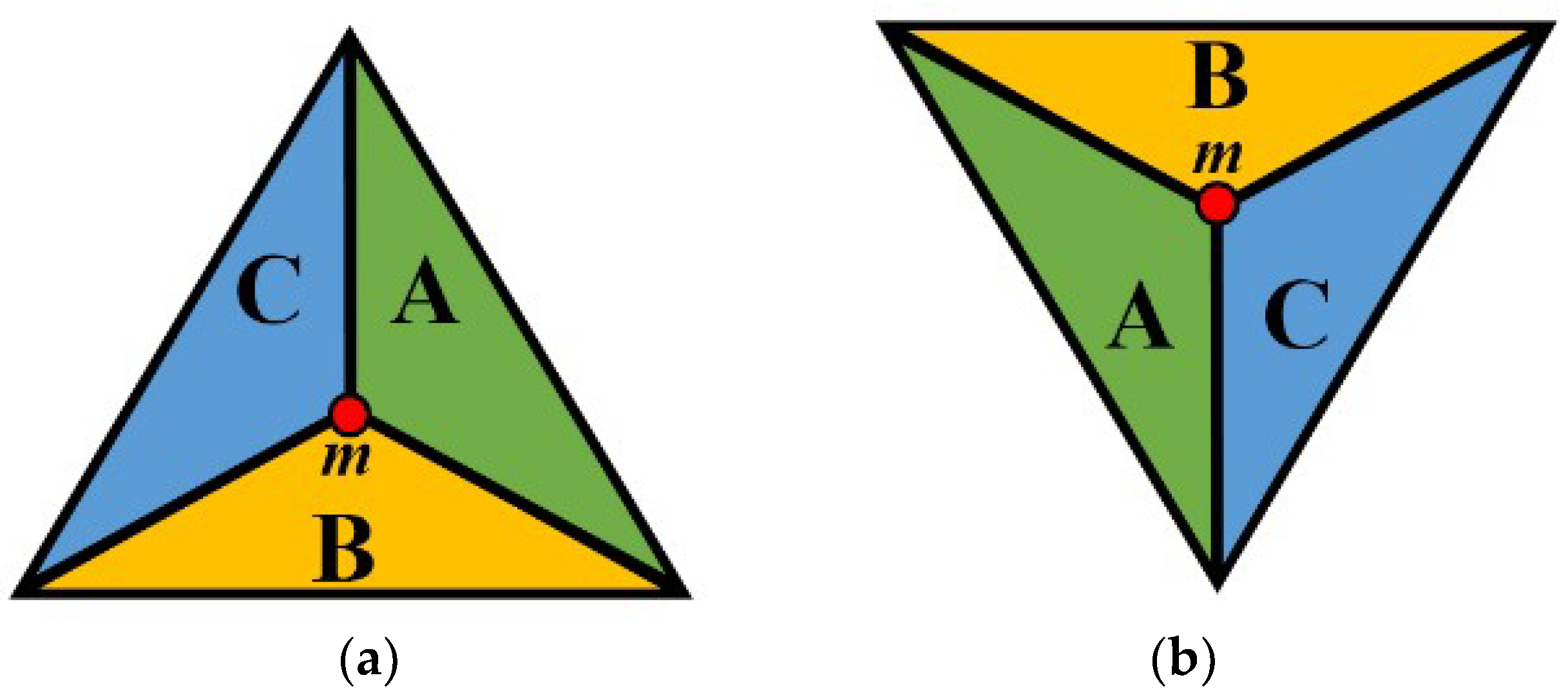
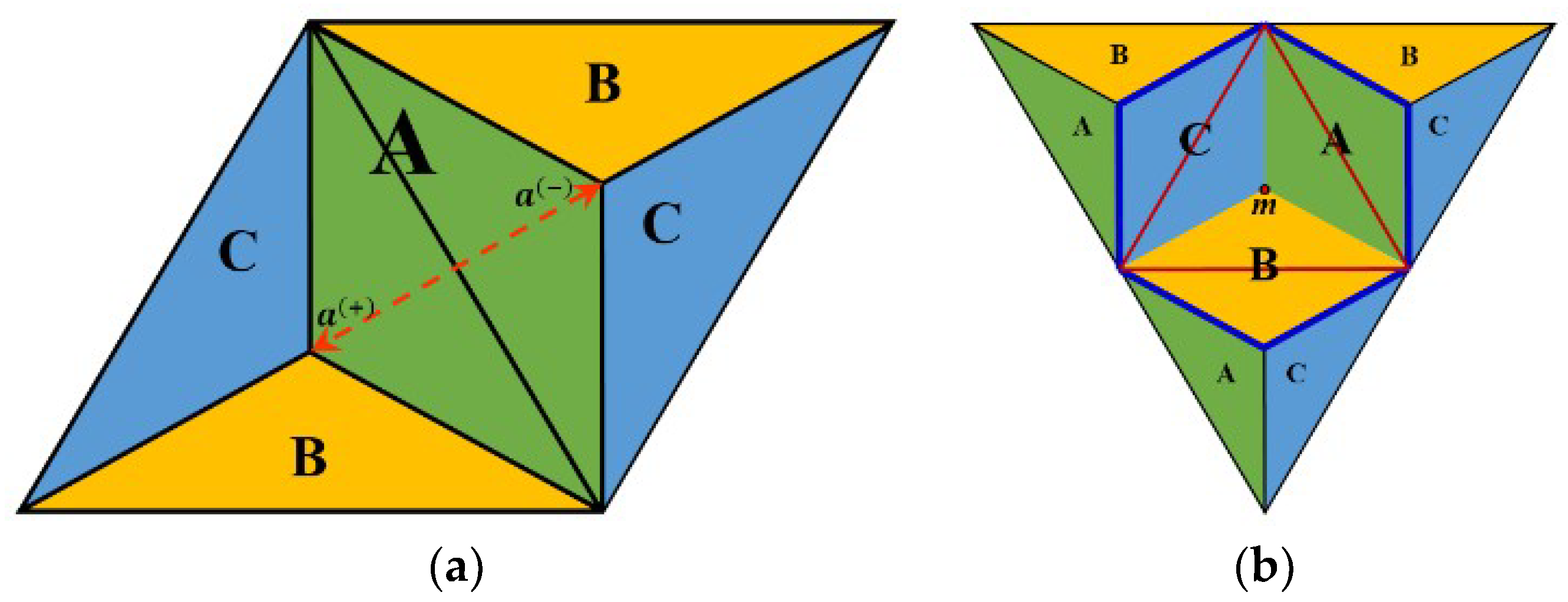
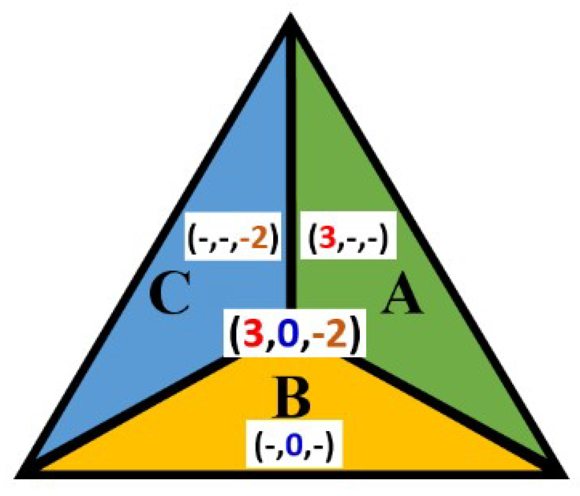
4.1. On the Triplets of a General Point

In Figure 6a, consider the red straight line between a⁽⁺⁾ and a⁽⁻⁾, in the green area. Then, the sum of the coordinate values of the points on this line would change continuously from 1 until −1. Depending on the sum, we can classify the points as follows:

If a point with 3 CV’s sum is:

• equal to 1, then it indicates the positive midpoint (i.e., a⁽⁺⁾);
• equal to −1, then it indicates the negative midpoint (i.e., a⁽⁻⁾);
• equal to 0, then it indicates the point on the triangle’s edge;
• positive, then the point belongs to the positive triangle;
• negative, then the point belongs to the negative triangle.

Theorem 1.

The sum of the coordinate triplet of any point in the plane is in the range of the closed interval [−1, 1].

Proof. 

Consider an area A of a positive triangle with the corners a = (a₁, a₂, a₃), b = (b₁, b₂, b₃), and c = (c₁, c₂, c₃), where b and c are vertices (corners of an equilateral triangle) of the grid, while a is the midpoint of a positive triangle and p = (p₁, p₂, p₃) is a randomly chosen point belonging to this area (inside or on the border of A). Now based on the barycentric Equation (1), we have the following.

$${{\displaystyle \sum }}_{i=1}^3{p}_i={{\displaystyle \sum }}_{i=1}^3{a}_i+v·({{\displaystyle \sum }}_{i=1}^3(c_i-a_i))+u·({{\displaystyle \sum }}_{i=1}^3(b_i-a_i))$$

It is clear that ${{\displaystyle \sum }}_{i=1}^3{a}_i=1$, whereas

$$\begin{array}{ll}\hfill {{\displaystyle \sum }}_{i=1}^3\left(c_i-a_i\right)& =(c_1-a_1)+(c_2-a_2)+(c_3-a_3)\\ & =(c_1+c_2+c_3)-(a_1+a_2+a_3)\\ & =0-1=-1\end{array}$$

Similarly, ${{\displaystyle \sum }}_{i=1}^3\left(b_i-a_i\right)$ = −1.

Then, by substitution, we have the following.

$${{\displaystyle \sum }}_{i=1}^3{p}_i=1-u-v=1-(u+v).$$

(6)

Since 0 ≤ u + v ≤ 2, the maximal and minimal value of the sum of any coordinate triplet is equal to 1 (when u + v = 0) and to −1 (when u + v = 2), respectively. □

Theorem 2.

The sum of the coordinates of a triplet is non-negative in a positive triangle and non-positive in a negative triangle.

Proof. 

Consider a point p that belongs to a positive triangle. Clearly, the coordinates of p are based on u and v such that 0 ≤ u + v ≤ 1. Now, by substituting u + v in Formula (6) (at the proof of Theorem 1, the summation will always be non-negative (moreover, it is positive inside the triangle).

Similarly, let p belong to a negative triangle, then 1 < u + v ≤ 2. Thus, by substituting into Formula (6), the sum will always be a non-positive value. □

Every point in the triangular plane has at least one integer value in its triplet. Moreover, the place of the integer value indicates its area (A, B, or C).

Theorem 3.

The first coordinate value of every point in area A is the same as the first coordinate value of the midpoint. The second coordinate value of every point in area B equals the second coordinate value of the midpoint. Similarly, the third coordinate value of any point in area C equals the third coordinate value of the midpoint (Figure 11).

Proof. 

Consider an area A of a positive triangle with the corners a = (a₁, a₂, a₃), b = (b₁, b₂, b₃), and c = (c₁, c₂, c₃), where b and c are vertices (corners of an equilateral triangle) of the grid, while a is the midpoint and p = (p₁, p₂, p₃) is a randomly chosen point belonging to this area (i.e., inside or on the border of the triangle abc). Since it is area A, we have a₁ = b₁ = c₁. Substituting this into Equation (1), p₁ = a₁ follows for any point p in this area. A similar proof can be considered for areas B and C. □

If a triplet contains two integer values, then the point is located on the line bordering the areas. For example, a triplet of the form (1, 0, k) addresses a point on the line (side of the obtuse-angled triangle) between area A and B (0 ≤ k ≤ −1). However, if three integers are a triplet, then this triplet addresses either a midpoint or a vertex (corner) of a triangle.

4.2. Relation to Discrete Coordinate Systems

In Reference [16], the hexagonal grid is called a one-plane triangular grid since it is a sub-plane of Z³ and because of its symmetry. The triangular grid (nodes of the hexagonal grid) is called a two-plane triangular grid. Combining one-plane and two-plane grids produces the so-called three-plane triangular grid, which is known as the tri-hexagonal grid (Reference [24], Figure 2). In this subsection, their coordinate systems are compared to the new coordinate system.

Theorem 4.

The triplets containing only integers such that their sum equals zero represent exactly the hexagonal grid (one-plane triangular grid).

Proof. 

See Figure 1b for the points of this grid. One may check that exactly those points are addressed with zero-sum integer triplets for which the Cartesian coordinate pair is described below.

$$\mathrm{H}=\left\{\right(x,y\left)\right|x=\left(m\sqrt{3}\right)/2,y=1.5n,\mathrm{where}m,n\mathrm{are}\mathrm{integers}\mathrm{such}\mathrm{that}m+n\mathrm{is}\mathrm{even}\}.$$

 □

Theorem 5.

The triplets containing only integers such that their sum is either 0 or 1 represent exactly the triangular grid (two-plane triangular grid).

Proof. 

See Figure 1d for the points of this grid. The locations of the points with zero-sum coordinate triplets are already known by Theorem 4. Now, we give the locations of the points addressed with 1-sum (integer) triplets.

$$\mathrm{T}=\left\{\right(x,y\left)\right|x=\left(m\sqrt{3}\right)/2,y=1.5n-1,\mathrm{where}m,n\mathrm{are}\mathrm{integers}\mathrm{such}\mathrm{that}m+n\mathrm{is}\mathrm{even}\}.$$

One can easily see that the union of these two sets (H and T) of points gives back exactly the vertices of the hexagons of the figure, i.e., the coordinate system of the dual triangular grid. □

Theorem 6.

The triplets containing only integers such that their sum is either 0 or ±1 represent exactly the tri-hexagonal grid (that is the three-plane triangular grid).

Proof. 

See Figure 3 for the points of this grid. According to Theorem 5, the locations of the zero-sum and one-sum integer coordinate triplets are already shown. We need to show the locations of the points addressed with (integer) triplets that have −1-sum. They are:

$$\mathrm{M}=\left\{\right(x,y\left)\right|x=\left(m\sqrt{3}\right)/2,y=1.5n+1,\mathrm{where}m,n\mathrm{are}\mathrm{integers}\mathrm{such}\mathrm{that}m+n\mathrm{is}\mathrm{even}\}.$$

Actually, the points of this grid, T ∪ H ∪ M, are exactly those that were the base of the method of creating the coordinate system. □

5. Conclusions

The presented continuous coordinate system is an extension of some previously known discrete coordinate systems, e.g., of the symmetric coordinate frame for the triangular grid. This extension is needed and helpful for various applications, where the grid points are not necessarily mapped to grid points, e.g., arbitrary angled rotations, zooming or interpolation of images. We should also mention translations of images [25] since the triangular grid is not a point lattice. Mathematical morphology operators are also based on local translations [21]. Thus, our coordinate system provides a new tool for the research direction as well. The proposed system addresses each point of the 2D (triangular) plane. Conversion to and from the Cartesian coordinate system is provided. These mappings are inverses of each other. Thus, the new coordinate system is ready to use in various applications including those operations that do not necessarily map the grid to itself.

References

1. Coxeter, H.S.M. Introduction to Geometry, 2nd ed.; Wiley: New York, NY, USA, 1969. [Google Scholar]
2. Middleton, L.; Sivaswamy, J. Hexagonal Image Processing—A Practical Approach; Springer: London, UK, 2005. [Google Scholar]
3. Carr, D.B.; Olsen, A.R.; White, D. Hexagon mosaic maps for display of univariate and bivariate geographical data. Cartogr. Geograph. Inform. Syst. 1992, 19, 228–236. [Google Scholar] [CrossRef]
4. Sahr, K. Hexagonal discrete global grid systems for geospatial computing. Arch. Photogramm. Cartogr. Remote Sens. 2011, 22, 363–376. [Google Scholar]
5. Sakai, K.I. Studies on the competition in plants. VII. Effect on competition of a varying number of competing and non-competing individuals. J. Genet. 1957, 55, 227–234. [Google Scholar] [CrossRef]
6. Birch, C.P.; Oom, S.P.; Beecham, J.A. Rectangular and hexagonal grids used for observation, experiment and simulation in ecology. Ecol. Model. 2007, 206, 347–359. [Google Scholar] [CrossRef]
7. Her, I. A symmetrical coordinate frame on the hexagonal grid for computer graphics and vision. J. Mech. ASME 1993, 115, 447–449. [Google Scholar] [CrossRef]
8. Her, I. Geometric Transformations on the Hexagonal Grid. IEEE Trans. Image Proc. 1995, 4, 1213–1222. [Google Scholar] [CrossRef] [PubMed]
9. Luczak, E.; Rosenfeld, A. Distance on a hexagonal grid. IEEE Trans. Comput. 1976, 532–533. [Google Scholar] [CrossRef]
10. Almansa, A. Sampling, Interpolation and Detection. Applications in Satellite Imaging. Ph.D. Thesis, École Normale Supérieure de Cachan-ENS Cachan, Cachan, France, 2002. [Google Scholar]
11. Pluta, K.; Romon, P.; Kenmochi, Y.; Passat, N. Honeycomb geometry: Rigid motions on the hexagonal grid. In Proceedings of the International Conference on Discrete Geometry for Computer Imagery, Vienna, Austria, 19 September 2017; Springer: Cham, Switzerland, 2017. LNCS. Volume 10502, pp. 33–45. [Google Scholar]
12. Nagy, B. Isometric transformations of the dual of the hexagonal lattice. In Proceedings of the 6th International Symposium on Image and Signal Processing and Analysis, Salzburg, Austria, 16–18 September 2009; pp. 432–437. [Google Scholar]
13. Deutsch, E.S. Thinning algorithms on rectangular, hexagonal and triangular arrays. Commun. ACM 1972, 15, 827–837. [Google Scholar] [CrossRef]
14. Bays, C. Cellular automata in the triangular tessellation. Complex Syst. 1994, 8, 127. [Google Scholar]
15. Nagy, B. Finding shortest path with neighbourhood sequences in triangular grids. In Proceedings of the 2nd International Symposium, in Image and Signal Processing and Analysis, Pula, Croatia, 19–21 June 2001; pp. 55–60. [Google Scholar]
16. Nagy, B. A symmetric coordinate frame for hexagonal networks. In Proceedings of the ACM Theoretical Computer Science-Information Society, Ljubljana, Slovenia, 11–15 October 2004; Volume 4, pp. 193–196. [Google Scholar]
17. Nagy, B. Cellular topology and topological coordinate systems on the hexagonal and on the triangular grids. Ann. Math. Artif. Intel. 2015, 75, 117–134. [Google Scholar] [CrossRef]
18. Nagy, B.; Lukic, T. Dense Projection Tomography on the Triangular Tiling. Fundam. Inform. 2016, 145, 125–141. [Google Scholar] [CrossRef]
19. Nagy, B.; Valentina, E. Memetic algorithms for reconstruction of binary images on triangular grids with 3 and 6 projections. Appl. Soft Comput. 2017, 52, 549–565. [Google Scholar] [CrossRef]
20. Kardos, P.; Palágyi, K. Topology preservation on the triangular grid. Ann. Math. Artif. Intell. 2015, 75, 53–68. [Google Scholar] [CrossRef]
21. Abdalla, M.; Nagy, B. Dilation and Erosion on the Triangular Tessellation: An Independent Approach. IEEE Access 2018, 6, 23108–23119. [Google Scholar] [CrossRef]
22. Nagy, B. Generalized triangular grids in digital geometry. Acta Math. Acad. Paedagog. Nyházi 2004, 20, 63–78. [Google Scholar]
23. Skala, V. Barycentric coordinates computation in homogeneous coordinates. Comput. Graph. 2008, 32, 120–127. [Google Scholar] [CrossRef]
24. Kovács, G.; Nagy, B.; Vizvári, B. Weighted Distances on the Trihexagonal Grid. In Proceedings of the International Conference on the Discrete Geometry for Computer Imagery, Vienna, Austria, 19 September 2017; Springer: Cham, Switzerland, 2017. LNCS. Volume 10502, pp. 82–93. [Google Scholar]
25. Abuhmaidan, K.; Nagy, B. Non-bijective translations on the triangular plane. In Proceedings of the 2018 IEEE 16th World Symposium on Applied Machine Intelligence and Informatics (SAMI), Kosice, Slovakia, 7–10 February 2018; pp. 183–188. [Google Scholar]
Figure 1. The coordinate system for the hexagonal grid (a) and its dual (b). The coordinate system for the triangular grid (c) and its dual (d).
Symmetry 11 00191 g001
Figure 2. Representation of the tri-hexagonal coordinate system (a) and its dual (b). The same coordinate system is used to address the pixels (a) and the nodes of the dual grid (b).
Symmetry 11 00191 g002
Figure 3. The coordinate system for the tri-hexagonal grid is used for the triangular grid (and for its dual at the same time).
Symmetry 11 00191 g003
Figure 4. A composition of the barycentric technique and discrete coordinate system to address points p and q in the triangular plane by coordinate triplets in (a) and (b), respectively.
Symmetry 11 00191 g004
Figure 5. Dividing positive (a) and negative (b) triangles to three areas A, B, and C. The letters assigned to the isosceles triangles are based on the orientation of the sides.
Symmetry 11 00191 g005
Figure 6. (a) By using either a(+) or a(−), the whole green area A could be addressed. (b) The hexagon surrounded by the thick dark blue line shows the entire area that can be addressed by using a positive midpoint m.
Symmetry 11 00191 g006
Figure 7. Proving how point p can be calculated by either the positive or negative midpoint (a(+) or a(−)). (a) Shows the position of point p with respect to both a positive and a negative triangle, while (b) and (c) represent the calculation of the coordinates of point p based on the positive and negative triangles, respectively.
Symmetry 11 00191 g007
Figure 8. (a) Re-structuring the triangular plane to fit the Cartesian plane. (b) The two distinguished rectangles of the plane.
Symmetry 11 00191 g008
Figure 9. The dashed red lines indicate the Cartesian coordinates of the point.
Symmetry 11 00191 g009
Figure 10. The red point is used to compute the value of r1, which is the Y-axis intercept with Line 1.
Symmetry 11 00191 g010
Figure 11. The corresponding constant coordinate value for each area.
Symmetry 11 00191 g011