Minimal Energy Configurations of Finite Molecular Arrays

Abstract

In this paper, we consider the problem of characterizing the minimum energy configurations of a finite system of particles interacting between them due to attractive or repulsive forces given by a certain intermolecular potential. We limit ourselves to the cases of three particles arranged in a triangular array and that of four particles in a tetrahedral array. The minimization is constrained to a fixed area in the case of the triangular array, and to a fixed volume in the tetrahedral case. For a general class of intermolecular potentials we give conditions for the homogeneous configuration (either an equilateral triangle or a regular tetrahedron) of the array to be stable that is, a minimizer of the potential energy of the system. To determine whether or not there exist other stable states, the system of first-order necessary conditions for a minimum is treated as a bifurcation problem with the area or volume variable as the bifurcation parameter. Because of the symmetries present in our problem, we can apply the techniques of equivariant bifurcation theory to show that there exist branches of non-homogeneous solutions bifurcating from the trivial branch of homogeneous solutions at precisely the values of the parameter of area or volume for which the homogeneous configuration changes stability. For the triangular array, we construct numerically the bifurcation diagrams for both a Lennard–Jones and Buckingham potentials. The numerics show that there exist non-homogeneous stable states, multiple stable states for intervals of values of the area parameter, and secondary bifurcations as well.

1. Introduction

Consider a system of N molecules, modeled as identical spherical particles, enclosed in a bounded region $\mathcal{B}$ of ${\mathbb{R}}^3$. At any given instant (or in an equilibrium configuration), the total potential energy of the molecular array is given by:

$$E=\sum _{i<j}\varphi (∥{\overrightarrow{\mathbf{r}}}_i-{\overrightarrow{\mathbf{r}}}_j∥),$$

(1)

where $\varphi$ is the intermolecular potential energy with $∥·∥$ the standard Euclidean or two-vector norm, and ${\overrightarrow{\mathbf{r}}}_1,\dots ,{\overrightarrow{\mathbf{r}}}_N\in {\mathbb{R}}^3$ are the positions of the particles. More general energy potentials have been considered of which (1) is a special case (cf. [1,2]), or those based on the eigenvalues of adjacency matrices like in [3]. The problem of minimizing (1) subject to certain type of global or local conditions have been studied extensively (see e.g., [4,5,6] and the references there in). In these models either the array is infinite, with some local repeating structure, or finite but with $N\to \infty$. In this paper, none of these conditions are required but we expect that our results can be extrapolated to such more general scenarios. Also, we do not commit to any particular intermolecular potential $\varphi$ (but give examples for instance for Lennard–Jones type potentials) so that our results are applicable to any such smooth potential.

The particular problems that we consider in this paper are those of characterizing the minimum energy configurations of (1) in the case of three particles ($N=3$) arranged in a triangle and that of four particles ($N=4$) in a tetrahedral array. The minimization problem is subject to the constraint of fixed area for the triangular array and of fixed volume in the tetrahedral case. We are particularly interested on the dependence of the minimizing states on the parameter of area or volume in the constraint. Both problems have the particularity that they can be formulated in terms of the intermolecular distances only, that is, without specifying the coordinates corresponding to the positions of the particles, thus substantially reducing the number of unknowns in each problem.

The motivation to study these problems comes from the following phenomena observed both in laboratory experiments and molecular dynamics simulations (see e.g., [7,8]). As the density of a fluid is progressively lowered (keeping the temperature constant), there is a certain “critical” density such that if the density of the fluid is lower than this critical value, then bubbles or regions with very low density appear within the fluid. This phenomenon is usually called “cavitation” and it has been extensively studied as well in solids. (See for instance [9,10] for discussions and further references.) When using discrete models of materials like (1), distinguishing between regions of low vs. high density, or whether bubbles or holes have form within the array, is not obvious since one is dealing essentially with a set of points. (See for instance [11,12] for the use of Voronoi polyhedra to study such arrays.) Thus, to study this phenomenon within this discrete model, one is naturally led to study or characterize the stability of homogeneous energy minimizing configurations of such an array, as the density of the array changes. The problems considered in this paper are the simplest problems within such a model. Our main contribution is on the application of global bifurcation theory (as opposed to just local) to study the set of equilibrium configurations for (1) under the stated constraints. In particular, to give specific conditions in terms of the intermolecular potential $\varphi$ for the existence of nontrivial states.

In Section 3 we consider the problem of three particles. By Heron’s formula for the area of a triangle, any three numbers (representing the intermolecular distances) that yield a positive value for the area formula, represent a triangle. In this case, we show that the functional (1) subject to the constraint of fixed area A, has for any value of A, a critical point representing an equilateral triangle. Moreover, in Theorem 2 we give a necessary and sufficient condition (cf. (22)), in terms of the intermolecular potential, for this equilibrium point to be a (local) minimizer of the energy functional. This condition leads to a set of values $\mathcal{A}$ for the area parameter A for which the equilateral triangle is a stable configuration. We give examples of how this set looks for various intermolecular potentials including the classical Lennard–Jones [13] and Buckingham [14] potentials, and those that model hard and soft springs including the usual Hooke’s law.

Next in Section 3.2 we turn to the question of whether there exists other (not equilateral) equilibrium configurations for those values of the area parameter A for which the equilateral triangle becomes unstable, that is, when it ceases to be a local minimizer. To answer this question, we treat the system of equations characterizing the equilibrium points (cf. (13)) as a bifurcation problem with the parameter A as a bifurcation parameter, and the set of equilateral equilibrium configurations as the trivial solution branch. We find that the necessary condition for bifurcation from the trivial branch for this system occurs exactly at the boundary points of the set $\mathcal{A}$ given by the stability condition (22). To check the sufficiency condition for bifurcation, one must consider the linearization of the system (13) about the trivial branch at a boundary point $A_0$ of $\mathcal{A}$. However, since the kernel of this linearization is two-dimensional we cannot immediately apply the usual or standard results from bifurcation theory (cf. [15,16,17,18]). Because of the symmetries present in this problem (cf (32)), we can apply bifurcation equivariant theory (cf. [16,19]) to construct a suitable reduced problem corresponding to isosceles triangular equilibrium configurations. The linearization of the reduced problem at the point where $A=A_0$ has now a one-dimensional kernel and provided that a certain transversality condition is satisfied (cf. (34)), we can show that there are three branches corresponding to isosceles triangles bifurcating from the trivial branch at the point where $A=A_0$. Since the stability of these bifurcating branches can only be determined numerically (because one must linearize about an unknown solution), in Section 5 we construct numerically the bifurcation diagrams, with their respective stability patterns, for instances of the Lennard–Jones and Buckingham potentials. These examples show that the primary bifurcations off the trivial branch are of trans-critical type, and that at least for the Lennard–Jones potential, there are secondary bifurcations corresponding to stable scalene triangles. Moreover, there are intervals of values of the area parameter, for which there exists multiple stable states of the system for each value of A in such an interval.

In Section 4 we consider an array of four molecules in a tetrahedron. The general treatment in this case is similar to the three particle case but with two main differences. First the characterization of when six numbers (representing the lengths of the sides of the tetrahedron) determine a tetrahedron, is given in terms of the Cayley-Menger determinant and the triangle inequalities of one of its faces (cf. [20]). The next complication arises from the fact that the tetrahedron has 24 symmetries as compared to only six for the triangle! To deal with this many possibilities, once again we make use of the basic techniques of equivariant theory to get suitable reduced problems to work with. As the Cayley–Menger determinant is proportional to the volume of the corresponding tetrahedron, the volume constraint in our problem is basically that of setting this determinant to a given value V for the volume. In this case we show in Section 4.1 that the functional (1) subject to the constraint of fixed volume V, has for any value of V a critical point representing a regular or equilateral tetrahedron. Moreover, in Theorem 4 we give necessary and sufficient conditions (cf. (43)), in terms of the intermolecular potential, for this equilibrium point to be a (local) minimizer of the energy functional. As for the triangular case, these conditions determine a set of values $\mathcal{V}$ for the volume parameter V for which the equilateral tetrahedron is a stable configuration.

In Section 4.2 we consider the question of the existence of non-equilateral equilibrium configurations. The equilibrium configurations in this case are given as solutions to a nonlinear system of seven equations in eight unknowns (cf. (40)). We treat this system as a bifurcation problem with the parameter V as a bifurcation parameter, and the set of equilateral tetrahedrons as the trivial solution branch. The necessary condition for bifurcation from the trivial branch for this system occurs exactly at the boundary points of the set $\mathcal{V}$ given by the stability conditions (43). At a boundary point $V_0$ of $\mathcal{V}$ there are two possibilities: the kernel of the linearization has dimension two or three. Using some of the machinery of equivariance theory as in [16], we can construct suitable reduced problems in each of these two cases, which enables us to establish the existence of non-equilateral equilibrium configurations and to get a full description of the symmetries of the bifurcating branches (cf. Theorems 5–7). As in the triangular case, the stability of this bifurcating branches can only be established numerically because one must linearize about the unknown bifurcating branch.

Notation: 

We let ${\mathbb{R}}^n$ denote the n dimensional space of column vectors with elements denoted by $\overrightarrow{\mathbf{x}}$, $\overrightarrow{\mathbf{y}}$,⋯ The inner product of $\overrightarrow{\mathbf{x}},\overrightarrow{\mathbf{y}}\in {\mathbb{R}}^n$ is denoted either by $\langle \overrightarrow{\mathbf{x}},\overrightarrow{\mathbf{y}}\rangle$ or ${\overrightarrow{\mathbf{x}}}^t\overrightarrow{\mathbf{y}}$, where the superscript “t” denotes transpose. We denote the set of $n\times m$ matrices by ${\mathbb{R}}^{n\times m}$. For $L\in {\mathbb{R}}^{n\times m}$, we let $ker(L)=\{\overrightarrow{\mathbf{x}}\in {\mathbb{R}}^n:L\overrightarrow{\mathbf{x}}=\overrightarrow{\mathbf{0}}\}$ and $\mathrm{Range}(L)=\left\{L\overrightarrow{\mathbf{x}}:\overrightarrow{\mathbf{x}}\in {\mathbb{R}}^n\right\}$. For a function $\overrightarrow{\mathbf{F}}:{\mathbb{R}}^n\to {\mathbb{R}}^m$, we denote its Fréchet derivative by $\mathrm{D}\overrightarrow{\mathbf{F}}$ which is given by the $m\times n$ matrix of partial derivatives of the components of $\overrightarrow{\mathbf{F}}$. If the variables in $\overrightarrow{\mathbf{F}}$ are given by $(\overrightarrow{\mathbf{x}},\overrightarrow{\mathbf{y}})$, then ${\mathrm{D}}_{\overrightarrow{\mathbf{x}}}\overrightarrow{\mathbf{F}}$ denotes the derivative of $\overrightarrow{\mathbf{F}}$ with respect to the vector of variables $\overrightarrow{\mathbf{x}}$, i.e., the matrix of the partial derivatives of the components of $\overrightarrow{\mathbf{F}}$ with respect to the variables corresponding to $\overrightarrow{\mathbf{x}}$.

2. Equivariant Bifurcation from a Simple Eigenvalue

In this section, we provide an overview on some of the basic results on bifurcation theory from a simple eigenvalue for mappings between finite dimensional spaces, where the maps possess certain symmetries. The literature on this subject is extensive but we refer to [6,15,17] for details on the material presented in this section and further developments like for instance, the infinite dimensional case.

Let $\overrightarrow{\mathbf{F}}:\mathcal{U}\times \mathbb{R}\to {\mathbb{R}}^n$ where $\mathcal{U}$ is an open subset of ${\mathbb{R}}^n$, be a $C^2$ function, and consider the problem of characterizing the solution set of:

$$\overrightarrow{\mathbf{F}}(\overrightarrow{\mathbf{x}},A)=\overrightarrow{\mathbf{0}},(\overrightarrow{\mathbf{x}},A)\in \mathcal{U}\times \mathbb{R}.$$

(2)

We assume that there exists a (known) smooth function $\overrightarrow{\mathbf{g}}(·)$ such that:

$$\overrightarrow{\mathbf{F}}(\overrightarrow{\mathbf{g}}(A),A)=\overrightarrow{\mathbf{0}},\forall A.$$

The set $\mathcal{T}=\left\{(\overrightarrow{\mathbf{g}}(A),A):A\in \mathbb{R}\right\}$ is called the trivial branch of solutions of (2). We say that $({\overrightarrow{\mathbf{x}}}_0,A_0)\in \mathcal{T}$ is a bifurcation point off the trivial branch $\mathcal{T}$, if every neighborhood of $({\overrightarrow{\mathbf{x}}}_0,A_0)$ contains solutions of (2) not in $\mathcal{T}$. If we let

$$L(A)={\mathrm{D}}_{\overrightarrow{\mathbf{x}}}\overrightarrow{\mathbf{F}}(\overrightarrow{\mathbf{g}}(A),A),$$

then by the Implicit Function Theorem, a necessary for $({\overrightarrow{\mathbf{x}}}_0,A_0)$ to be a bifurcation point is that $L(A_0)$ must be singular, a condition well known to be not sufficient.

In many applications of bifurcation theory and for the problems considered in this paper, the mapping $\overrightarrow{\mathbf{F}}$ possesses symmetries due to the geometry of the underlying physical problem. The use of these symmetries in the analysis is useful for example to deal with problems in which $dimker(L(A_0))>1$. Thus, we assume that for a proper subgroup $\mathcal{G}$ of ${\mathbb{R}}^{n\times n}$, characterizing the symmetries in the problem, the mapping $\overrightarrow{\mathbf{F}}$ satisfies:

$$\overrightarrow{\mathbf{F}}(P\overrightarrow{\mathbf{x}},A)=P\overrightarrow{\mathbf{F}}(\overrightarrow{\mathbf{x}},A),\forall P\in \mathcal{G}.$$

(3)

Let $\overrightarrow{\mathbf{v}}\in ker(L(A_0))$ and define the isotropy subgroup of $\mathcal{G}$ at $\overrightarrow{\mathbf{v}}$ by

$$\mathcal{H}=\left\{P\in \mathcal{G}:P\overrightarrow{\mathbf{v}}=\overrightarrow{\mathbf{v}}\right\},$$

(4)

and the $\mathcal{H}$–fixed point set by

$${\mathbb{R}}_{\mathcal{H}}^n=\left\{\overrightarrow{\mathbf{x}}\in {\mathbb{R}}^n:P\overrightarrow{\mathbf{x}}=\overrightarrow{\mathbf{x}},\forall P\in \mathcal{H}\right\}.$$

(5)

Clearly $\overrightarrow{\mathbf{v}}\in {\mathbb{R}}_{\mathcal{H}}^n$.

Let ${\mathbb{P}}_{\mathcal{H}}:{\mathbb{R}}^n\to {\mathbb{R}}^n$ be a linear map that projects onto ${\mathbb{R}}_{\mathcal{H}}^n$ that is $\mathrm{Range}({\mathbb{P}}_{\mathcal{H}})={\mathbb{R}}_{\mathcal{H}}^n$ and ${\mathbb{P}}_{\mathcal{H}}({\mathbb{R}}_{\mathcal{H}}^n)={\mathbb{R}}_{\mathcal{H}}^n$. With ${\mathcal{U}}_{\mathcal{H}}={\mathbb{P}}_{\mathcal{H}}(\mathcal{U})=\mathcal{U}\cap {\mathbb{R}}_{\mathcal{H}}^n$, we define ${\overrightarrow{\mathbf{F}}}_{\mathcal{H}}:{\mathcal{U}}_{\mathcal{H}}\times \mathbb{R}\to {\mathbb{R}}_{\mathcal{H}}^n$ by:

$${\overrightarrow{\mathbf{F}}}_{\mathcal{H}}(\overrightarrow{\mathbf{u}},A)={\mathbb{P}}_{\mathcal{H}}\overrightarrow{\mathbf{F}}(\overrightarrow{\mathbf{u}},A),(\overrightarrow{\mathbf{u}},A)\in {\mathcal{U}}_{\mathcal{H}}\times \mathbb{R}.$$

(6)

An easy calculation now gives that

$${\mathrm{D}}_{\overrightarrow{\mathbf{u}}}{\overrightarrow{\mathbf{F}}}_{\mathcal{H}}(\overrightarrow{\mathbf{u}},A)={\mathbb{P}}_{\mathcal{H}}{\overrightarrow{\mathbf{F}}}_{\overrightarrow{\mathbf{x}}}(\overrightarrow{\mathbf{u}},A){\mathbb{P}}_{\mathcal{H}}.$$

We assume that $\overrightarrow{\mathbf{g}}(A)\in {\mathbb{R}}_{\mathcal{H}}^n$ for all A, so that

$${\overrightarrow{\mathbf{F}}}_{\mathcal{H}}(\overrightarrow{\mathbf{g}}(A),A)=\overrightarrow{\mathbf{0}},\forall A.$$

It follows now that $L_{\mathcal{H}}(A):{\mathbb{R}}_{\mathcal{H}}^n\to {\mathbb{R}}_{\mathcal{H}}^n$ is given by:

$$L_{\mathcal{H}}(A)={\mathrm{D}}_{\overrightarrow{\mathbf{u}}}{\overrightarrow{\mathbf{F}}}_{\mathcal{H}}(\overrightarrow{\mathbf{g}}(A),A)={\mathbb{P}}_{\mathcal{H}}L(A){\mathbb{P}}_{\mathcal{H}}.$$

Clearly $\overrightarrow{\mathbf{v}}\in ker(L_{\mathcal{H}}(A_0))$. The $\mathcal{H}$-reduced problem is now given by:

$${\overrightarrow{\mathbf{F}}}_{\mathcal{H}}(\overrightarrow{\mathbf{u}},A)=\overrightarrow{\mathbf{0}},(\overrightarrow{\mathbf{u}},A)\in {\mathcal{U}}_{\mathcal{H}}\times \mathbb{R}.$$

(7)

An important property relating (2) and (7) is that $(\overrightarrow{\mathbf{x}},A)\in {\mathcal{U}}_{\mathcal{H}}\times \mathbb{R}$ is a solution of (2) if and only if $(\overrightarrow{\mathbf{x}},A)$ is a solution of (7). The following result provides the required sufficient conditions for $({\overrightarrow{\mathbf{x}}}_0,A_0)$ to be a bifurcation point of the $\mathcal{H}$-reduced problem.

Theorem 1

(Equivariant Bifurcation Theorem [19]). Assume that for $A=A_0$ there exists $\overrightarrow{\mathbf{v}}\in ker(L(A_0))$ that defines a proper isotropy subgroup $\mathcal{H}$ such that:

$$ker(L_{\mathcal{H}}(A_0))=\mathrm{span}\left\{\overrightarrow{\mathbf{v}}\right\},L_{\mathcal{H}}^{\prime }(A_0)\overrightarrow{\mathbf{v}}\notin \mathrm{Range}(L_{\mathcal{H}}(A_0)).$$

Then there exists a branch ${\mathcal{C}}_{\mathcal{H}}$ of nontrivial solutions of ${\overrightarrow{\mathbf{F}}}_{\mathcal{H}}(\overrightarrow{\mathbf{u}},A)=\overrightarrow{\mathbf{0}}$ bifurcating from the trivial branch $\mathcal{T}$ at the point where $A=A_0$ and such that either:

1.

${\mathcal{C}}_{\mathcal{H}}$ is unbounded in ${\mathbb{R}}^{n+1}$;

2.

the closure of ${\mathcal{C}}_{\mathcal{H}}$ intersects the boundary $\partial \mathcal{U}$ of $\mathcal{U}$;

3.

${\mathcal{C}}_{\mathcal{H}}$ intersects $\mathcal{T}$ at a point $({\overrightarrow{\mathbf{x}}}_{*},A_{*})$ where $A_{*}\ne A_0$.

The proof of this theorem is basically an application of a result from Krasnoselski [18] that uses the homotopy invariance of the topological degree. The three alternatives in the statement of the theorem are usually referred to as the Crandall and Rabinowitz alternatives. The local version of this result (cf. [6]) that is, without the Crandall and Rabinowitz alternatives, can be obtained via the Lyapunov–Schmidt reduction method. A useful consequence of this reduction is an approximate formula for the bifurcating branch in a neighborhood of the bifurcation point. Let $ker(L_{\mathcal{H}}{(A_0)}^t)=\mathrm{span}\left\{{\overrightarrow{\mathbf{v}}}^{*}\right\}$, where $\langle {\overrightarrow{\mathbf{v}}}^{*},\overrightarrow{\mathbf{v}}\rangle =1$, so that $\mathrm{Range}(L_{\mathcal{H}}(A_0))=\left\{\overrightarrow{\mathbf{y}}\in {\mathbb{R}}_{\mathcal{H}}^n:\langle {\overrightarrow{\mathbf{v}}}^{*},\overrightarrow{\mathbf{y}}\rangle =0\right\}$. Now if we define

$$A^0=\langle {\overrightarrow{\mathbf{v}}}^{*},({\mathrm{D}}_{\overrightarrow{\mathbf{u}}\overrightarrow{\mathbf{u}}}{\overrightarrow{\mathbf{F}}}_{\mathcal{H}}^0\overrightarrow{\mathbf{v}})\overrightarrow{\mathbf{v}}\rangle ,B^0=\langle {\overrightarrow{\mathbf{v}}}^{*},L_{\mathcal{H}}^{\prime }(A_0)\overrightarrow{\mathbf{v}}\rangle .$$

(8)

(here the zero superscripts mean evaluated at $({\overrightarrow{\mathbf{x}}}_0,A_0)$), then the bifurcating branch have the following asymptotic expansion (cf. [16]):

$$(\overrightarrow{\mathbf{x}},A)=\left(\overrightarrow{\mathbf{g}}(A_0+\epsilon )+\epsilon m\overrightarrow{\mathbf{v}}+O({\epsilon }^2),A_0+\epsilon \right),$$

(9)

where

$$m=-{\displaystyle \frac{2B^0}{A^0}},A^0\ne 0.$$

(10)

3. The Three Particle Case

In this section, we consider the case in which the molecular array consists of three particles. The intermolecular energy is given by a smooth function $\varphi :(0,\infty )\to \mathbb{R}$ called the potential. If $(a,b,c)$ are the distances between the particles in the array, the total energy of the system is given by:

$$E(a,b,c)=\varphi (a)+\varphi (b)+\varphi (c),a,b,c>0.$$

(11)

Also, the square of the area of the triangular array is given by Heron’s formula:

$$g(a,b,c)\equiv s(s-a)(s-b)(s-c),$$

where $s=(a+b+c)/2$.

For any given number $A>0$, we consider the following constrained minimization problem:

$$\left\{\begin{array}{c}{\displaystyle \underset{a,b,c>0}{min}E(a,b,c)}\\ \mathrm{subject}\mathrm{to}g(a,b,c)=A^2.\end{array}\right.$$

(12)

Thus, we are looking for minimizers of the energy functional E subject to the constraint that the area of the array is A. The first-order necessary conditions for a solution of this problem are given by:

$$\left\{\begin{array}{ccc}\hfill g(a,b,c)-A^2& =& 0,\hfill \\ \hfill \overrightarrow{\nabla }E(a,b,c)+\lambda \overrightarrow{\nabla }g(a,b,c)& =& \overrightarrow{\mathbf{0}},\hfill \end{array}\right.$$

(13)

where $\lambda \in \mathbb{R}$ is the Lagrange multiplier corresponding to the restriction $g(a,b,c)=A^2$. For any given value of $A>0$, this is a nonlinear system of equations for the unknowns $(\lambda ,a,b,c)$ in terms of A. In general this system can have multiple solutions depending on the characteristics of the potential $\varphi$ and the value of A.

3.1. Existence and Stability of Trivial States

An easy calculation shows that:

$$\overrightarrow{\nabla }E=\left[\begin{array}{c}{\varphi }^{\prime }(a)\\ {\varphi }^{\prime }(b)\\ {\varphi }^{\prime }(c)\end{array}\right],\overrightarrow{\nabla }g=\frac{1}{4}\left[\begin{array}{c}a(b^2+c^2-a^2)\\ b(a^2+c^2-b^2)\\ c(a^2+b^2-c^2)\end{array}\right].$$

(14)

Thus, the system (13) is equivalent to:

$$\left\{\begin{array}{ccc}\hfill \frac{1}{8}(a^2{b}^2+a^2{c}^2+b^2{c}^2)-\frac{1}{16}(a^4+b^4+c^4)-A^2& =& 0,\hfill \\ \hfill {\varphi }^{\prime }(a)+\frac{\lambda }{4}a(b^2+c^2-a^2)& =& 0,\hfill \\ \hfill {\varphi }^{\prime }(b)+\frac{\lambda }{4}b(a^2+c^2-b^2)& =& 0,\hfill \\ \hfill {\varphi }^{\prime }(c)+\frac{\lambda }{4}c(a^2+b^2-c^2)& =& 0.\hfill \end{array}\right.$$

(15)

This system always has a solution with $a=b=c$. In fact, upon setting $a=b=c$ in (15), this system reduces to:

$${\displaystyle \frac{3}{16}}{a}^4=A^2,{\varphi }^{\prime }(a)=-{\displaystyle \frac{\lambda a^3}{4}}.$$

(16)

Thus, we have the following result:

Lemma 1.

For any value of $A>0$, the system (15) has a solution of the form $({\lambda }_A,a_A,a_A,a_A,A)$ where:

$$a_A={\displaystyle \frac{2\sqrt{A}}{\sqrt[4]{3}}},{\lambda }_A=-{\displaystyle \frac{4{\varphi }^{\prime }(a_A)}{a_A^3}}.$$

(17)

We now characterize for which values of A, the solution provided in Lemma 16 is actually a minimizer, i.e., a solution of (12). To do this we need to examine the matrix $\left[{\nabla }^{2}E+\lambda {\nabla }^{2}g\right]({\overrightarrow{\mathbf{v}}}_A)$ where ${\overrightarrow{\mathbf{v}}}_A=({\lambda }_A,a_A,a_A,a_A)$, over the subspace:

$$\mathcal{M}=\left\{(x,y,z):\overrightarrow{\nabla }g({\overrightarrow{\mathbf{v}}}_A)·(x,y,z)=0\right\}.$$

(18)

A straightforward calculation gives that:

$$\begin{array}{ccc}\hfill {\nabla }^{2}E& =& \left[\begin{array}{ccc}{\varphi }^{″}(a)& 0& 0\\ 0& {\varphi }^{″}(b)& 0\\ 0& 0& {\varphi }^{″}(c)\end{array}\right],\hfill \end{array}$$

(19)

$$\begin{array}{ccc}\hfill {\nabla }^{2}g& =& \frac{1}{4}\left[\begin{array}{ccc}{b}^2+c^2-3a^2& 2ab& 2ac\\ 2ab& a^2+c^2-3b^2& 2bc\\ 2ac& 2bc& a^2+b^2-3c^2\end{array}\right].\hfill \end{array}$$

(20)

It follows now that

$$\left[{\nabla }^{2}E+\lambda {\nabla }^{2}g\right]({\overrightarrow{\mathbf{v}}}_A)=\left[\begin{array}{ccc}{\varphi }^{″}(a_A)-\frac{{\lambda }_A{a}_A^2}{4}& \frac{{\lambda }_A{a}_A^2}{2}& \frac{{\lambda }_A{a}_A^2}{2}\\ \frac{{\lambda }_A{a}_A^2}{2}& {\varphi }^{″}(a_A)-\frac{{\lambda }_A{a}_A^2}{4}& \frac{{\lambda }_A{a}_A^2}{2}\\ \frac{{\lambda }_A{a}_A^2}{2}& \frac{{\lambda }_A{a}_A^2}{2}& {\varphi }^{″}(a_A)-\frac{{\lambda }_A{a}_A^2}{4}\end{array}\right],$$

(21)

and that

$$\mathcal{M}=\left\{(x,y,z):x+y+z=0\right\}.$$

Using (17) one can show now that the matrix (21) is positive definite over $\mathcal{M}$ if and only if:

$${\varphi }^{″}(a_A)+\frac{3}{a_A}{\varphi }^{\prime }(a_A)>0.$$

(22)

Thus, we have the following result:

Theorem 2.

Let $\varphi :(0,\infty )\to \mathbb{R}$ be twice continuously differentiable function. Then the uniform array $(a,b,c)=(a_A,a_A,a_A)$ in Lemma 1 is a relative minimizer for the problem (12) for those values of A for which (22) holds.

Example 1.

Consider the case of a potential that has the following form:

$$\varphi (r)={\displaystyle \frac{c_1}{r^{{\delta }_1}}}-{\displaystyle \frac{c_2}{r^{{\delta }_2}}},$$

(23)

where $c_1,c_2$ are positive constants and ${\delta }_1>{\delta }_2>2$. (These constants determine the physical properties of the particle or molecule in question. The classical Lennard–Jones [13] potential is obtained upon setting ${\delta }_1=12$ and ${\delta }_2=6$.) For this function:

$${\varphi }^{\prime }(r)=-{\displaystyle \frac{c_1{\delta }_1}{r^{{\delta }_1+1}}}+{\displaystyle \frac{c_2{\delta }_2}{r^{{\delta }_2+1}}},{\varphi }^{″}(r)={\displaystyle \frac{c_1{\delta }_1({\delta }_1+1)}{r^{{\delta }_1+2}}}-{\displaystyle \frac{c_2{\delta }_2({\delta }_2+1)}{r^{{\delta }_2+2}}},$$

so that:

$${\varphi }^{″}(r)+\frac{3}{r}{\varphi }^{\prime }(r)={\displaystyle \frac{c_1{\delta }_1({\delta }_1-2)}{r^{{\delta }_1+2}}}-{\displaystyle \frac{c_2{\delta }_2({\delta }_2-2)}{r^{{\delta }_2+2}}}.$$

Since $a_A$ is directly proportional to $\sqrt{A}$ (see (17)), we have that for (23), the stability condition (22) holds if and only if $A<A_0$, where $A_0$ is determined from the condition:

$${\displaystyle \frac{c_1{\delta }_1({\delta }_1-2)}{a_A^{{\delta }_1+2}}}-{\displaystyle \frac{c_2{\delta }_2({\delta }_2-2)}{a_A^{{\delta }_2+2}}}=0,$$

from which it follows that:

$$A_0=\frac{\sqrt{3}}{4}{\left[\frac{c_1{\delta }_1({\delta }_1-2)}{c_2{\delta }_2({\delta }_2-2)}\right]}^{\frac{2}{{\delta }_1-{\delta }_2}}.$$

(24)

Thus, (17) is a (local) solution of (12) if and only if $A<A_0$. We will show that for $A>A_0$ there exist solutions that break the symmetry $a=b=c$.

Example 2.

A Buckingham potential has the form ([14,21]):

$$\varphi (r)=\alpha {\mathrm{e}}^{-\beta r}-{\displaystyle \frac{\gamma }{r^{\eta }}},$$

(25)

where $\alpha ,\beta ,\gamma ,\eta$ are positive constants. Thus

$${\varphi }^{\prime }(r)=-\alpha \beta {\mathrm{e}}^{-\beta r}+{\displaystyle \frac{\gamma \eta }{r^{\eta +1}}},{\varphi }^{″}(r)=\alpha {\beta }^2{\mathrm{e}}^{-\beta r}-{\displaystyle \frac{\gamma \eta (\eta +1)}{r^{\eta +2}}},$$

from which it follows that:

$${\varphi }^{″}(r)+\frac{3}{r}{\varphi }^{\prime }(r)=\alpha \beta \left[\beta -{\displaystyle \frac{3}{r}}\right]{\mathrm{e}}^{-\beta r}-{\displaystyle \frac{\gamma \eta (\eta -2)}{r^{\eta +2}}}.$$

After rearrangement, the stability condition (22) is equivalent to:

$$F(a_A)>G(a_A),$$

(26)

where

$$F(r)=\alpha \beta (\beta r-3){\mathrm{e}}^{-\beta r},G(r)={\displaystyle \frac{\gamma \eta (\eta -2)}{r^{\eta +1}}}.$$

These functions generically look as in Figure 1 where for G we assumed that $\eta >2$. Now clearly $F(r)<G(r)$ for r sufficiently large. Thus generically we expect the set of values of A for which (26) is satisfied to be of the form $(A_0,A_1)$. Since F has a maximum at $r_m=\frac{4}{\beta }$, a sufficient condition for this is that $F(r_m)>G(r_m)$, or after rearrangement that the coefficients and exponents in (25) satisfy:

$$\alpha \beta {\mathrm{e}}^{-4}>\gamma \eta (\eta -2){\left({\displaystyle \frac{\beta }{4}}\right)}^{\eta +1}.$$

(27)

To check this condition against the results in [21], we let $D,R,\xi >0$ with $\xi >\eta$, and define

$$\alpha ={\displaystyle \frac{D\eta {\mathrm{e}}^{\xi }}{\xi -\eta }},\beta ={\displaystyle \frac{\xi }{R}},\gamma ={\displaystyle \frac{D\xi R^{\eta }}{\xi -\eta }}.$$

(28)

It follows that (25) is now given in terms of $D,R,\xi$ by:

$$\varphi (r)=D\left[{\displaystyle \frac{\eta }{\xi -\eta }}{\mathrm{e}}^{\xi \left(1-\frac{r}{R}\right)}-{\displaystyle \frac{\xi }{\xi -\eta }}{\left({\displaystyle \frac{R}{r}}\right)}^{\eta }\right].$$

It is easy to check now that provided $\xi >\eta +1$, then ϕ has negative minimum value at $r=R$. The results in ([21], Table 1, Page 202) show that the best fit of a normalized Buckingham potential to a normalized Lennard–Jones (12-6) potential (${\delta }_1=12$ and ${\delta }_2=6$ in (23)) is achieved for $\xi =14.3863$ and $\eta =5.6518$. For these values one can check that (28) satisfy the inequality (27) independent of the values of D and R.

Example 3.

Consider a potential of the form

$$\varphi (r)=\frac{1}{2}k{r}^2+\frac{1}{4}\beta r^4,$$

(29)

with $k>0$ and $\beta \in \mathbb{R}$. This potential corresponds to a Hook-type spring when $\beta =0$, a hard spring if $\beta >0$, and a soft spring if $\beta <0$. (More general versions of (29) have been used in the study of the control of multi-agent systems, e.g., [22,23].) For this potential

$${\varphi }^{″}(r)+\frac{3}{r}{\varphi }^{\prime }(r)=4k+6\beta r^2.$$

Please note that the stability condition (22) holds when $\beta \ge 0$ independent of the value of A! That is, the symmetric state (17) is a minimizer for all values of A. In the case $\beta =0$ is easy to show that this state is a global minimizer.

On the other hand, if $\beta <0$, the stability condition holds if and only if $A<A_0$ where

$$A_0=-{\displaystyle \frac{k}{2\sqrt{3}\beta }}.$$

3.2. Existence and Stability of Nontrivial Solutions

We say that solutions of (13) are trivial if $a=b=c$ and call the set

$$\mathcal{T}=\left\{({\lambda }_A,a_A,a_A,a_A,A):{\lambda }_A,a_A\mathrm{given}\mathrm{by}(17),A>0\right\},$$

(30)

the trivial branch parametrized by A. In this section, we show that there exist nontrivial solutions of (13) that bifurcate from the trivial branch.

If we let $\overrightarrow{\mathbf{x}}=(\lambda ,a,b,c)$ and $\overrightarrow{\mathbf{G}}:\mathbb{R}\times {(0,\infty )}^4\to {\mathbb{R}}^4$ be the left-hand side of (15), then this system is equivalent to $\overrightarrow{\mathbf{G}}(\overrightarrow{\mathbf{x}},A)=\overrightarrow{\mathbf{0}}$. An easy calculation gives that

$${\mathrm{D}}_{\overrightarrow{\mathbf{x}}}\overrightarrow{\mathbf{G}}(\overrightarrow{\mathbf{x}},A)=\left[\begin{array}{cc}0& {(\overrightarrow{\nabla }g)}^t\\ \overrightarrow{\nabla }g& {\nabla }^{2}E+\lambda {\nabla }^{2}g\end{array}\right].$$

(31)

If we evaluate now at the trivial branch (17), we get that

$${\mathrm{D}}_{\overrightarrow{\mathbf{x}}}\overrightarrow{\mathbf{G}}({\overrightarrow{\mathbf{v}}}_A,A)=\left[\begin{array}{cccc}0& \gamma & \gamma & \gamma \\ \gamma & \alpha & \beta & \beta \\ \gamma & \beta & \alpha & \beta \\ \gamma & \beta & \beta & \alpha \end{array}\right],$$

where ${\overrightarrow{\mathbf{v}}}_A=({\lambda }_A,a_A,a_A,a_A)$ and

$$\alpha ={\varphi }^{″}(a_A)-\frac{{\lambda }_A{a}_A^2}{4},\beta =\frac{{\lambda }_A{a}_A^2}{2},\gamma =\frac{a_A^3}{4}.$$

The eigenvalues of this matrix are $\alpha -\beta$, which is a double eigenvalue with geometric multiplicity two, and the simple eigenvalues

$$\frac{1}{2}\left[\alpha +2\beta \pm \sqrt{{(\alpha +2\beta )}^2+12{\gamma }^2}\right],$$

which are always nonzero. A pair of linearly independent eigenvectors corresponding to $\alpha -\beta$ is $\left\{{(0,-1,1,0)}^t,{(0,-1,0,1)}^t\right\}$. Since

$$\alpha -\beta ={\varphi }^{″}(a_A)-\frac{3}{4}{\lambda }_A{a}_A^2={\varphi }^{″}(a_A)+\frac{3}{a_A}{\varphi }^{\prime }(a_A),$$

the double eigenvalue $\alpha -\beta$ becomes zero exactly at the value $A_0$ where the stability condition (22) fails by becoming zero. Thus according to standard theory of bifurcation theory, we can have either none, two or four branches of solutions of (15) bifurcating at the point where $A=A_0$. We now show that there are exactly four branches bifurcating from such a point: the trivial branch and three branches corresponding to isosceles triangles.

To avoid the complications of dealing with the two-dimensional kernel of (31) when evaluated at the trivial branch at $A=A_0$, we make use of the symmetries possessed by the mapping $\overrightarrow{\mathbf{G}}$. In particular, if we denote by $\mathcal{G}$ the subgroup of ${\mathbb{R}}^{4\times 4}$ of permutations that permute just the $a,b,c$ components of any $\overrightarrow{\mathbf{x}}=(\lambda ,a,b,c)\in {\mathbb{R}}^4$, then

$$\overrightarrow{\mathbf{G}}(P\overrightarrow{\mathbf{x}},A)=P\overrightarrow{\mathbf{G}}(\overrightarrow{\mathbf{x}},A),\forall P\in \mathcal{G}.$$

(32)

Please note that every permutation in $\mathcal{G}$ changes the eigenvectors $\left\{{(0,-1,1,0)}^t,{(0,-1,0,1)}^t\right\}$ of $\alpha -\beta$. However, the eigenvector

$$\overrightarrow{\mathbf{v}}\equiv {(0,-2,1,1)}^t={(0,-1,1,0)}^t+{(0,-1,0,1)}^t,$$

is unchanged by the proper subgroup of permutations $\mathcal{H}$ of $\mathcal{G}$ that permutes just the $b,c$ components of any $\overrightarrow{\mathbf{x}}=(\lambda ,a,b,c)\in {\mathbb{R}}^4$. Thus, $\mathcal{H}$ is the isotropy subgroup of $\mathcal{G}$ at $\overrightarrow{\mathbf{v}}$. The $\mathcal{H}$ fixed point set is given by:

$${\mathbb{R}}_{\mathcal{H}}^4=\left\{{(\lambda ,a,b,b)}^t:\lambda ,a,b\in \mathbb{R}\right\}.$$

The projection ${\mathbb{P}}_{\mathcal{H}}:{\mathbb{R}}^4\to {\mathbb{R}}_{\mathcal{H}}^4$ has matrix representation:

$${\mathbb{P}}_{\mathcal{H}}=\left[\begin{array}{cccc}1& 0& 0& 0\\ 0& 1& 0& 0\\ 0& 0& \frac{1}{2}& \frac{1}{2}\\ 0& 0& \frac{1}{2}& \frac{1}{2}\end{array}\right],$$

and the $\mathcal{H}$ reduced problem is now:

$${\overrightarrow{\mathbf{G}}}_{\mathcal{H}}(\overrightarrow{\mathbf{u}},A)\equiv {\mathbb{P}}_{\mathcal{H}}\overrightarrow{\mathbf{G}}(\overrightarrow{\mathbf{u}},A)=\overrightarrow{\mathbf{0}},(\overrightarrow{\mathbf{u}},A)\in {\mathbb{R}}_{\mathcal{H}}^4\times (0,\infty ).$$

Since $\mathcal{T}\subset {\mathbb{R}}_{\mathcal{H}}^4\times (0,\infty )$, it follows that $\mathcal{T}$ is a branch of solutions for the $\mathcal{H}$ reduced problem. Also, since

$${\mathrm{D}}_{\overrightarrow{\mathbf{u}}}{\overrightarrow{\mathbf{G}}}_{\mathcal{H}}(\overrightarrow{\mathbf{u}},A)={\mathbb{P}}_{\mathcal{H}}{\mathrm{D}}_{\overrightarrow{\mathbf{x}}}\overrightarrow{\mathbf{G}}(\overrightarrow{\mathbf{u}},A){\mathbb{P}}_{\mathcal{H}}.$$

we have that $L_{\mathcal{H}}(A):{\mathbb{R}}_{\mathcal{H}}^4\to {\mathbb{R}}_{\mathcal{H}}^4$ is given by:

$$L_{\mathcal{H}}(A)={\mathrm{D}}_{\overrightarrow{\mathbf{u}}}{\overrightarrow{\mathbf{G}}}_{\mathcal{H}}({\overrightarrow{\mathbf{v}}}_A,A)={\mathbb{P}}_{\mathcal{H}}{\mathrm{D}}_{\overrightarrow{\mathbf{x}}}\overrightarrow{\mathbf{G}}({\overrightarrow{\mathbf{v}}}_A,A){\mathbb{P}}_{\mathcal{H}}.$$

Let

$$\mu (A)=\alpha -\beta ={\varphi }^{″}(a_A)+\frac{3}{a_A}{\varphi }^{\prime }(a_A).$$

(33)

We now establish a result for the existence of bifurcating branches for the reduced problem.

Theorem 3.

Let $\mu (A_0)=0$ and assume that

$$\frac{\mathrm{d}\mu }{\mathrm{d}A}(A_0)\ne 0.$$

(34)

Consider the system (13) and its trivial branch of solutions (30). Then from the point $({\lambda }_0,a_0,a_0,a_0)\in \mathcal{T}$ bifurcate three branches of nontrivial solutions of (13) each corresponding to isosceles triangles.

Proof. 

With the definitions and notation as above, a lengthy but otherwise elementary calculation shows that for any $A>0$, $\mu (A)$ is a simple eigenvalue of $L_{\mathcal{H}}(A)$ restricted to ${\mathbb{R}}_{\mathcal{H}}^4$ with corresponding eigenvector $\overrightarrow{\mathbf{v}}={(0,-2,1,1)}^t$. Thus

$$L_{\mathcal{H}}(A)\overrightarrow{\mathbf{v}}=\mu (A)\overrightarrow{\mathbf{v}},\forall A>0.$$

In particular $ker(L_{\mathcal{H}}(A_0))=\mathrm{span}\{\overrightarrow{\mathbf{v}}\}$. If we differentiate with respect to A in the equation above and set $A=A_0$, we get that

$$L_{\mathcal{H}}^{\prime }(A_0)\overrightarrow{\mathbf{v}}={\mu }^{\prime }(A_0)\overrightarrow{\mathbf{v}}.$$

Since $L_{\mathcal{H}}(A_0)$ is symmetric, we have that $\mathrm{Range}(L_{\mathcal{H}}(A_0))=\left\{\overrightarrow{\mathbf{y}}\in {\mathbb{R}}_{\mathcal{H}}^n:\langle \overrightarrow{\mathbf{v}},\overrightarrow{\mathbf{y}}\rangle =0\right\}$. Thus, the hypotheses in Theorem 1 are satisfied if and only if ${\mu }^{\prime }(A_0)\ne 0$. Thus, we get a branch of solutions of the reduced problem, equivalently (15), bifurcating from the trivial branch at the point where $A=A_0$. Since this branch belongs to ${\mathbb{R}}_{\mathcal{H}}^4\times \mathbb{R}$, we can use (32) to get that there exist two additional branches of solutions, one belonging to $\left\{{(\lambda ,b,a,b,A)}^t:\lambda ,a,b,A\in \mathbb{R}\right\}$ and the other in $\left\{{(\lambda ,b,b,a,A)}^t:\lambda ,a,b,A\in \mathbb{R}\right\}$. □

4. Four Particles in a Tetrahedron

We now consider the case of four particles arranged in a tetrahedron T. Let a, b, c, A, B, C be the distances between the particles where $a,b,c$ denote the lengths of the edges joining a vertex of T, A the length of the edge opposite to a, B the length of the edge opposite to b, and C the length of the edge opposite to c. The six-tuple $\overrightarrow{\mathbf{a}}={(a,b,c,A,B,C)}^t$ generates a tetrahedron ([20]) if and only if

$$g(\overrightarrow{\mathbf{a}})>0,A<B+C,B<A+C,C<A+B,$$

(35)

where $g(\overrightarrow{\mathbf{a}})$ is given by the Cayley–Menger determinant:

$$g(\overrightarrow{\mathbf{a}})=\left|\begin{array}{ccccc}0& a^2& b^2& c^2& 1\\ a^2& 0& C^2& B^2& 1\\ b^2& C^2& 0& A^2& 1\\ c^2& B^2& A^2& 0& 1\\ 1& 1& 1& 1& 0\end{array}\right|.$$

(36)

If we let ${\mathbb{R}}_{+}$ denote the set of positive real numbers, then we define

$$\mathcal{S}=\left\{\overrightarrow{\mathbf{a}}={(a,b,c,A,B,C)}^t\in {\mathbb{R}}_{+}^6:(35)\mathrm{holds}\right\}.$$

Please note that $\mathcal{S}$ is open in ${\mathbb{R}}^6$. Moreover, any regular tetrahedron in which $a=b=c=A=B=C>0$, is contained in $\mathcal{S}$.

If $\overrightarrow{\mathbf{a}}={(a,b,c,A,B,C)}^t$ generates a tetrahedron, then so does $P\overrightarrow{\mathbf{a}}$ where $P=RQ$ and

• R permutes $(a,b,c)$ and $(A,B,C)$ with the same permutation of three elements;
• Q is any permutation of $(a,b,c,A,B,C)$ in which the base of the tetrahedron is changed to another face. For example, $(c,A,B,C,a,b)$ corresponds to reorienting the tetrahedron so that the base is given by $(C,a,b)$.

Since there are six permutations of the type R and four of the type Q, we get that there are 24 permutations of the form $P=RQ$. These 24 permutations form a subgroup $\mathcal{R}$ of the group of permutations of six letters. Also, it is easy to show that

$$g(P\overrightarrow{\mathbf{a}})=g(\overrightarrow{\mathbf{a}}),\forall P\in \mathcal{R}.$$

(37)

As the Cayley–Menger determinant is directly proportional to the square of the volume of the tetrahedron (cf. (39)), this identity simply states that the volume of the tetrahedron remains the same after rotations of the base and independent of which face we use as the base.

The total energy of the system of four particles is given now by:

$$E(\overrightarrow{\mathbf{a}})=\varphi (a)+\varphi (b)+\varphi (c)+\varphi (A)+\varphi (B)+\varphi (C),$$

(38)

where the intermolecular potential $\varphi$ is as before. For any $V>0$ we consider the constrained minimization problem:

$$\left\{\begin{array}{c}{\displaystyle \underset{\mathcal{S}}{min}E(\overrightarrow{\mathbf{a}})}\\ \mathrm{subject}\mathrm{to}g(\overrightarrow{\mathbf{a}})=288V^2.\end{array}\right.$$

(39)

The constraint here specifies that the tetrahedron determined by $\overrightarrow{\mathbf{a}}$ has volume V (cf. [20]). The first-order necessary conditions for a solution of this problem are given by (Since the inequality constraints in the definition of the set $\mathcal{S}$ are strict (non-active), the multipliers corresponding to these constraints are zero.): confirm.

$$\left\{\begin{array}{ccc}\hfill g(\overrightarrow{\mathbf{a}})-288V^2& =& 0,\hfill \\ \hfill \overrightarrow{\nabla }E(\overrightarrow{\mathbf{a}})+\lambda \overrightarrow{\nabla }g(\overrightarrow{\mathbf{a}})& =& \overrightarrow{\mathbf{0}},\hfill \end{array}\right.$$

(40)

which is now a nonlinear system for the seven unknowns $(\lambda ,\overrightarrow{\mathbf{a}})$ in terms of the parameter V.

4.1. Existence and Stability of Trivial States

Expanding the determinant in (36) and computing its partial derivatives, we get that

$$\begin{array}{ccc}\hfill \overrightarrow{\nabla }g(\overrightarrow{\mathbf{a}})& =& 4[a(A^2(b^2+c^2+B^2+C^2-2a^2-A^2)+(b^2-c^2)(B^2-C^2)),\hfill \\ & & b(B^2(a^2+c^2+A^2+C^2-2b^2-B^2)+(a^2-c^2)(A^2-C^2)),\hfill \\ & & c(C^2(a^2+b^2+A^2+B^2-2c^2-C^2)+(a^2-b^2)(A^2-B^2)),\hfill \\ & & A(a^2(b^2+c^2+B^2+C^2-2A^2-a^2)-(b^2-C^2)(c^2-B^2)),\hfill \\ & & B(b^2(a^2+c^2+A^2+C^2-2B^2-b^2)-(a^2-C^2)(c^2-A^2)),\hfill \\ & & C(c^2(a^2+b^2+A^2+B^2-2C^2-c^2)-(a^2-B^2)(b^2-A^2))].\hfill \end{array}$$

Since $\overrightarrow{\nabla }E(\overrightarrow{\mathbf{a}})={({\varphi }^{\prime }(a),{\varphi }^{\prime }(b),{\varphi }^{\prime }(c),{\varphi }^{\prime }(A),{\varphi }^{\prime }(B),{\varphi }^{\prime }(C))}^t$, the system (40) when evaluated at the regular tetrahedron $\overrightarrow{\mathbf{a}}=(a,a,a,a,a,a)$, reduces to

$$4a^6=288V^2,{\varphi }^{\prime }(a)+4\lambda a^5=0.$$

Thus, we have the following result.

Lemma 2.

For any $V>0$ the system (40) has the solution $({\lambda }_V,{\overrightarrow{\mathbf{a}}}_V,V)$ where ${\overrightarrow{\mathbf{a}}}_V=(a_V,a_V,a_V,a_V,a_V,a_V)$ and

$$a_V^3=6\sqrt{2}V,{\lambda }_V=-{\displaystyle \frac{{\varphi }^{\prime }(a_V)}{4a_V^5}}.$$

(41)

We now examine the stability of the trivial state (41). A lengthy but otherwise elementary calculation shows that

$$H_V\equiv [{\nabla }^{2}E+{\lambda }_V{\nabla }^{2}g]({\overrightarrow{\mathbf{a}}}_V)=\left[\begin{array}{cccccc}\alpha & \beta & \beta & 0& \beta & \beta \\ \beta & \alpha & \beta & \beta & 0& \beta \\ \beta & \beta & \alpha & \beta & \beta & 0\\ 0& \beta & \beta & \alpha & \beta & \beta \\ \beta & 0& \beta & \beta & \alpha & \beta \\ \beta & \beta & 0& \beta & \beta & \alpha \end{array}\right],$$

(42)

where

$$\alpha ={\varphi }^{″}(a_V)+{\displaystyle \frac{3}{a_V}}{\varphi }^{\prime }(a_V),\beta =-{\displaystyle \frac{2}{a_V}}{\varphi }^{\prime }(a_V).$$

Since $\overrightarrow{\nabla }g({\overrightarrow{\mathbf{a}}}_V)=4a_V^5{(1,1,1,1,1,1)}^t$, we need examine the structure of $H_V$ on the subspace of ${\mathbb{R}}^6$ given by

$$\mathcal{M}=\left\{\overrightarrow{\mathbf{y}}\in {\mathbb{R}}^6:y_1+y_2+y_3+y_4+y_5+y_6=0\right\}.$$

We have now the following result:

Theorem 4.

Let $\varphi :(0,\infty )\to \mathbb{R}$ be twice continuously differentiable function. Then the matrix (42) is positive definite over $\mathcal{M}$ if and only if $\alpha >0$ and $\alpha -2\beta >0$, which in turn are equivalent to

$${\varphi }^{″}(a_V)+\frac{3}{a_V}{\varphi }^{\prime }(a_V)>0,{\varphi }^{″}(a_V)+\frac{7}{a_V}{\varphi }^{\prime }(a_V)>0.$$

(43)

Thus, the regular tetrahedron ${\overrightarrow{\mathbf{a}}}_V$ is a relative minimizer for the problem (39) for those values of V for which conditions (43) hold.

Proof. 

It is easy to check that $\mathcal{M}=\mathrm{range}(M)$ where

$$M=\left[\begin{array}{ccccc}\hfill 1& \hfill 0& \hfill 0& \hfill 0& \hfill 0\\ \hfill 0& \hfill 1& \hfill 0& \hfill 0& \hfill 0\\ \hfill 0& \hfill 0& \hfill 1& \hfill 0& \hfill 0\\ \hfill -1& \hfill -1& \hfill -1& \hfill -1& \hfill -1\\ \hfill 0& \hfill 0& \hfill 0& \hfill 1& \hfill 0\\ \hfill 0& \hfill 0& \hfill 0& \hfill 0& \hfill 1\end{array}\right].$$

The matrix corresponding to the quadratic form of $H_V$ restricted to $\mathcal{M}$ is now given by $U_V=M^t{H}_{V}M$. The eigenvalues of $U_V$ are:

$$\alpha (\mathrm{double}),\alpha -2\beta ,{\displaystyle \frac{1}{2}}\left[7\alpha -6\beta \pm \sqrt{16{\alpha }^2+9{(\alpha -2\beta )}^2}\right].$$

Since the product of the last two of these eigenvalues is $6\alpha (\alpha -2\beta )$, and $7\alpha -6\beta =3(\alpha -2\beta )+4\alpha$, we can conclude now that they are all positive if and only if $\alpha >0$ and $\alpha -2\beta >0$. Thus, $H_V$ restricted to $\mathcal{M}$ is positive definite provided these two conditions hold, which in turn implies that ${\overrightarrow{\mathbf{a}}}_V$ is a relative minimizer for problem (39). That $\alpha >0$ and $\alpha -2\beta >0$ are equivalent to (43) follows from the definitions of $\alpha$ and $\beta$. □

Example 4.

For the Lennard–Jones potential (23) we have that:

$$\begin{array}{ccc}\hfill {\varphi }^{″}(r)+\frac{3}{r}{\varphi }^{\prime }(r)& =& {\displaystyle \frac{c_1{\delta }_1({\delta }_1-2)}{r^{{\delta }_1+2}}}-{\displaystyle \frac{c_2{\delta }_2({\delta }_2-2)}{r^{{\delta }_2+2}}},\hfill \\ \hfill {\varphi }^{″}(r)+\frac{7}{r}{\varphi }^{\prime }(r)& =& {\displaystyle \frac{c_1{\delta }_1({\delta }_1-6)}{r^{{\delta }_1+2}}}-{\displaystyle \frac{c_2{\delta }_2({\delta }_2-6)}{r^{{\delta }_2+2}}}.\hfill \end{array}$$

For simplicity, we assume ${\delta }_1>6$. We now have two cases:

1.

Assume that ${\delta }_2\in (2,6]$. Then the second condition in (43) is automatically satisfied and the first condition holds if and only if $V<V_0$, where $V_0$ is determined from the condition (cf. (41)):

$${\displaystyle \frac{c_1{\delta }_1({\delta }_1-2)}{r_0^{{\delta }_1+2}}}-{\displaystyle \frac{c_2{\delta }_2({\delta }_2-2)}{r_0^{{\delta }_2+2}}}=0,r_0=a_{V_0},$$

from which it follows that:

$$V_0={\displaystyle \frac{\sqrt{2}}{12}}{\left[\frac{c_1{\delta }_1({\delta }_1-2)}{c_2{\delta }_2({\delta }_2-2)}\right]}^{\frac{3}{{\delta }_1-{\delta }_2}}.$$

Thus, in this case the regular tetrahedron ${\overrightarrow{\mathbf{a}}}_V$ is a (local) solution of (39) if and only if $V<V_0$.

2.

If ${\delta }_2>6$, then the second condition in (43) holds if and only if $V<V_1$, where $V_1$ is determined from the condition:

$${\displaystyle \frac{c_1{\delta }_1({\delta }_1-6)}{r_1^{{\delta }_1+2}}}-{\displaystyle \frac{c_2{\delta }_2({\delta }_2-6)}{r_1^{{\delta }_2+2}}}=0,r_1=a_{V_1},$$

from which it follows that:

$$V_1={\displaystyle \frac{\sqrt{2}}{12}}{\left[\frac{c_1{\delta }_1({\delta }_1-6)}{c_2{\delta }_2({\delta }_2-6)}\right]}^{\frac{3}{{\delta }_1-{\delta }_2}}.$$

Since ${\delta }_1>{\delta }_2>6$, it follows that $V_1<V_0$. Thus, in this case the regular tetrahedron ${\overrightarrow{\mathbf{a}}}_V$ is a (local) solution of (39) if and only if $V<V_1$.

Example 5.

For the Buckingham (25), we have that

$$\begin{array}{ccc}\hfill {\varphi }^{″}(r)+\frac{3}{r}{\varphi }^{\prime }(r)& =& \alpha \beta \left[\beta -{\displaystyle \frac{3}{r}}\right]{\mathrm{e}}^{-\beta r}-{\displaystyle \frac{\gamma \eta (\eta -2)}{r^{\eta +2}}},\hfill \\ \hfill {\varphi }^{″}(r)+\frac{7}{r}{\varphi }^{\prime }(r)& =& \alpha \beta \left[\beta -{\displaystyle \frac{7}{r}}\right]{\mathrm{e}}^{-\beta r}-{\displaystyle \frac{\gamma \eta (\eta -6)}{r^{\eta +2}}}.\hfill \end{array}$$

Please note that the first condition in (43) holds for an interval $(V_0,V_1)$ of volume values under the conditions (27) in Example 2. The analysis now becomes rather complicated and we just describe it qualitatively. If $\eta >6$, then the second condition in (43) would hold as well for values of V in an interval of the form $(V_2,V_3)$ provided some condition similar to (27) holds. Depending as to whether or not the intersection $(V_0,V_1)\cap (V_2,V_3)$ is non-empty, we might get stable regular tetrahedrons. On the other hand, if $\eta \in (2,6]$, then the second condition in (43) would hold as well for values of V in an interval of the form $(V_4,\infty )$ and again the existence of trivial states will depend on whether the corresponding intersection is non-empty.

Example 6.

For the potential (29)

$${\varphi }^{″}(r)+\frac{3}{r}{\varphi }^{\prime }(r)=4k+6\beta r^2,{\varphi }^{″}(r)+\frac{7}{r}{\varphi }^{\prime }(r)=8k+10\beta r^2.$$

Please note that the stability conditions (43) holds when $\beta \ge 0$ independent of the value of V! That is, the regular tetrahedron ${\overrightarrow{\mathbf{a}}}_V$ is a relative minimizer for the problem (39) for all values of V. In the case $\beta =0$, since the functional (38) is convex, this state is a global minimizer.

On the other hand, if $\beta <0$, the first condition in (43) holds if $V<V_1$ and the second condition if $V<V_2$ where

$$V_1^2=-{\displaystyle \frac{k^3}{243{\beta }^3}},V_2^2=-{\displaystyle \frac{8k^3}{1125{\beta }^3}}.$$

Since $V_1<V_2$ we get that conditions (43) hold both for $V<V_1$. For $V>V_1$ either one or both conditions fail.

4.2. Existence and Stability of Nontrivial States

Let $\overrightarrow{\mathbf{G}}:\mathbb{R}\times \mathcal{S}\times (0,\infty )\to {\mathbb{R}}^7$ be given by the left-hand side of (40):

$$\overrightarrow{\mathbf{G}}(\overrightarrow{\mathbf{x}},V)=\left[\begin{array}{c}g(\overrightarrow{\mathbf{a}})-288V^2\\ \overrightarrow{\nabla }E(\overrightarrow{\mathbf{a}})+\lambda \overrightarrow{\nabla }g(\overrightarrow{\mathbf{a}})\end{array}\right],$$

where $\overrightarrow{\mathbf{x}}=(\lambda ,\overrightarrow{\mathbf{a}})$. We have now that

$${\mathrm{D}}_{\overrightarrow{\mathbf{x}}}\overrightarrow{\mathbf{G}}(\overrightarrow{\mathbf{x}},V)=\left[\begin{array}{cc}0& {(\overrightarrow{\nabla }g(\overrightarrow{\mathbf{a}}))}^t\\ \overrightarrow{\nabla }g(\overrightarrow{\mathbf{a}})& {\nabla }^{2}E(\overrightarrow{\mathbf{a}})+\lambda {\nabla }^{2}g(\overrightarrow{\mathbf{a}})\end{array}\right].$$

(44)

It follows from (37) that

$$\begin{array}{ccc}\hfill \overrightarrow{\nabla }g(P\overrightarrow{\mathbf{a}})& =& P\overrightarrow{\nabla }g(\overrightarrow{\mathbf{a}}),\hfill \end{array}$$

(45a)

$$\begin{array}{ccc}\hfill {\nabla }^{2}g(P\overrightarrow{\mathbf{a}})& =& P{\nabla }^{2}g(\overrightarrow{\mathbf{a}})P^t,P\in \mathcal{R},\hfill \end{array}$$

(45b)

with similar relations for the total energy E. It follows now from (45a) that

$$\overrightarrow{\mathbf{G}}(Q\overrightarrow{\mathbf{x}},V)=Q\overrightarrow{\mathbf{G}}(\overrightarrow{\mathbf{x}},V),Q\in \mathcal{G},$$

(46)

where

$$\mathcal{G}=\left\{Q=\left[\begin{array}{cc}1& {\overrightarrow{\mathbf{0}}}^t\\ \overrightarrow{\mathbf{0}}& P\end{array}\right]:P\in \mathcal{R}\right\}.$$

Thus, the system (40) remains the same, up to reordering of the equations, when $\overrightarrow{\mathbf{x}}=(\lambda ,\overrightarrow{\mathbf{a}})$ is replaced by $Q\overrightarrow{\mathbf{x}}$.

We now begin the analysis of the existence of solutions of the system (40) bifurcating from the trivial branch:

$$\mathcal{T}=\left\{({\lambda }_V,{\overrightarrow{\mathbf{a}}}_V,V):{\lambda }_V,{\overrightarrow{\mathbf{a}}}_V\mathrm{given}\mathrm{by}(41),V>0\right\}.$$

If we evaluate (44) at the trivial state $({\lambda }_V,{\overrightarrow{\mathbf{a}}}_V,V)$, then this matrix reduces to:

$${\mathrm{D}}_{\overrightarrow{\mathbf{x}}}\overrightarrow{\mathbf{G}}({\lambda }_V,{\overrightarrow{\mathbf{a}}}_V,V)=\left[\begin{array}{cc}0& {(\overrightarrow{\nabla }g({\overrightarrow{\mathbf{a}}}_V))}^t\\ \overrightarrow{\nabla }g({\overrightarrow{\mathbf{a}}}_V)& H_V\end{array}\right],$$

(47)

where $\overrightarrow{\nabla }g({\overrightarrow{\mathbf{a}}}_V)=4a_V^5{(1,1,1,1,1,1)}^t$ and $H_V$ is given by (42). The matrix (47) has two eigenvalues which are nonzero for every value of $V>0$, with the remaining eigenvalues given by:

• ${\mu }_1(V)={\varphi }^{″}(a_V)+\frac{3}{a_V}{\varphi }^{\prime }(a_V)$ with algebraic and geometric multiplicity three, and corresponding eigenvectors:

  $${(0,-1,0,0,1,0,0)}^t,{(0,0,-1,0,0,1,0)}^t,{(0,0,0,-1,0,0,1)}^t.$$

  (48)
• ${\mu }_2(V)={\varphi }^{″}(a_V)+\frac{7}{a_V}{\varphi }^{\prime }(a_V)$ with algebraic and geometric multiplicity two, and corresponding eigenvectors:

  $${(0,-1,1,0,-1,1,0)}^t,{(0,-1,0,1,-1,0,1)}^t.$$

  (49)

Remark 1.

Please note that the expressions for these eigenvalues are the ones that appear in Theorem 4 characterizing the stability of the trivial state $({\lambda }_V,{\overrightarrow{\mathbf{a}}}_V,V)$. Thus, the trivial state can change stability exactly when one of these two eigenvalues becomes zero.

To deal with these kernels with dimension greater than one, we proceed as in the previous section by considering a suitable reduced problem in each case. These reductions are determined by the symmetries present in this problem which are embodied in (46).

4.2.1. The Eigenvalue ${\mu }_1(V)$

Let us take the eigenvector $\overrightarrow{\mathbf{g}}={(0,0,0,-1,0,0,1)}^t$ of the eigenvalue ${\mu }_1(V)$ above. (The analysis for the other two eigenvectors is similar.) By inspection it is easy to get that the isotropy subgroup $\mathcal{H}$ of $\mathcal{G}$ at $\overrightarrow{\mathbf{g}}$ is given by:

$$\begin{array}{ccc}\hfill \mathcal{H}& =& \left\{\left(\begin{array}{ccccccc}\lambda & a& b& c& A& B& C\\ \lambda & a& b& c& A& B& C\end{array}\right),\left(\begin{array}{ccccccc}\lambda & a& b& c& A& B& C\\ \lambda & b& a& c& B& A& C\end{array}\right),\right.\hfill \\ & & \left.\left(\begin{array}{ccccccc}\lambda & a& b& c& A& B& C\\ \lambda & B& A& c& b& a& C\end{array}\right),\left(\begin{array}{ccccccc}\lambda & a& b& c& A& B& C\\ \lambda & A& B& c& a& b& C\end{array}\right)\right\}.\hfill \end{array}$$

The $\mathcal{H}$-fixed point set is now given by:

$${\mathbb{R}}_{\mathcal{H}}^7=\left\{{(\lambda ,a,a,c,a,a,C)}^t:\lambda ,a,c,C\in \mathbb{R}\right\}.$$

(50)

The projection ${\mathbb{P}}_{\mathcal{H}}:{\mathbb{R}}^7\to {\mathbb{R}}_{\mathcal{H}}^7$ has matrix representation:

$${\mathbb{P}}_{\mathcal{H}}=\left[\begin{array}{ccccccc}1& 0& 0& 0& 0& 0& 0\\ 0& \frac{1}{4}& \frac{1}{4}& 0& \frac{1}{4}& \frac{1}{4}& 0\\ 0& \frac{1}{4}& \frac{1}{4}& 0& \frac{1}{4}& \frac{1}{4}& 0\\ 0& 0& 0& 1& 0& 0& 0\\ 0& \frac{1}{4}& \frac{1}{4}& 0& \frac{1}{4}& \frac{1}{4}& 0\\ 0& \frac{1}{4}& \frac{1}{4}& 0& \frac{1}{4}& \frac{1}{4}& 0\\ 0& 0& 0& 0& 0& 0& 1\end{array}\right],$$

and the $\mathcal{H}$ reduced problem is now:

$${\overrightarrow{\mathbf{G}}}_{\mathcal{H}}(\overrightarrow{\mathbf{u}},V)\equiv {\mathbb{P}}_{\mathcal{H}}\overrightarrow{\mathbf{G}}(\overrightarrow{\mathbf{u}},V)=\overrightarrow{\mathbf{0}},(\overrightarrow{\mathbf{u}},V)\in {\mathbb{R}}_{\mathcal{H}}^7\times (0,\infty ).$$

Since $\mathcal{T}\subset {\mathbb{R}}_{\mathcal{H}}^7\times (0,\infty )$, it follows that $\mathcal{T}$ is a branch of solutions for the $\mathcal{H}$ reduced problem. Also, since

$${\mathrm{D}}_{\overrightarrow{\mathbf{u}}}{\overrightarrow{\mathbf{G}}}_{\mathcal{H}}(\overrightarrow{\mathbf{u}},V)={\mathbb{P}}_{\mathcal{H}}{\mathrm{D}}_{\overrightarrow{\mathbf{x}}}\overrightarrow{\mathbf{G}}(\overrightarrow{\mathbf{u}},V){\mathbb{P}}_{\mathcal{H}}.$$

we have that $L_{\mathcal{H}}(V):{\mathbb{R}}_{\mathcal{H}}^7\to {\mathbb{R}}_{\mathcal{H}}^7$ is given by:

$$L_{\mathcal{H}}(V)={\mathrm{D}}_{\overrightarrow{\mathbf{u}}}{\overrightarrow{\mathbf{G}}}_{\mathcal{H}}({\lambda }_V,{\overrightarrow{\mathbf{a}}}_V,V)={\mathbb{P}}_{\mathcal{H}}{\mathrm{D}}_{\overrightarrow{\mathbf{x}}}\overrightarrow{\mathbf{G}}({\lambda }_V,{\overrightarrow{\mathbf{a}}}_V,V){\mathbb{P}}_{\mathcal{H}}.$$

It easy to check now that ${\mu }_1(V)$ is a simple eigenvalue of $L_{\mathcal{H}}(V)$ restricted to ${\mathbb{R}}_{\mathcal{H}}^7$ with corresponding eigenvector $\overrightarrow{\mathbf{g}}$ that is

$$L_{\mathcal{H}}(V)\overrightarrow{\mathbf{g}}={\mu }_1(V)\overrightarrow{\mathbf{g}},\forall V>0.$$

We now have the result for the existence of bifurcating branches for the reduced problem. We omit the proof as it is similar to that of Theorem 3.

Theorem 5.

Let ${\mu }_1(V_1)=0$ and assume that $\frac{\mathrm{d}{\mu }_1}{\mathrm{d}V}(V_1)\ne 0$. Then the system (40) has a branch of nontrivial solutions in ${\mathbb{R}}_{\mathcal{H}}^7\times (0,\infty )$ bifurcating from the trivial branch $\mathcal{T}$ at the point where $V=V_1$, where ${\mathbb{R}}_{\mathcal{H}}^7$ is given by (50).

Remark 2.

It follows from (46) that there are two additional branches of nontrivial solutions of the system (40) of the forms:

$$\begin{array}{c}\left\{(\lambda ,a,c,a,a,C,a):\lambda \in \mathbb{R},a,c,C>0\right\},\\ \left\{(\lambda ,c,a,a,C,a,a):\lambda \in \mathbb{R},a,c,C>0\right\}.\end{array}$$

We now consider the case of the eigenvector $\overrightarrow{\mathbf{g}}={(0,-1,-1,-1,1,1,1)}^T$ of ${\mu }_1(V)$. This eigenvector is obtained by adding the three eigenvectors in (48). By inspection, the isotropy subgroup $\mathcal{H}$ of $\mathcal{G}$ at $\overrightarrow{\mathbf{g}}$ is given by those permutations in $\mathcal{G}$ that permute the symbols $(a,b,c)$ and $(A,B,C)$ in $(\lambda ,a,b,c,A,B,C)$ with the same permutation. (Thus, $\mathcal{H}$ has six elements.) The $\mathcal{H}$–fixed point set is now given by:

$${\mathbb{R}}_{\mathcal{H}}^7=\left\{{(\lambda ,a,a,a,A,A,A)}^t:\lambda ,a,A\in \mathbb{R}\right\}.$$

(51)

The projection ${\mathbb{P}}_{\mathcal{H}}:{\mathbb{R}}^7\to {\mathbb{R}}_{\mathcal{H}}^7$ has matrix representation:

$${\mathbb{P}}_{\mathcal{H}}=\left[\begin{array}{ccccccc}1& 0& 0& 0& 0& 0& 0\\ 0& \frac{1}{3}& \frac{1}{3}& \frac{1}{3}& 0& 0& 0\\ 0& \frac{1}{3}& \frac{1}{3}& \frac{1}{3}& 0& 0& 0\\ 0& \frac{1}{3}& \frac{1}{3}& \frac{1}{3}& 0& 0& 0\\ 0& 0& 0& 0& \frac{1}{3}& \frac{1}{3}& \frac{1}{3}\\ 0& 0& 0& 0& \frac{1}{3}& \frac{1}{3}& \frac{1}{3}\\ 0& 0& 0& 0& \frac{1}{3}& \frac{1}{3}& \frac{1}{3}\end{array}\right],$$

It follows now that for the $\mathcal{H}$ reduced problem, ${\mu }_1(V)$ is a simple eigenvalue with corresponding eigenvector $\overrightarrow{\mathbf{g}}$. The proof of the following result is as that of Theorem 3.

Theorem 6.

Let ${\mu }_1(V_1)=0$ and assume that $\frac{\mathrm{d}{\mu }_1}{\mathrm{d}V}(V_1)\ne 0$. Then the system (40) has a branch of nontrivial solutions in ${\mathbb{R}}_{\mathcal{H}}^7\times (0,\infty )$ bifurcating from the trivial branch $\mathcal{T}$ at the point where $V=V_1$, where ${\mathbb{R}}_{\mathcal{H}}^7$ is given by (51).

Remark 3.

By applying all the transformations in $\mathcal{G}$, it follows from (46) that there are three additional branches of solutions of the system (40) of the forms:

$$\begin{array}{c}\left\{(\lambda ,A,A,a,a,a,A):\lambda \in \mathbb{R},a,A>0\right\},\\ \left\{(\lambda ,a,A,A,A,a,a):\lambda \in \mathbb{R},a,A>0\right\},\\ \left\{(\lambda ,A,a,A,a,A,a):\lambda \in \mathbb{R},a,A>0\right\}.\end{array}$$

Thus, combining both theorems, we get that there are seven branches of nontrivial solutions bifurcating from the trivial branch $\left\{({\lambda }_V,{\overrightarrow{\mathbf{a}}}_V,V):V>0\right\}$ at the value of $V=V_1$ where ${\mu }_1(V_1)=0$ and ${\mu }_1^{\prime }(V_1)\ne 0$.

4.2.2. The Eigenvalue ${\mu }_2(V)$

We now consider the case of the eigenvector $\overrightarrow{\mathbf{g}}={(0,-2,1,1,-2,1,1)}^T$ of ${\mu }_2(V)$. This eigenvector is obtained by adding the eigenvectors in (49). By inspection, the isotropy subgroup $\mathcal{H}$ of $\mathcal{G}$ at $\overrightarrow{\mathbf{g}}$ is given by

$$\begin{array}{ccc}\hfill \mathcal{H}& =& \left\{\left(\begin{array}{ccccccc}\lambda & a& b& c& A& B& C\\ \lambda & a& b& c& A& B& C\end{array}\right),\left(\begin{array}{ccccccc}\lambda & a& b& c& A& B& C\\ \lambda & a& c& b& A& C& B\end{array}\right),\right.\hfill \\ & & \left(\begin{array}{ccccccc}\lambda & a& b& c& A& B& C\\ \lambda & A& C& b& a& c& B\end{array}\right),\left(\begin{array}{ccccccc}\lambda & a& b& c& A& B& C\\ \lambda & A& b& C& a& B& c\end{array}\right),\hfill \\ & & \left.\left(\begin{array}{ccccccc}\lambda & a& b& c& A& B& C\\ \lambda & A& B& c& a& b& C\end{array}\right),\left(\begin{array}{ccccccc}\lambda & a& b& c& A& B& C\\ \lambda & A& c& B& a& C& b\end{array}\right)\right\},\hfill \end{array}$$

with $\mathcal{H}$–fixed point set given by:

$${\mathbb{R}}_{\mathcal{H}}^7=\left\{(\lambda ,a,b,b,a,b,b):\lambda ,a,b\in \mathbb{R}\right\}.$$

(52)

The projection ${\mathbb{P}}_{\mathcal{H}}:{\mathbb{R}}^7\to {\mathbb{R}}_{\mathcal{H}}^7$ has matrix representation:

$${\mathbb{P}}_{\mathcal{H}}=\left[\begin{array}{ccccccc}1& 0& 0& 0& 0& 0& 0\\ 0& \frac{1}{2}& 0& 0& \frac{1}{2}& 0& 0\\ 0& 0& \frac{1}{4}& \frac{1}{4}& 0& \frac{1}{4}& \frac{1}{4}\\ 0& 0& \frac{1}{4}& \frac{1}{4}& 0& \frac{1}{4}& \frac{1}{4}\\ 0& \frac{1}{2}& 0& 0& \frac{1}{2}& 0& 0\\ 0& 0& \frac{1}{4}& \frac{1}{4}& 0& \frac{1}{4}& \frac{1}{4}\\ 0& 0& \frac{1}{4}& \frac{1}{4}& 0& \frac{1}{4}& \frac{1}{4}\end{array}\right],$$

It follows now that for the $\mathcal{H}$-reduced problem, ${\mu }_2(V)$ is a simple eigenvalue with corresponding eigenvector $\overrightarrow{\mathbf{g}}$. The proof of the following result is as that of Theorem 3.

Theorem 7.

Let ${\mu }_2(V_2)=0$ and assume that $\frac{\mathrm{d}{\mu }_2}{\mathrm{d}V}(V_2)\ne 0$. Then the system (40) has a branch of nontrivial solutions in ${\mathbb{R}}_{\mathcal{H}}^7\times (0,\infty )$ bifurcating from the trivial branch $\mathcal{T}$ at the point where $V=V_2$, where ${\mathbb{R}}_{\mathcal{H}}^7$ is given by (52).

Remark 4.

By applying all the transformations in $\mathcal{G}$, it follows from (46) that there are two additional branches of solutions of the system (40) of the forms:

$$\begin{array}{c}\left\{(\lambda ,b,a,b,b,a,b):\lambda \in \mathbb{R},a,b>0\right\},\\ \left\{(\lambda ,b,b,a,b,b,a):\lambda \in \mathbb{R},a,b>0\right\}.\end{array}$$

5. Numerical Examples

In this section, we present some numerical examples illustrating the results of the previous sections. For simplicity we limit ourselves to the three particle problem. The examples show that the structure of the bifurcation diagrams is quite rich and complex. To construct the pictures in this section, we use the results of Theorem 3, in particular the symmetries given by (32), together with various numerical techniques to get full or detailed descriptions of the corresponding bifurcation diagram.

To compute approximations of the bifurcating solutions predicted by Theorem 3, one employs a predictor-corrector continuation method (cf. [24,25]). The bifurcation points off the trivial branch can be determined, by Theorem 3, from the solutions of the equation $\mu (A)=0$ (cf. (17), (33)). Secondary bifurcation points off nontrivial branches can be detected by monitoring the sign of a certain determinant. Once a sign change in this determinant is detected, the bifurcation point can be computed by a bisection or secant type iteration. After detection and computation of a bifurcation point, then one can use formulas (8)–(10) to get an approximate point on the solution curve from which the continuation of the bifurcating branch can proceed.

Any trivial or nontrivial computed solution $({\overrightarrow{\mathbf{x}}}^{*},A^{*})$ will be called stable, if the matrix $({\nabla }^{2}E+\lambda {\nabla }^{2}g)({\overrightarrow{\mathbf{x}}}^{*},A^{*})$ (cf. (31)) is positive definite when restricted to the tangent space at ${\overrightarrow{\mathbf{x}}}^{*}$ of the constraint of fixed area. Otherwise the point $({\overrightarrow{\mathbf{x}}}^{*},A^{*})$ will be called unstable. We recall that the tangent space at ${\overrightarrow{\mathbf{x}}}^{*}$ of the constraint of fixed area is given by

$$\mathcal{M}=\left\{(x,y,z):\overrightarrow{\nabla }g({\overrightarrow{\mathbf{x}}}^{*})·(x,y,z)=0\right\}.$$

Please note that since this space depends on the point ${\overrightarrow{\mathbf{x}}}^{*}$, then except for the trivial branch where the solution is known explicitly, the stability of a solution can only be determined numerically.

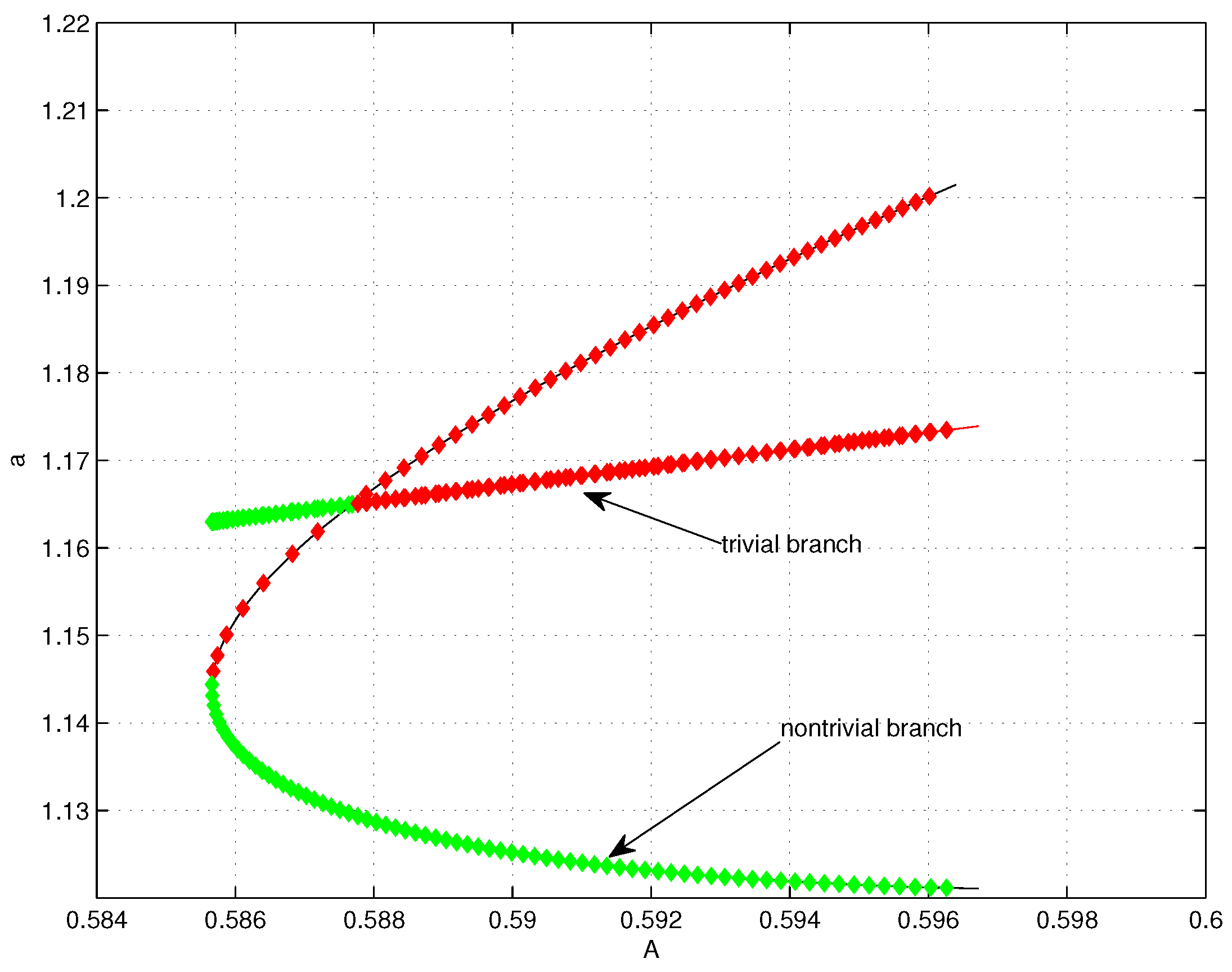
In our first example we consider the Lennard–Jones potential (23) with $c_1=1$, $c_2=2$, ${\delta }_1=12$, and ${\delta }_2=6$. (We obtained similar results for other values of $c_1,c_2$ like those for argon in which $c_1/c_2={3.4}^6$ Å${}^6$.) From equation (24) we get that the bifurcation point off the trivial branch is given approximately by $A_0=0.5877$. For the case of Theorem 3 in which $a=b$, we show in Figure 2 a close-up of the bifurcating branch near this bifurcation point, for the projection onto the A–a plane. In this figure and the others, the color red indicates unstable solutions while the stable ones are marked in green. Please note that the bifurcation is of the trans-critical type. 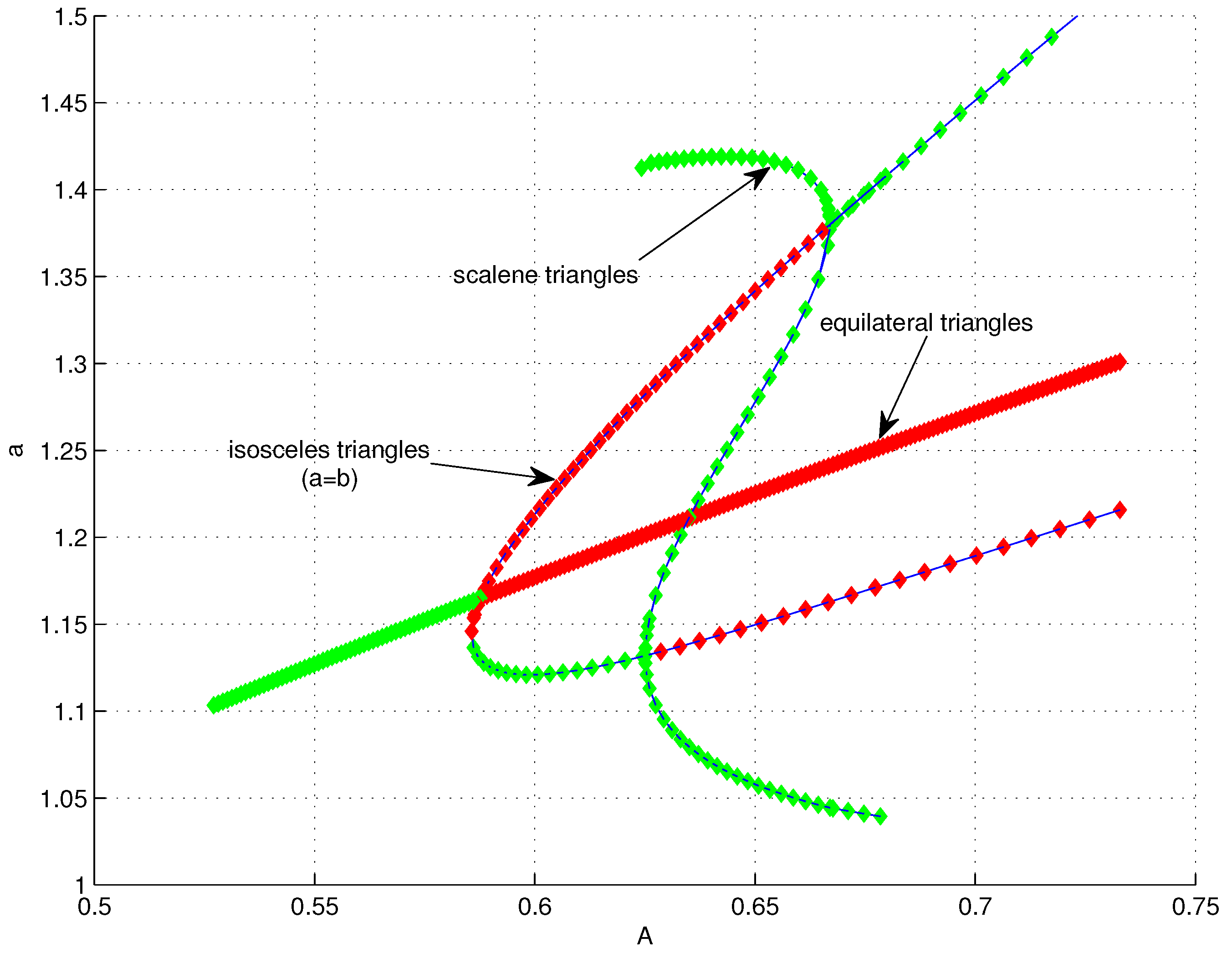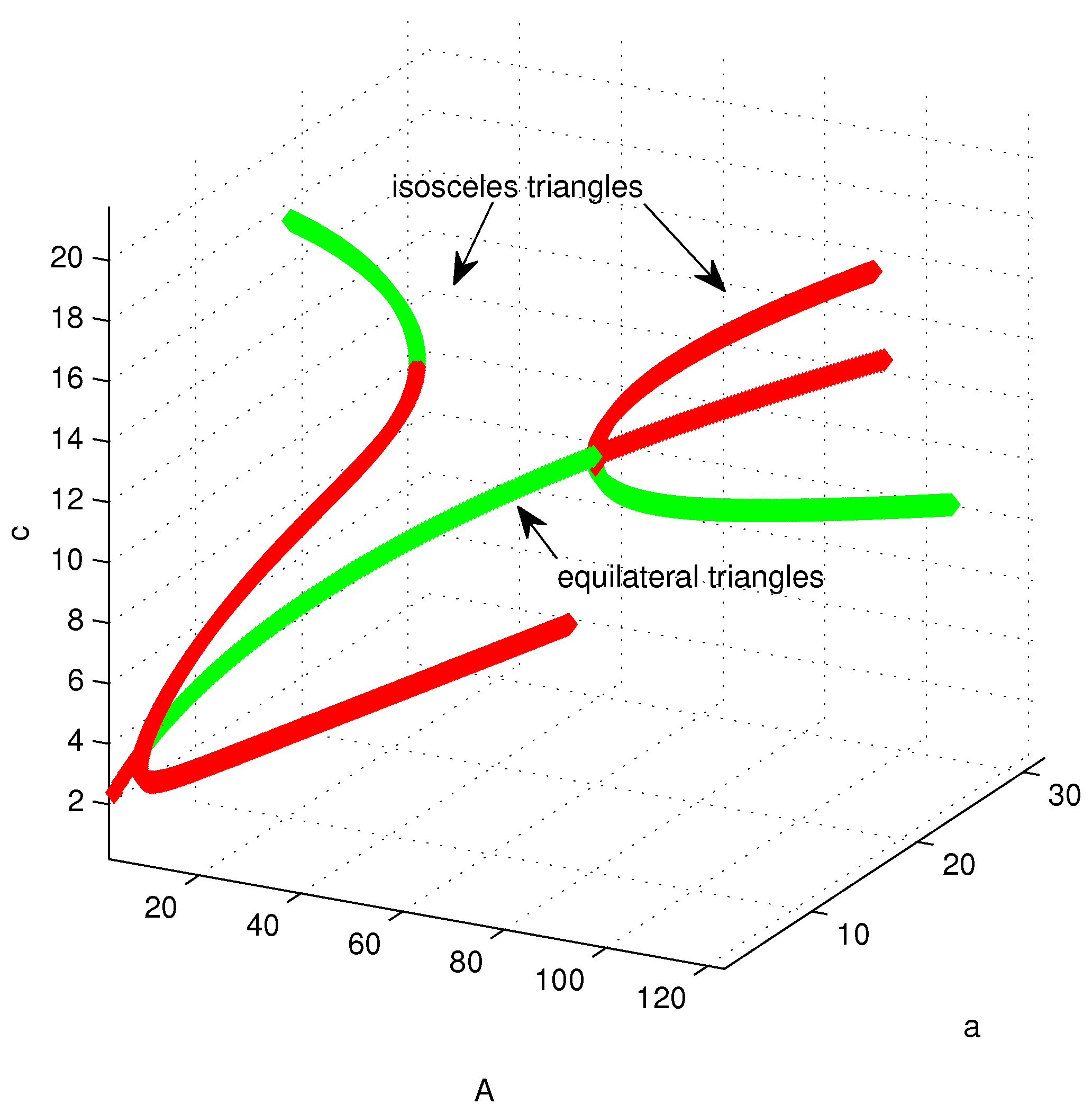It is interesting to note that for an interval of values of the parameter A to the left of $A_0$ in the figure (approximately $(0.5855,0.5877)$), there are multiple states (trivial and nontrivial) which are stable, the trivial one with an energy less than the nontrivial state in this case. In Figure 3 we look at the same branches of solutions, again the projection onto the A–a plane, but for a larger interval of values of A. We now discover that there are two secondary bifurcation points (In Figure 3 there are bifurcations only corresponding to the values of $A_0=0.5877$, $A_1=0.6251$ and $A_2=0.6670$. The apparent crossing of a branch of scalene triangles and the trivial branch is just an artifact of the projection onto the A–a plane.) at approximately $A_1=0.6251$ and $A_2=0.6670$, and once again we have multiple stable states (with different symmetries) existing for an interval of values of the parameter A. The branches of solutions bifurcating at these values of A correspond to stable scalene triangles. 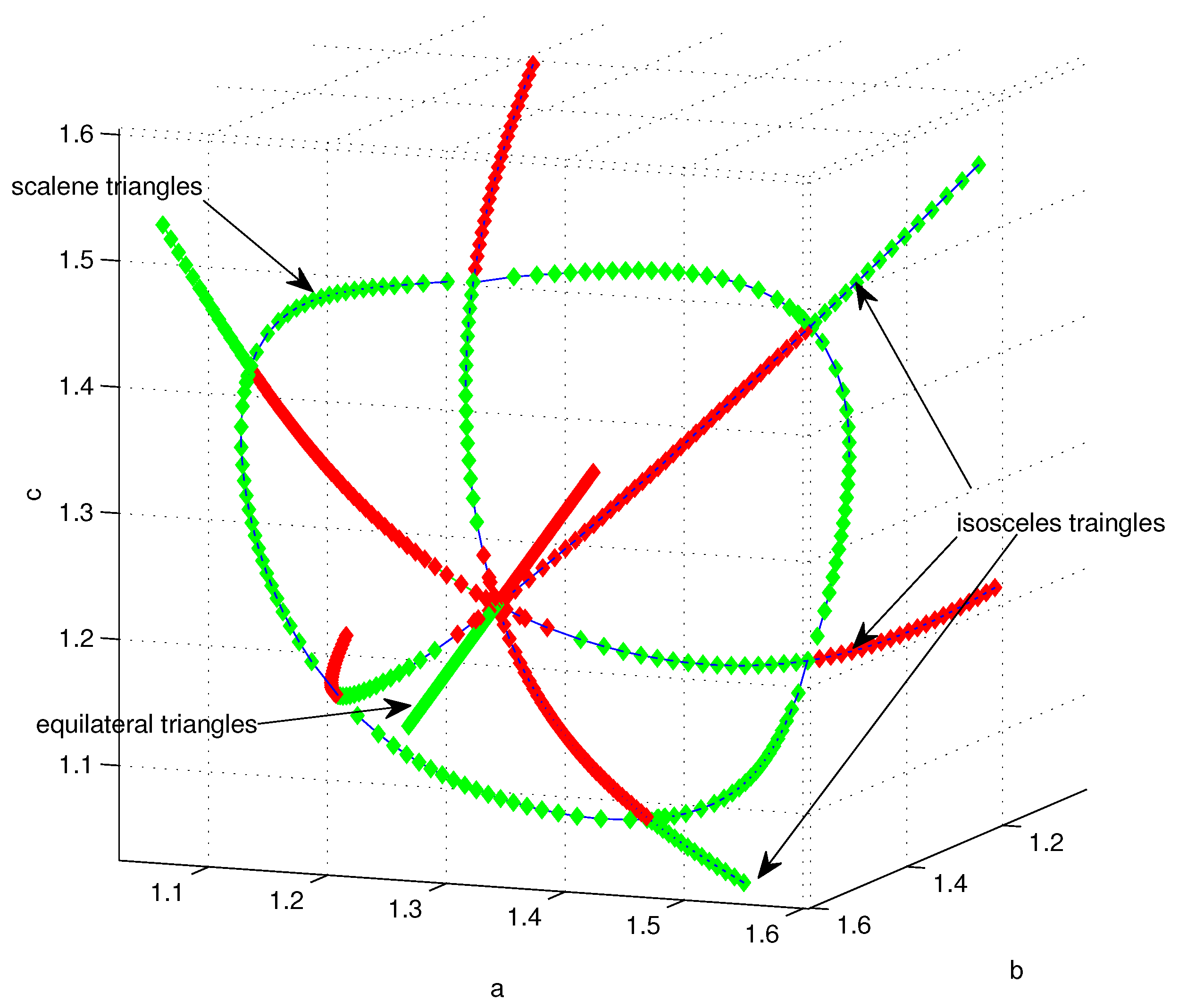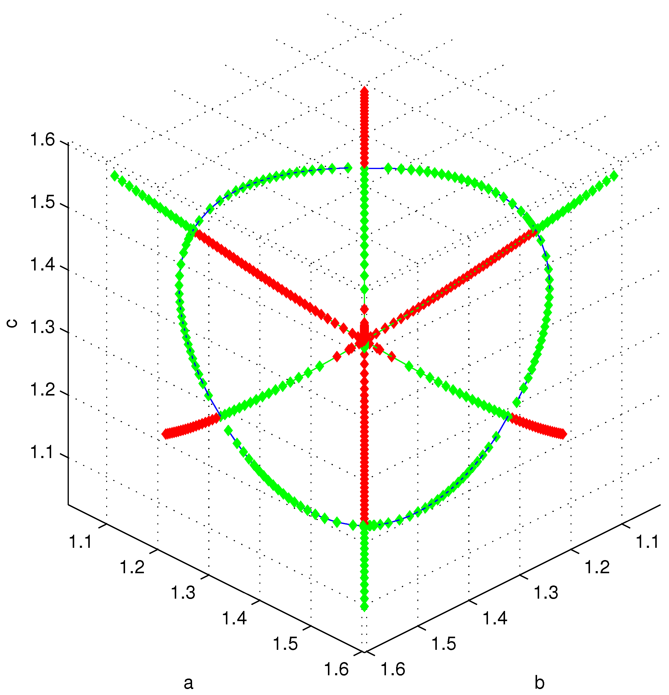Once a branch of solutions is computed, we can use the symmetries (32) to generate other branches of solutions. In Figure 4 we show all the solutions obtained via this process, projected to the $abc$ space (no A dependence). Figure 5 show the same set of solution but with the branch or axis of trivial solutions coming out of the page. The figures clearly show the variety of solutions (stable and unstable) for the problem (12) as well as the rather complexity of the corresponding solution set.

For our next numerical example, we consider the Buckingham potential (25) with parameter values $\alpha =\beta =\gamma =1$ and $\eta =4$, which satisfy (27). In this case, we have two bifurcation points off the trivial branch (which correspond to solutions of $\mu (A)=0$) at approximately $A_0=5.3154$ and $A_1=74.2253$. The trivial branch is stable for $A\in (A_0,A_1)$ and unstable otherwise. Both bifurcations are into isosceles triangles, and both are of trans-critical type but with different stability patterns. In Figure 6 we show the solution set for the case $a=b$. The plot shows the dependence of the a and c components on the area parameter A. 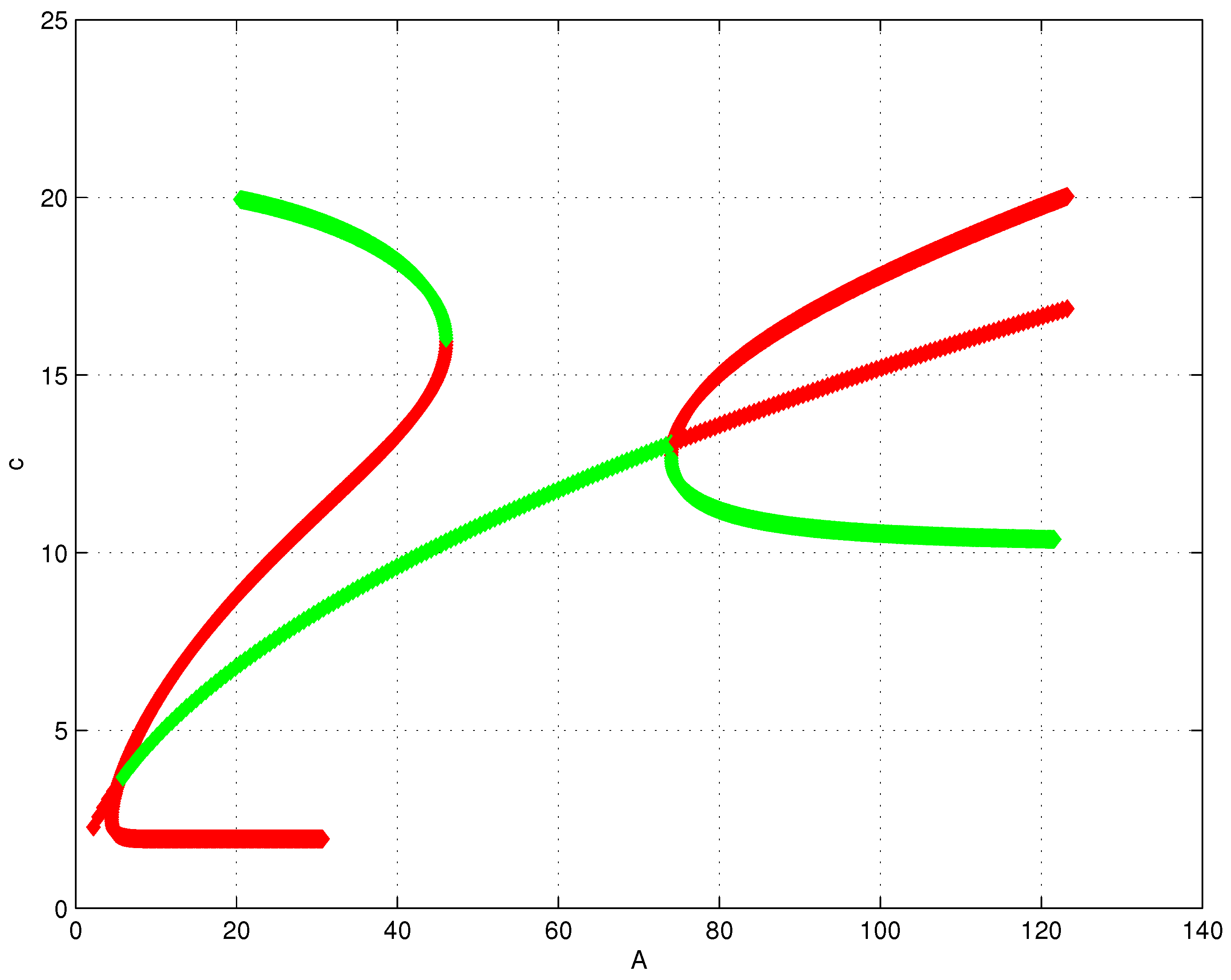In Figure 7 we show the projection of this set onto the c vs. A plane where one can appreciate somewhat better the stability patterns at each bifurcation point, and that there is a turning point for $A\approx 46$ on the branch bifurcating from $A_0$. Please note that once again we have multiple stable states existing for an interval of values of the parameter A. No secondary bifurcations were detected in this case.

6. Final Comments

The variety or type of solutions obtained from Theorems 3, 5–7, could be predicted generically from an analysis of the symmetries present in our problem as given by (32) and (46). However, such an analysis does not guaranty the existence of solutions with the predicted symmetries. It is the application of the Equivariant Bifurcation Theorem 1 that actually yields the result that such solutions exist. The generic analysis however is a preliminary step in identifying the spaces in which Theorem 1 can be applied. We should also point out that the results on the bifurcating branches in Theorems 3, 5–7 are global in the sense that the so-called Crandall and Rabinowitz alternatives in Theorem 1 hold. That is, any bifurcating branch is either unbounded, or it intersects the boundary of the domain of definition of the operator in the equilibrium conditions, or it intersects the trivial branch at another eigenvalue.

The results of this paper might be useful in the analysis of the more general and complex problem of arrays with many particles. As the total area or volume of such an array is increased, thus reducing its density, one might expect that locally situations similar to the ones discussed in this paper might be taking place in different parts of the array. It is interesting to note here that the existence of multiple stable configurations detected in the numerical examples of Section 5, opens the possibility for the existence of multiple equilibrium (local) states in a large molecular array, reminiscent of the bubble formation phenomena mentioned in the introduction. Thus, as further analysis either via molecular dynamics simulations or theoretically would be the questions as to whether the local results in this paper are related or can predict the initiation of cavitation bubbles of different sizes in actual fluid or gases.

References

1. Lim, T.-C. Mathematical relationships for development of a molecular potential function converter. Commun. Math. Comput. Chem. 2003, 49, 155–169. [Google Scholar]
2. Tersoff, J. Modeling solid-state chemistry: Interatomic potentials for multicomponent systems. Phys. Rev. B 1989, 39, 5566–5568. [Google Scholar] [CrossRef]
3. Shang, Y. Lower Bounds for Gaussian Estrada Index of Graphs. Symmetry 2018, 10, 325. [Google Scholar] [CrossRef]
4. Collevecchio, A.; Konig, W.; Morters, P.; Sidorova, N. Phase transitions for dilute particle systems with Lennard-Jones potential. Commun. Math. Phys. 2010, 299, 603–630. [Google Scholar] [CrossRef]
5. Discher, D.E.; Boal, D.H.; Boey, S.K. Phase transitions and anisotropic responses of planar triangular nets under large deformation. Phys. Rev. E 1997, 55, 4762. [Google Scholar] [CrossRef]
6. Golubitsky, M. The Bénard problem, symmetry and the lattice of isotropy subgroups. In Bifurcation Theory, Mechanics and Physics; Bruter, C.P., Aragnol, A., Lichnorowicz, A., Eds.; Reidel: Dordrecht, The Netherlands, 1983; pp. 225–256. [Google Scholar]
7. Bazhirov, T.T.; Norman, G.E.; Stegailov, V.V. Cavitation in liquid metals under negative pressures. Molecular dynamics modeling and simulation. J. Phys. Condens. Matter 2008, 20, 114113. [Google Scholar] [CrossRef]
8. Blander, M.; Katz, J. Bubble Nucleation in Liquids. AlChE J. 1975, 21, 833–848. [Google Scholar] [CrossRef]
9. Fond, C. Cavitation Criterion for Rubber Materials: A Review of Void-Growth Models. J. Polym. Sci. Part B Polym. Phys. 2001, 39, 2081–2096. [Google Scholar] [CrossRef]
10. Horgan, C.O.; Polignone, D.A. Cavitation in nonlinearly elastic solids: A review. Appl. Mech. Rev. 1995, 48, 471–485. [Google Scholar] [CrossRef]
11. Chakraborty, D.; Chandra, A. An analysis of voids and necks in supercritical water. J. Mol. Liquids 2011, 163, 1–6. [Google Scholar] [CrossRef]
12. David, E.E.; David, C.W. Voronoi polyhedra as a tool for studying solvation structure. J. Chem. Phys. 1982, 76, 4611. [Google Scholar] [CrossRef]
13. Lennard-Jones, J.E. On the Determination of Molecular Fields. Proc. R. Soc. Lond. A 1924, 106, 463–477. [Google Scholar]
14. Buckingham, R.A. The classical equation of state of gaseous helium, neon and argon. Proc. R. Soc. Lond. Ser. A Math. Phys. Sci. 1938, 168, 264–283. [Google Scholar] [Green Version]
15. Ambrosetti, A. A Premier on Nonlinear Analysis; Cambridge University Press: Cambridge, UK, 1993. [Google Scholar]
16. Golubitsky, M.; Stewart, I.; Schaeffer, D. Singularities and Groups in Bifurcation Theory: Volume II. In Applied Mathematical Sciences (Book 69); Springer: New York, NY, USA, 2000. [Google Scholar]
17. Kielhöfer, H. Bifurcation Theory: An Introduction with Applications to Pdes; Springer: New York, NY, USA, 2004. [Google Scholar]
18. Krasnoselski, M.A. Topological Methods in the Theory of Nonlinear Integral Equations; Pergamon: Oxford, UK, 1965. [Google Scholar]
19. Healey, T.H. Global bifurcation and continuation in the presence of symmetry with an application to solid mechanics. SIAM J. Math Anal. 1988, 19, 824–840. [Google Scholar] [CrossRef]
20. Wirth, K.; Dreiding, A.S. Edge lengths determining tetrahedrons. Elem. Math. 2009, 64, 160–170. [Google Scholar] [CrossRef]
21. Lim, T.-C. Alignment of Buckingham parameters to generalized Lennard-Jones potential functions. Z. Naturforsch. 2009, 64, 200–204. [Google Scholar] [CrossRef]
22. Shang, Y. Average consensus in multi-agent systems with uncertain topologies and multiple time-varying delays. Linear Algebra Appl. 2014, 459, 411–429. [Google Scholar] [CrossRef]
23. Shang, Y. Couple-group consensus of continuous-time multi-agent systems under Markovian switching topologies. J. Frankl. Inst. 2015, 352, 4826–4844. [Google Scholar] [CrossRef]
24. Keller, H.B. Lectures on Numerical Methods in Bifurcation Problems; Tata Institute of Fundamental Research; Springer: New York, NY, USA, 1986. [Google Scholar]
25. Allgower, E.L.; Georg, K. Introduction to numerical continuation methods. In Classics in Applied Mathematics (Book 45); Society for Industrial and Applied Mathematics: Philadelphia, PA, USA, 2003. [Google Scholar]
Figure 1. Generic graphs of the functions F and G appearing in the stability condition (26) for a Buckingham potential.
Symmetry 11 00158 g001
Figure 2. Bifurcation diagram for the a component vs. A for the system (13) in the case a = b and a Lennard–Jones potential. The points in green represent local minima of (12) while those in red are either maxima or none.
Symmetry 11 00158 g002
Figure 3. Bifurcation diagram for the system (13) in the case of a Lennard–Jones potential for a larger interval of values of A. There are secondary bifurcations into stable scalene triangles.
Symmetry 11 00158 g003
Figure 4. Solution set for the system (13) in the case of a Lennard–Jones potential without the A dependence.
Symmetry 11 00158 g004
Figure 5. Solution set for the system (13) in the case of a Lennard–Jones potential without the A dependence with the branch of trivial solutions coming out of the page.
Symmetry 11 00158 g005
Figure 6. Dependence of the a and c components on the parameter A for the system (13) in the case a = b and for a Buckingham potential.
Symmetry 11 00158 g006
Figure 7. Projection onto the c vs. A plane of the set in Figure 6.
Symmetry 11 00158 g007