Statistical Criteria of Nanofluid Flows over a Stretching Sheet with the Effects of Magnetic Field and Viscous Dissipation

Abstract

In this study, the heat and mass transfer characteristics of nanofluid flow over a nonlinearly stretching sheet are investigated. The important effects of axisymmetric of thermal conductivity and viscous dissipation have been included in the model of nanofluids. The Buongiorno model is considered to solve the nanofluid boundary layer problem. The governing nonlinear partial differential equations have been transformed into a system of ordinary differential equations and are solved numerically via the shooting technique. The validity of this method was verified by comparison with previous work performed for nanofluids without the effects of the magnetic field and viscous dissipation. The analytical investigation is carried out for different governing parameters, namely, the Brownian motion parameter, thermophoresis parameter, magnetic parameter, Biot number, and Eckert number. The results indicate that the skin friction coefficient has a direct relationship with the Brownian motion number and thermophoresis number. Moreover, it can be seen that the Nusselt number decreases with the increase of the magnetic parameter and Eckert number.

1. Introduction

In recent decades, nanofluid technology has contributed to energy costs in terms of heat transfer control in energy systems. Nanoparticles have been used for diverse purposes; for instance, manufacturing and the automotive industry. The external magnetic field effect on nanofluids and fluid flow properties has attracted significant attention due to its applications [1]. Sheikhholeslami et al. [1] studied the radiation of the nanofluid effect in the presence of a magnetic field, and they discovered that the heat transfer rate was reduced with augmentation of Lorentz forces. The magnetic field effect on force convection heat transfer was investigated by Sheikhholeslami et al. [2], who found that the Kelvin force effects are more pronounced at high Reynolds numbers. Turkyilmazoglu [3] investigated the magnetohydrodynamic, electrically conductive slip flow of a non-Newtonian fluid past a shrinking sheet. Their results indicated that the magnetic field presence has considerable effects on temperature and velocity fields. Ishak [4] considered the effects of radiation on the steady two-dimensional magnetohydrodynamic (MHD) flow past a permeable stretching/shrinking sheet. They discovered that the surface rate of heat transfer decreases in the presence of radiation. Sheikholeslami and Kandelousi [5] investigated the spatially variable magnetic field effect on heat transfer and ferrofluid flow by examining the condition of a constant heat flux boundary. They discovered that, as heat transfer increases, the Hartmann number increases and decreases with increases in the Rayleigh and magnetic numbers. The studies of ferrohydrodynamic and MHD effects on convective heat transfer and ferrofluid flow by Sheikholeslami and Ganji [6] demonstrated that the magnetic number results in a dissimilar effect to the Nusselt number. A magnetic field effect on heat transfer and unsteady nanofluid flow has been presented by Sheikholeslami et al. [7] using the Buongiorno model. They showed that there is direct relationship between the coefficient of skin friction with squeeze and the Hartmann number. The magnetic field plays an important role by controlling the cooling rate, which is desired in industrial production. Hence, researchers have studied the flow characteristics over stretching sheets in depth. Considering this situation, Pavlov [8] found that the MHD boundary layer equation gave a similarity solution in exact analytical form. Where in [8] the presence of a uniform transverse magnetic field is considered. The effect of a magnetic field on the viscous flow of an electrically conducting fluid was studied by Hayat et al. [9]. The increasing frictional drag from M = 0 to M = 3 is due to the Lorentz force. Thermal boundary layer becomes thick due to the effect of Lorentz force. Elbashbeshy et al. [10] on their study found that if the magnetic parameter M is increased to M = 2, temperature boundary layer is slightly increased. Results from Noghrehabadi et al. [11] show that the presence of a magnetic field at value M = 3 would significantly affect the boundary layer profiles. An increase in magnetic parameter from M = 0.1 to M = 3 would decrease the reduced Nusselt and Sherwood numbers. The magnetic field at M = 5 strongly affects the velocity and consequently temperature profiles; the effect of magnetic field is negligible on the thickness of the boundary layer. Elbashbeshy and Aldawody [12] also found that the local Nusselt number decreases when the magnetic parameter M = 0.4.

Yasin et al. [13] considered the effects of radiation on the steady two-dimensional magnetohydrodynamic (MHD) flow past a permeable stretching/shrinking sheet. They discovered that the surface rate of heat transfer decreases in the presence of radiation. Pal et al. [14] analyzed the thermal radiation effect on hydromagnetic mixed convection flow over nonlinear shrinking/stretching sheets in nanofluids. They discovered that copper–water nanofluids have a higher rate of mass transfer in contrast with titanium dioxide—water and alumina—water nanofluids. Many researchers have concentrated on the improvement of heat transfer by altering nanoparticles in base fluids. This has been used in photonics, transportation, and electronics [15,16,17,18,19]. Nanoparticles in a base fluid are found to have better convective heat transfer coefficients and thermal conductivity than with the base fluid [20,21,22,23,24,25,26,27,28]. Based on these observations, the objective of this study is to analyze the effect of the thermal radiation, viscous dissipation, and thermal convective boundary condition on the flow of nanofluids over a nonlinear stretching sheet. From the examined literature, the problem of the effect of the magnetic field and viscous dissipation with a thermal convective boundary condition has not been discussed. We aim, in the present paper, to analyze the effect of the magnetic field and viscous dissipation over a stretching sheet using the Runge–Kutta–Fehlberg method with the shooting technique. The effects of governing parameters are analyzed based on fluid velocity, temperature, and particle concentration. The results are then shown graphically and also in tables. The available results in the literature are then compared with the results found in this study. Excellent agreement is found for both comparisons.

2. Problem Formulation

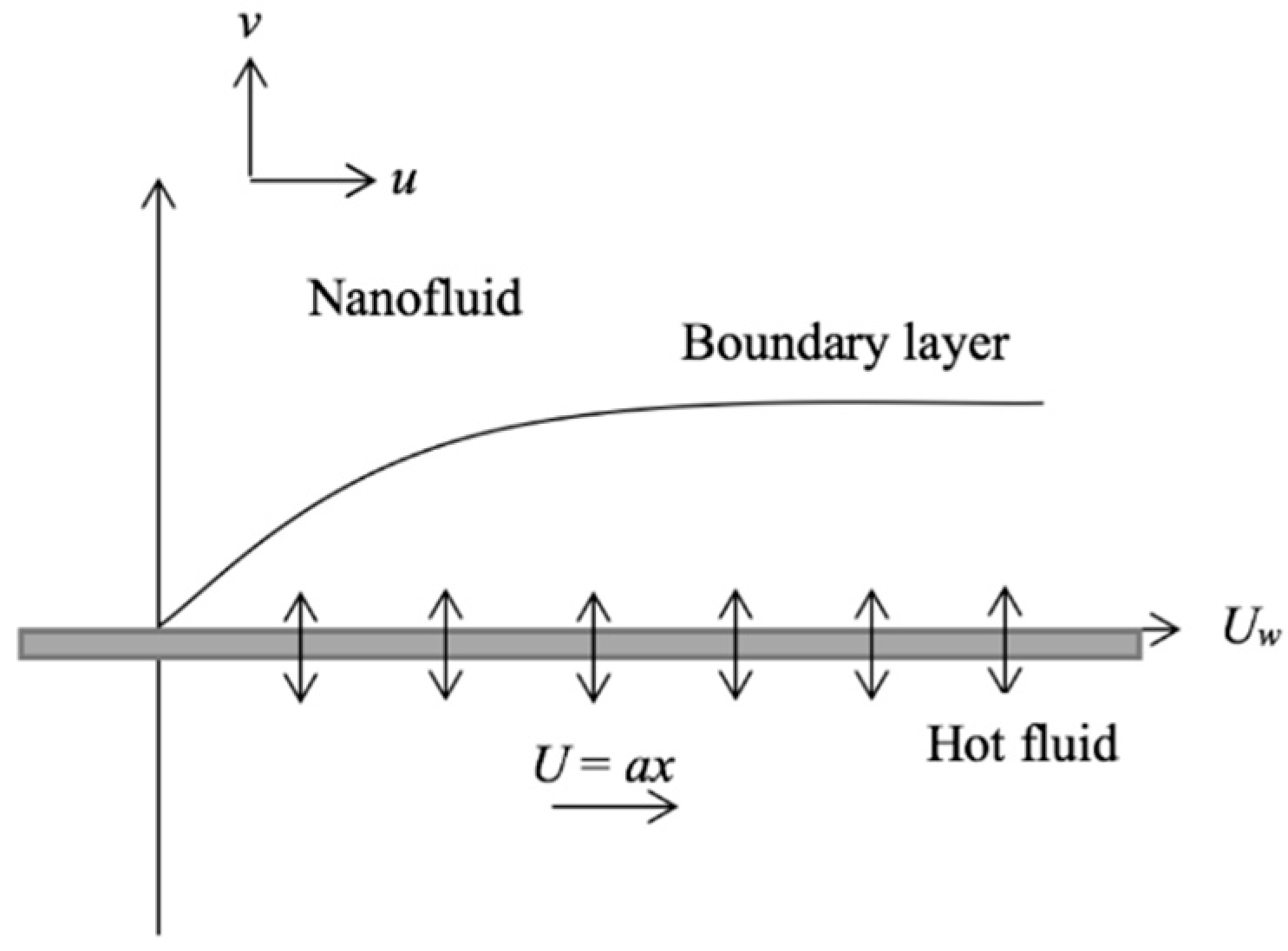
Consider a steady axisymmetric thermal conductivity, laminar, incompressible, and one-dimensional flow in a nanofluid towards a permeable stretching sheet is placed on the plane y = 0, where y and x are Cartesian coordinates estimated along the stretching surface and typical of it, respectively. The flow is limited at y > 0. The sheet is extended with a speed U_w = ax along the x-direction while assuming the pressure gradient and external force to be zero, where a is a positive constant value. Further, we assume that the flat plate is heated from below by a hot fluid whose temperature is T_f, with a heat transfer coefficient h_f. The scheme of the physical configuration is depicted in Figure 1.

Using boundary layer approximations, the final steady momentum, energy, continuity, and nanoparticle concentration equations are defined as below (see Zaimi et al. [23]):

$$\frac{\partial u}{\partial x}+\frac{\partial v}{\partial y}=0,$$

(1)

$$u\frac{\partial u}{\partial x}+v\frac{\partial u}{\partial y}=\nu \frac{{\partial }^{2}u}{\partial y^2}-\frac{\gamma B^2\left(x\right)}{{\rho }_f}\cdot u,$$

(2)

$$u\frac{\partial v}{\partial x}+v\frac{\partial v}{\partial y}=-\frac{1}{\rho }\frac{\partial \rho }{\partial y}+\nu \frac{{\partial }^{2}v}{\partial y^2}-\frac{\gamma B^2\left(x\right)}{{\rho }_f}\cdot u,$$

(3)

$$u\frac{\partial T}{\partial x}+v\frac{\partial T}{\partial y}=\alpha \frac{{\partial }^{2}T}{\partial y^2}+\tau \left[D_B\frac{\partial C}{\partial y}\frac{\partial T}{\partial y}+\frac{D_T}{T_{\infty }}{\left(\frac{\partial T}{\partial y}\right)}^2\right]+\frac{D_m{K}_T}{c_s{c}_p}\frac{{\partial }^{2}C}{\partial y^2}+\frac{V}{c_p}{\left(\frac{\partial u}{\partial y}\right)}^2,$$

(4)

$$u\frac{\partial C}{\partial x}+v\frac{\partial C}{\partial y}=D_B\frac{{\partial }^{2}C}{\partial y^2}+\frac{D_T}{T_{\infty }}\frac{{\partial }^{2}T}{\partial y^2}+\frac{D_m{K}_T}{T_m}\frac{{\partial }^{2}T}{\partial y^2},$$

(5)

referring to the initial boundary conditions

$$\begin{array}{l}u=U+N\rho \nu \left(\frac{\partial u}{\partial y}\right),v=v_w,-k\left(\frac{\partial T}{\partial y}\right)=h_f\left(T_f-T\right),C=C_w\mathrm{at}y=0,\\ u\to 0,T\to T_{\infty },C\to C_{\infty }\mathrm{as}y\to \infty \end{array}$$

(6)

where v and u are the corresponding velocity components in the y and x directions, respectively. In Equation (3) by using the scaling analysis, the pressure gradient ∂p/∂y can be ignored because the pressure change across the thickness of boundary layer is negligible. Therefore, the Equation (3) is neglected so that the momentum Equation (2) is considered as one-dimensional. For the next part, we identify the temperature in the boundary layer (T) and ambient temperature T_∞, where C is the nanoparticle concentration in the boundary layer, C_w is the nanoparticle volume fraction at the plate, T_w is the surface temperature, C_∞ is the nanoparticle volume fraction far from the plate, $\nu$ represents the coefficient of kinematic viscosity, D_B is the coefficient of Brownian diffusion, D_T is the coefficient of thermophoresis diffusion, $\alpha =k/{\left(\rho c\right)}_f$ is the fluid thermal diffusivity, $\gamma$ is electrical conductivity, $\tau ={\left(\rho c\right)}_p/{\left(\rho c\right)}_f$ is the ratio between the effective heat capacity of the nanoparticle material and the heat capacity of the fluid,${\rho }_p$ is the particle density,${\rho }_f$ is the fluid density, D_B is the Brownian diffusion coefficient, c is the volumetric volume expansion coefficient, $K_T$ is the thermal diffusion ratio, D_T is the thermophoresis diffusion coefficient, D_B is the Brownian diffusion coefficient, D_m is the coefficient of mass diffusivity, Kn is the Knudsen number, T_m is the mean fluid temperature, c_s is the concentration susceptibility, c_p is the specific heat at constant pressure, $N\rho \nu$ is the velocity slip factor, v_w is the suction or injection velocity with v_w > 0 for suction and v_w < 0 for injection, and $\epsilon$ is the stretching/shrinking parameter with $\epsilon >0$ for a stretching case and $\epsilon <0$ for a shrinking case. The constant n is the nonlinearity parameter with n = 1 for the linear case and $n\ne 1$ for the nonlinear case. We assume that the variable magnetic field B (x) = B₀ x^(n−1)/2. A flow with a coefficient of convective heat transfer h_f as well as temperature of T_f moves through the stretching surface. The plate and the fluid have a slippery surface, upon which the length of slip will be created; this length is important for enhancing the heat transfer rate and widening the range of possible dual solutions. In a recent study, we investigated the relations between the effects of the partial slip and the thermal convective boundary condition towards the performance of the heat and mass transfer rate. Moreover, in finding dual solutions, this study needs to consider a permeable surface where the suction is presented to allow the movement of nanoparticles and fluid. By considering the nanofluid model of Buongiorno [25], we assume that the nanofluid’s relative motion is caused by Brownian motion and thermophoresis but only in the case of general nanoparticles and fluid base; i.e., size, nature, concentration.

We now introduce the following dimensionless variables:

$$\begin{array}{l}u=a{x}^n{f}^{\prime }\left(\eta \right),v=-{\left(\frac{av\left(n+1\right)}{2}\right)}^{1/2}\left[f^{\prime }\left(\eta \right)+\frac{n-1}{n+1}\eta f^{\prime }\left(\eta \right)\right],\\ \eta =y{\left(\frac{av\left(n+1\right)}{2v}\right)}^{1/2}{x}^{\left(n-1\right)/2},\theta \left(\eta \right)=\frac{T-T_{\infty }}{T_f-T_{\infty }},\varphi \left(\eta \right)=\frac{C-C_{\infty }}{C_w-C_{\infty }},\end{array}$$

(7)

where $\eta$ is the similarity variable. Moreover, $\varphi \left(\eta \right)$, $f\left(\eta \right)$, and $\theta \left(\eta \right)$ are the dimensionless nanofluid concentration, velocity, and temperature in the boundary layer region, respectively. A nonlinear equation is written as axⁿ, where n is the number of degrees, and a is constant. By introducing the relation (7) into the Equations (2) to (5), we obtain the following nonlinear ordinary differential equations.

$$f^{‴}+f{f}^{″}-\frac{2n}{n+1}{f^{\prime }}^2-M·f^{\prime }=0,$$

(8)

$$\frac{1}{\mathrm{Pr}}{\theta }^{″}+f{\theta }^{\prime }+Nb{\theta }^{\prime }{\varphi }^{\prime }+Nt{{\theta }^{\prime }}^2+Du{\varphi }^{″}+Ec{f^{″}}^2=0,$$

(9)

$${\varphi }^{″}+Lef{\varphi }^{\prime }+\frac{Nt}{Nb}{\theta }^{″}+SrLe{\theta }^{″}=0,$$

(10)

where prime denotes the differentiation with respect to $\eta$. Further, Nb is the Brownian motion parameter, M is the magnetic parameter, Pr is the Prandtl number, Nt is the thermophoresis parameter, Ec is the Eckert number, Du is the Dufour number, Sr is the Soret number, and Le is the Lewis number. The boundary conditions are now transformed to

$$\begin{array}{l}f\left(0\right)=S,f^{\prime }\left(0\right)=1+\sigma f^{″}\left(0\right),{\theta }^{\prime }\left(0\right)=Bi\left(\theta -1\right),\varphi \left(0\right)=1,\\ f^{\prime }\left(\eta \right)\to 0,\theta \left(\eta \right)\to 0,\varphi \left(0\right)\to 0\mathrm{as}\eta \to \infty ,\end{array}$$

(11)

With

$$v_w=-{\left(\frac{av\left(n+1\right)}{2v}\right)}^{1/2}{x}^{\left(n-1\right)/2}S,$$

(12)

where S is known as the constant mass transfer parameter, with $S<0$ corresponding to mass injection and $S>0$ corresponding to mass suction. Next, $\sigma$ is the velocity slip parameter, and Bi is the second-order velocity slip parameter or Biot number. The parameters are composed as follows:

$$\sigma =N\rho \nu a{x}^{\left(2n-1\right)/2}{\left(\frac{a\left(n+1\right)}{2v}\right)}^{1/2},Bi=\frac{h_f}{k}{\left(\frac{u}{v_w}\right)}^{1/2}$$

(13)

The other parameters are written as

$$\begin{array}{l}\mathrm{Pr}=\frac{\nu }{\alpha },Le=\frac{\nu }{D_B},Nb=\frac{{\left(\rho c\right)}_p{D}_B\left(C_w-C_{\infty }\right)}{{\left(\rho c\right)}_f\nu },Nt=\frac{{\left(\rho c\right)}_p{D}_T\left(T_f-T_{\infty }\right)}{{\left(\rho c\right)}_f{T}_{\infty }\nu }\\ Du=\frac{D_m{K}_T\left(C_w-C_{\infty }\right)}{c_s{c}_p\nu \left(T_f-T_{\infty }\right)},Sr=\frac{D_m{K}_T\left(T_f-T_{\infty }\right)}{\nu T_m\left(C_w-C_{\infty }\right)},\\ Ec=\frac{u^2}{c_p\left(T_w-T_{\infty }\right)},M=\frac{2\sigma B{i}^2}{\alpha {\rho }_f\left(n+1\right)}\end{array}$$

(14)

where Le is the Lewis number, Pr is the Prandtl number, Nt is the thermophoresis parameter, Nb is the Brownian motion parameter, Sr is the Soret number, Du is the Dufour number, M is the magnetic parameter, and Ec is the Eckert number.

The physical quantities of interest are the local Nusselt number $N{u}_x$, skin friction coefficient $C_f$, and local Sherwood number $S{h}_x$, known as

$$C_f=\frac{{\tau }_w}{\rho {U_{\infty }}^2},N{u}_x=\frac{x{q}_w}{k\left(T_f-T_{\infty }\right)},S{h}_x=\frac{x{q}_m}{D_B\left(C_w-C_{\infty }\right)},$$

(15)

where the local heat flux $q_w$, stress of wall shear ${\tau }_w$, as well as the local mass flux $q_m$ are defined as follows:

$${\tau }_w=\mu {\left(\frac{\partial u}{\partial y}\right)}_{y=0},q_w=-k{\left(\frac{\partial T}{\partial y}\right)}_{y=0},q_m=-D_B{\left(\frac{\partial T}{\partial y}\right)}_{y=0},$$

(16)

where $\mu$ is the dynamic viscosity of the nanofluids, and k is the thermal conductivity of the nanofluids, and k is taken to be a constant nonisotropic axisymmetric tensor of thermal conductivity.

Using the similarity variables (7), the local Nusselt number, local Sherwood number, and reduced skin friction coefficient are

$$C_f{{\mathrm{Re}}_x}^{1/2}=f^{″}\left(0\right),N{u}_x{{\mathrm{Re}}_x}^{-1/2}=-{\theta }^{\prime }\left(0\right),S{h}_x{{\mathrm{Re}}_x}^{-1/2}=-{\varphi }^{\prime }\left(0\right),$$

(17)

where ${\mathrm{Re}}_x=U_{\infty }x/\nu$ is the local Reynolds number.

Using dimensional analysis, the function of the Reynolds and Schmidt numbers is expressed by the Froessling equation:

$$Sh=S{h}_0+C{\mathrm{Re}}^{1/2}S{c}^{1/3}$$

(18)

where Sh₀ is the Sherwood number due only to natural convection and not forced convection while C is a constant. Regarding Equation (15), the Sherwood numbers are calculated with several parameters dependent on the concentration. Sherwood numbers are shown for different Ec, Bi, Nb, Nt, and M values according to Equation (18).

3. Results and Discussion

The flow, mass, and heat transfer on a stretching sheet with magnetic, partial slip, Eckert, and Biot effects were analyzed. Using the shooting method, we solved ordinary differential system Equations (8) to (10) subject to boundary conditions (11). This method is stated by Torrance and Jaluria in their book [24] and has been applied extensively in the present work; see Salleh et al. [25]. Using this method, dual solutions were obtained by employing various initial guesses for unknown values of the reduced local Nusselt number $-{\theta }^{\prime }\left(0\right)$, reduced local Sherwood number $-{\varphi }^{\prime }\left(0\right)$, and reduced skin friction coefficient $f^{″}\left(0\right)$, where the infinity boundary conditions are satisfied by all the temperature, velocity, and nanoparticle concentrations (11) asymptotically but with different boundary layer thicknesses and shapes.

Table 1. The reduced local Nusselt number $-{\theta }^{\prime }\left(0\right)$ with effects of σ and $\epsilon$. (Nb = 0.5, Nt = 0.5, Le = 2, S = 2.5, n = 2, Pr = 1, σ = 0.1, Sr = 0.1, Du = 0.5).

σ	ε	$-{\mathit{\theta }}^{\prime }\left(0\right)$
		Zaimi et al. [23]	Present Results M = 0, Ec = 0, and Bi = 0	Present Results M = 0.1, Ec = 0.1, and Bi = 0.1
0.1	−1	1.4298738 [1.5108520]	1.4298738 [1.5108520]	1.5132575 [1.3789473]
	−0.5	-	1.4586293 [1.5716212]	1.5839247 [1.4452501]
	0	1.4850957 [1.6068106]	1.4850957 [1.6068106]	1.5957988 [1.4850957]
	0.5	-	1.5096806 [1.6326134]	1.5630076 [1.4951495]
1	−1	1.4657975 [1.5215138]	1.4657975 [1.5215138]	1.5206108 [1.4588067]
	−0.5	-	1.4757430 [1.5499348]	1.5577777 [1.4740737]
	0	1.4850957 [1.5716768]	1.4850957 [1.5716768]	1.5817981 [1.4850957]
	0.5	-	1.4939579 [1.5879273]	1.5940551 [1.4921329]
	1	1.5024036 [1.60007110]	1.5024036 [1.60007110]	1.5973980 [1.4953789]

[ ] second solution.

shows a comparison of previous results with the local Nusselt number [23] in the absence of partial slip and magnetic, Eckert, and Biot effects as a benchmark, showing that the numerical results are in perfect agreement. We assume M = 0, Ec = 0, and Bi = 0 so that the values of the reduced local Nusselt number are similar with those in [23] by using similar shooting method. Comparison are also made using M = 0.1, Ec = 0.1, and Bi = 0.1, and it is found that the present results in Table 1 show the values of local Nusselt number is higher than [23]. The numerical values of some important physical quantities are presented in

Table 2. Values $f^{″}\left(0\right)$, $-{\theta }^{\prime }\left(0\right)$, and $-{\varphi }^{\prime }\left(0\right)$ with Bi, M, Ec, and $\epsilon$ when Nb = 0.5, Nt = 0.5, Sr = 0.1, Du = 0.1, Pr = 1, S = 2.5, $\sigma$ = 0.1, n = 2, and Le = 2.

Bi	M	Ec	ε	${\mathit{f}}^{″}\left(0\right)$	$-{\mathit{\theta }}^{\prime }\left(0\right)$	$-{\mathit{\varphi }}^{\prime }\left(0\right)$
0.1	0.2	0.1	1	−2.2391822	0.0815095	2.4485787
				[−3.7001711]	[0.0706781]	[1.7947827]
				−1.0756013	0.0838298	2.4521358
				[−2.5565807]	[0.0759208]	[1.8890286]
			0	1.2279546	0.0844259	2.3986889
				[−1.5382880]	[0.0790001]	[1.8908379]
	0.1	0.2	1	−2.2208376	0.0781744	2.3545960
				[−3.6428921]	[0.0597493]	[1.4806476]
			0.5	−1.0652139	0.0830049	2.4294086
				[−2.5002446]	[0.07057078]	[1.7555915]
			0	0	0.0844259	2.3986889
				[−1.4795582]	[0.0771729]	[1.8760263]
1	0.2	0.1	1	−2.2391822	0.5819357	1.8647797
				[−3.7001711]	[0.4988329]	[1.1832779]
			0.5	−1.0756013	0.5950489	1.8480621
				[−2.5565807]	[0.5315346]	[1.2200802]
			0	1.2279461	0.5950033	1.7859959
				[−1.5382880]	[0.5474027]	[1.1766139]
	0.1	0.2	1	−2.2208376	0.5577470	1.7953111
				[−3.6428921]	[0.4218679]	[0.9766738]
			0.5	−1.0652139	0.5891219	1.8315048
				[−2.5002447]	[0.4946099]	[1.1522619]
			0	0	0.5950033	1.7859959
				[−1.4795582]	[0.5356944]	[1.2030547]

[ ] second solution.

. Different governing nondimensional parameters effect are discussed, namely, the Brownian motion parameter Nb, Prandtl number Pr, thermophoresis parameter Nt, Dufour number Du, Soret number Sr, magnetic number M, Eckert number Ec, Biot number Bi, Lewis number Le, mass suction parameter S, velocity slip parameter $\sigma$, stretching parameter $\epsilon$, and nonlinearity parameter n. We assumed constant values for several parameters, which are Pr = 1, Nb = 0.5, Nt = 0.5, Sr = 0.1, Du = 0.1, S = 2.5, $\sigma$ = 0.1, n = 2, and Le = 2. The values of parameters are based on the behavior of velocity, temperature, and nanoparticle concentration profiles to ensure the figures move asymptotically in the x-axis. Besides his, the chosen of the value of suction S > 2 is important to obtain dual solutions.

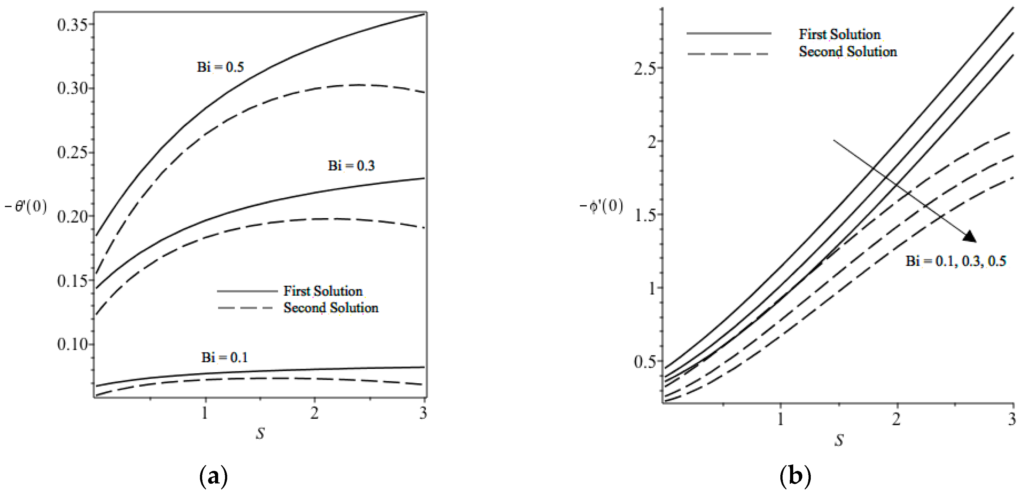
The results of the reduced local Nusselt number $-{\theta }^{\prime }\left(0\right)$ as well as the reduced local Sherwood number $-{\varphi }^{\prime }\left(0\right)$ variation with the parameter of mass suction S for Bi = 0.1, 0.3, and 0.5 when Le = 2, Pr = 1, Nb = 0.5, Nt = 0.5, $\sigma$ = 0.1, n = 2, Du = 0.2, Sr = 0.1, M = 0.1, and Ec = 0.1 for a stretching surface ($\epsilon$ = 1) are shown in Figure 2a,b, respectively. From these figures, when the Bi increases, the values of $-{\theta }^{\prime }\left(0\right)$ increases; meanwhile, the value of $-{\varphi }^{\prime }\left(0\right)$ decreases. Figure 2a indicates that the dimensionless heat transfer rate increases with mass suction S and the Biot number. Physically, this can be attributed to the increase of temperature gradient with respect to mass suction and the Biot number. However, the perplexing results obtained in Figure 2b show that the dimensionless mass transfer rate decreases when the Biot number increases. The impact of suction on the rate of mass transfer, as shown in Figure 2b, is evidence that the rate of mass transfer reduces with an increase in the Biot and suction values.

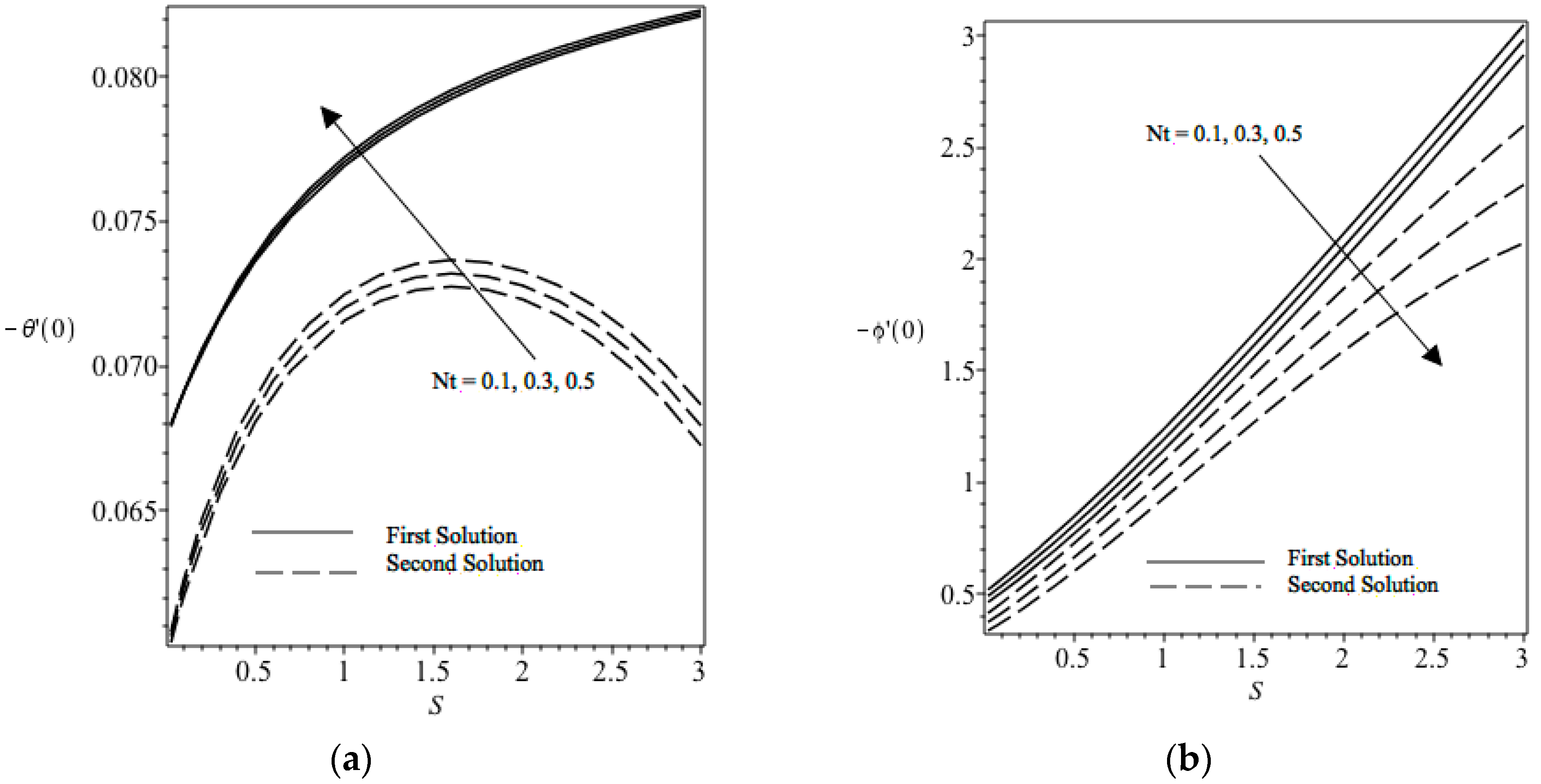
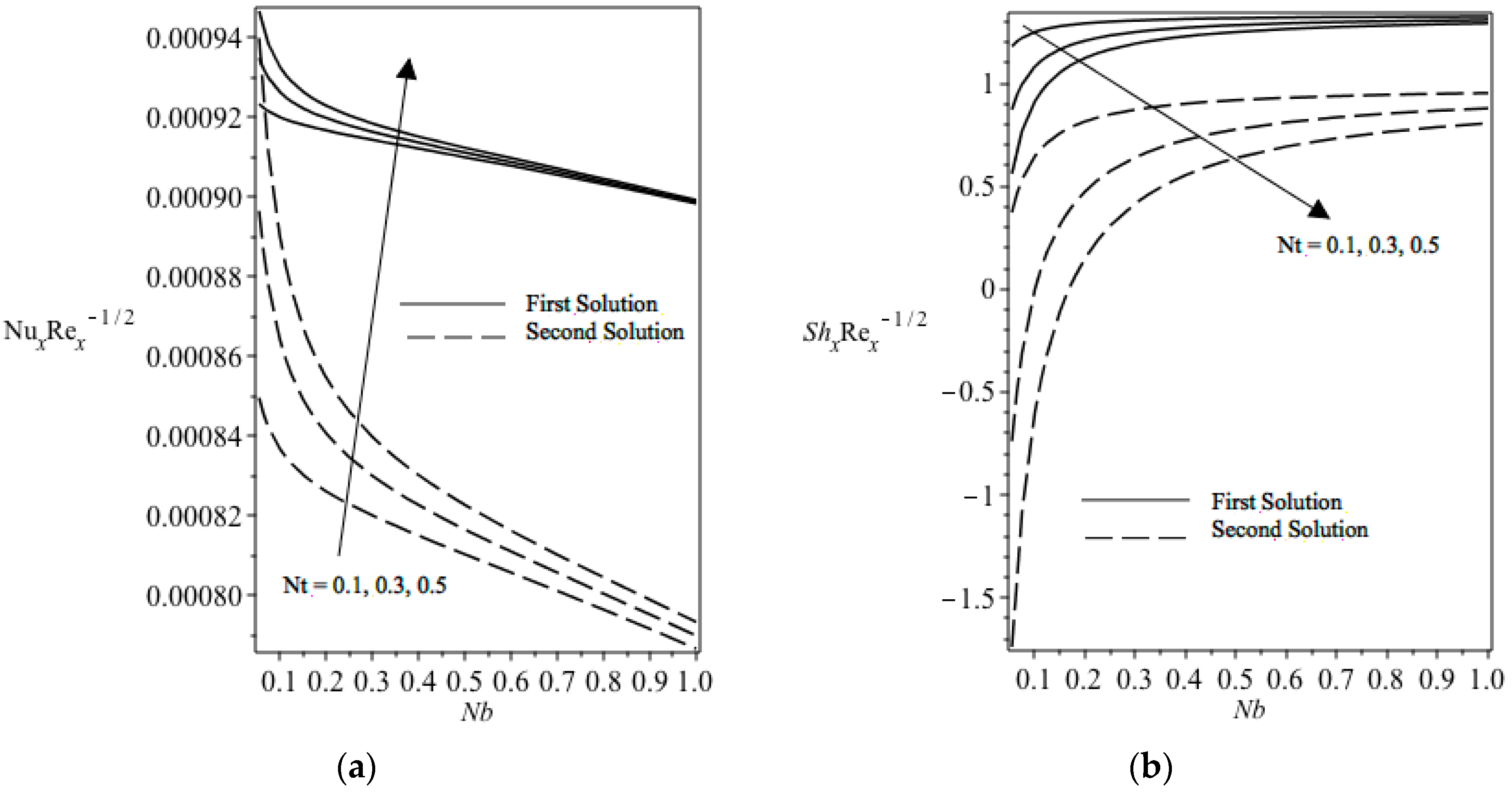
Figure 3a,b demonstrates the values of the reduced local Nusselt number $-{\theta }^{\prime \left(0\right)}$ and reduced local Sherwood number $-{\varphi }^{\prime }\left(0\right)$, respectively, for the stretching case ($\epsilon$ = 1) for several thermophoresis parameter values, Nt = 0.1, Nt = 0.3, and Nt = 0.5 when Le = 2, Pr = 1, Nb = 0.5, Bi = 0.1, $\sigma$ = 0.1, n = 2, Du = 0.2, Sr = 0.1, M = 0.1, and Ec = 0.1. From Figure 3a, it is seen that as Nt increases, the heat transfer rates increase and, thus, the thermal boundary layer thickness decreases. As the boundary layer thickness decreases, the temperature gradient at the surface increases. However, Figure 3b shows that a smaller Nt is enough to increase transfer rates. This is due to the fact that the thermal boundary layer thickness will increase once Nt is intensified. As the thermal boundary layer thickness increases, we can expect that the temperature gradient at the surface grows smaller. Thus, the local Sherwood number decreases. Increasing S values will increase the mass and heat transfer rate, as shown in Figure 3a,b, respectively.

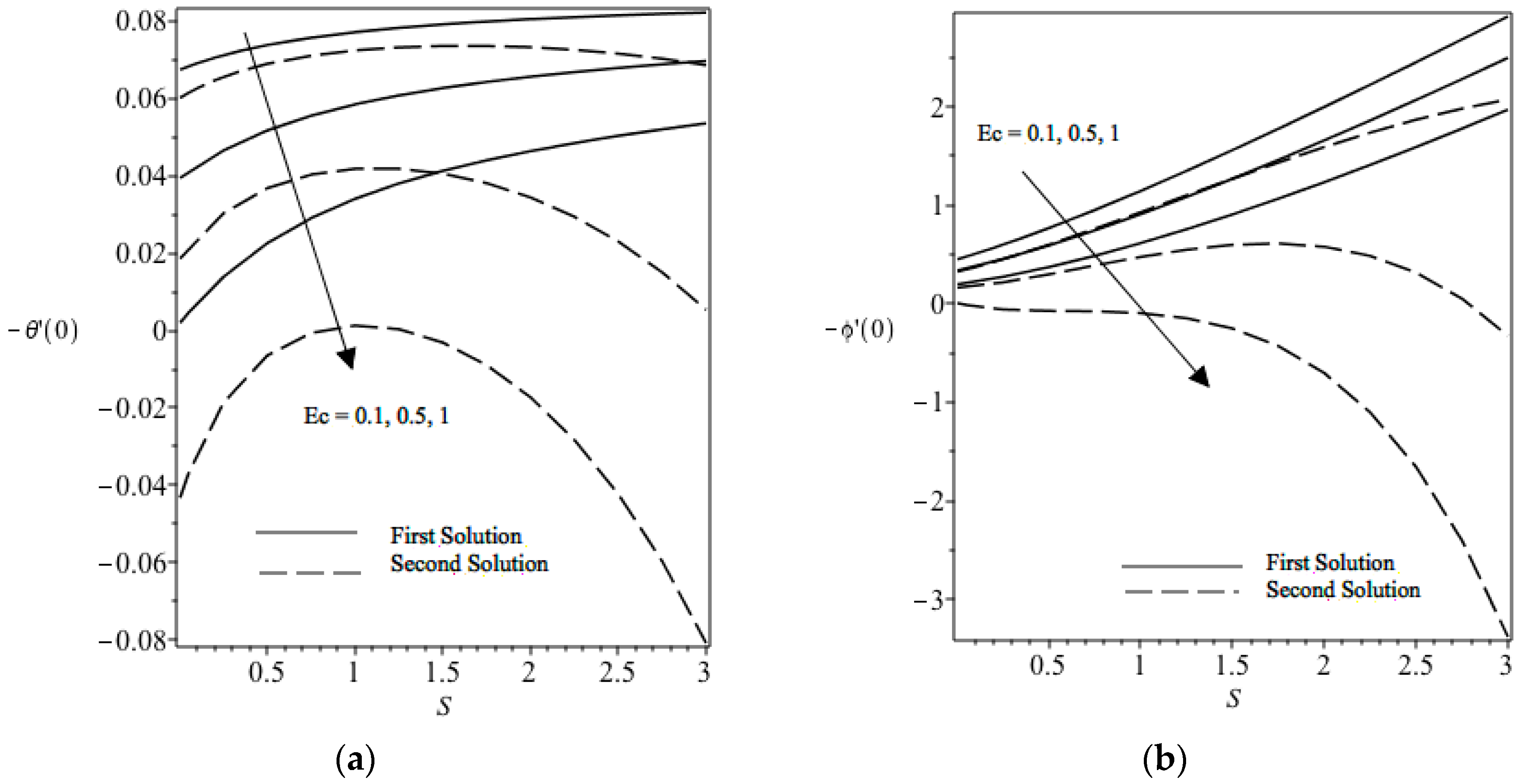
Figure 4a,b depicts the reduced local Nusselt number $-{\theta }^{\prime }\left(0\right)$ as well as reduced local Sherwood number $-{\varphi }^{\prime }\left(0\right)$ variation, respectively, for a stretching case for various values of Eckert Ec with other fixed value parameters (Pr = 1, Le = 2, Nt = 0.5, Nb = 0.5, Bi = 0.1, $\sigma$ = 0.1, n = 2, Du = 0.2, Sr = 0.1, M = 0.1, and S = 2.5). From Figure 4a,b, it is clearly seen that the decreasing Eckert number increases the rate of mass and heat transfer, respectively. The effect of the Eckert number (Ec) is negligible when there is greater suction. It is also shown that as the Eckert number (Ec) increases, the local Nusselt number $-{\theta }^{\prime }\left(0\right)$ and local Sherwood number $-{\varphi }^{\prime }\left(0\right)$ will decrease; hence, it is prone to increasing the nanoparticle and thermal boundary layer thicknesses.

Figure 5a portrays the local Nusselt number variation with the Brownian motion parameter (Nb) for some thermophoresis parameter Nt values when stretching is considered; meanwhile, the corresponding local Sherwood number is illustrated in Figure 5b. For Figure 5a,b, other parameters are fixed (Le = 2, Pr = 1, Nb = 0.5, Bi = 0.1, $\sigma$ = 0.1, n = 2, Du = 0.2, Sr = 0.1, Ec = 0.1, M = 0.1, and S = 2.5). From Figure 5a, it is clearly shown that when Nb increases, the local Nusselt number gradually decreases, while it increases along with increasing Nt; thus, it will cause a decrease in thermal boundary layer thickness. Figure 5b demonstrates that the increasing of thermophoresis Nt decreases the mass transfer rate; in other words, the ratio of the convective mass transfer to the mass diffusivity becomes smaller. This is due to the lager values of Nt where the viscosity of the base fluid is strong and has tendency for nanoparticles to move among themselves less easily. This phenomenon makes the fluid to cool slower and therefore the heat transfer rate decreases.

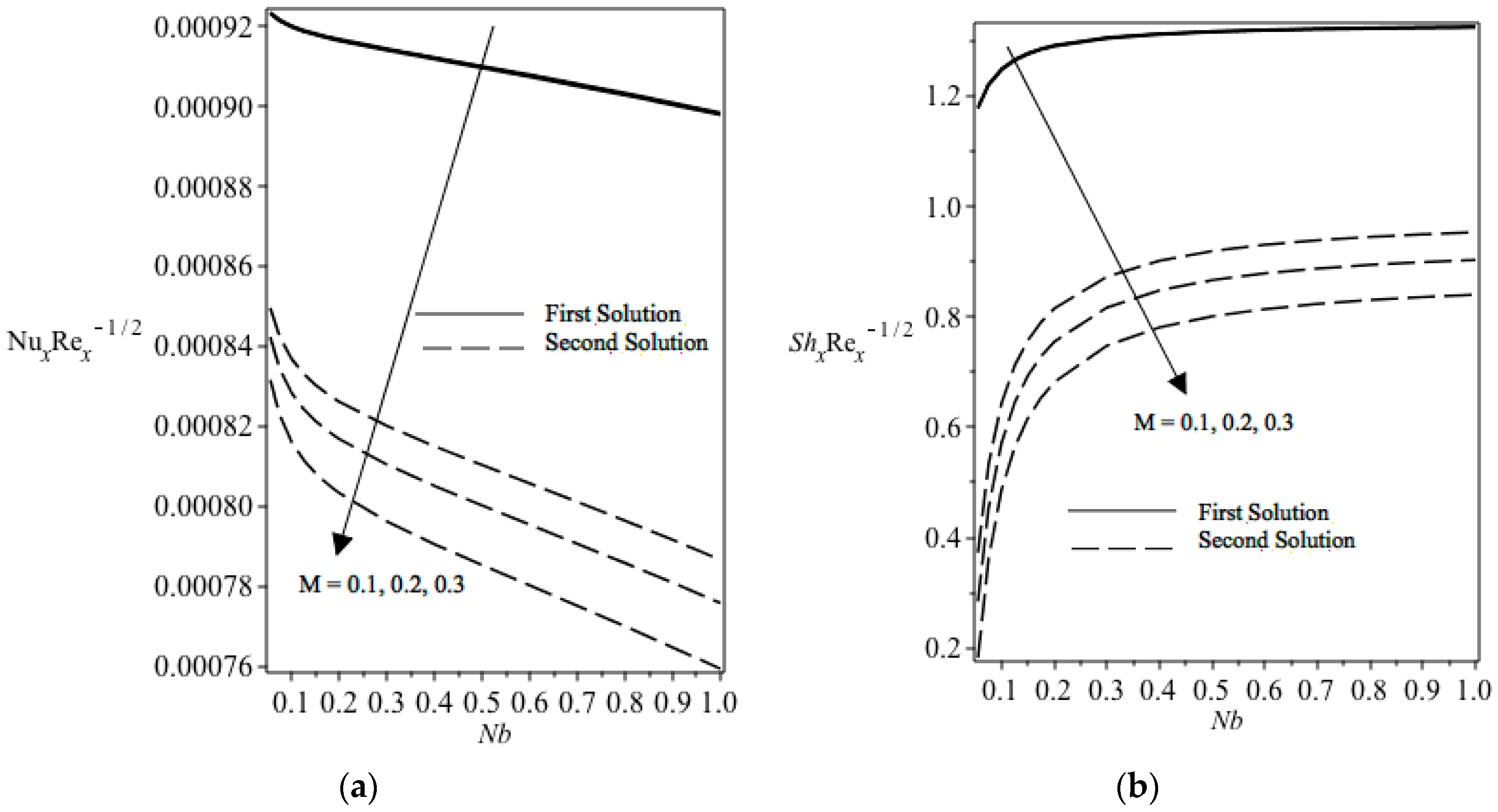
The local Nusselt number and local Sherwood number variations with the parameter of Brownian motion Nb for various influences of the magnetic field parameter M are plotted in Figure 5a,b, respectively, while other parameters are fixed in the stretching case (Pr = 1, Le = 2, Nt = 0.5, Nb = 0.5, Bi = 0.1, $\sigma$ = 0.1, n = 2, Du = 0.2, Sr = 0.1, Ec = 0.1, and S = 2.5). Figure 6a shows that the local Nusselt number values decrease when Nb increases; however, as M increases, the local Nusselt number decreases. Figure 6b shows the local Sherwood number increases when Nb increases but has a lower value when M increases. These graphs illustrate the decreasing trend of the local Nusselt number and local Sherwood number against the Brownian motion parameter as the magnetic parameter increases. This figure also demonstrates that there are nonunique solutions at some level of the magnetic parameter, where the presence of those solutions depends on linear heat and velocity stability. This shows that fluid and thermal motion on the wall of the sheet decelerated when we strengthened the effects of the magnetic parameter.

Based on the results in Figure 2, Figure 3 and Figure 4, the Sh values for Bi, Nt, and Ec against suction are aligned to the Froessling curve in Equation (18). Since Pr = 1, the Sherwood number is calculated with several parameters as stated in Equation (18). The effect of the suction parameter caused the Sherwood number to decrease due to the steeper bubble increase. As the velocities of free bubbles increase, the Reynolds and Schmidt numbers decrease. Based on the results from Figure 5b and Figure 6b, Sh values for Nt and M against Nb are also aligned to the Froessling curve in Equation (18). Since the Sherwood number decreases because of the increasing Brownian motion parameter, the values for Nb, Reynolds number, and Schmidt number also decrease. Since the effect of the suction parameter and Brownian motion parameter decreases the velocities of free bubbles, the Reynolds and Schmidt numbers are smaller due to a larger drag force coefficient.

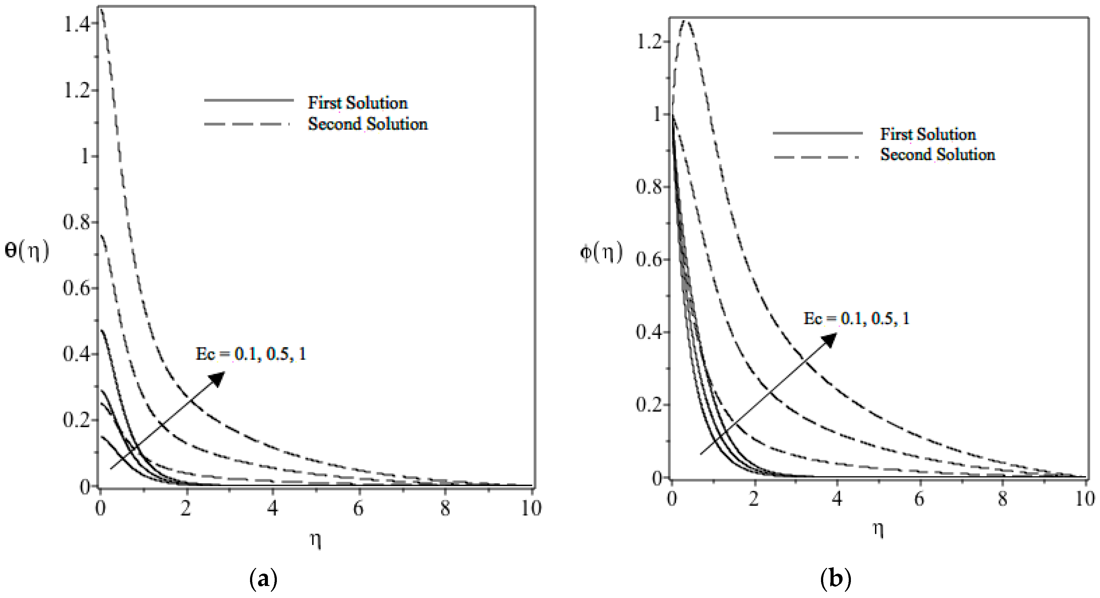
The nanoparticle and temperature concentration profiles for different values of Eckert Ec are respectively shown in Figure 6b and Figure 7a for a stretching surface when all governing parameters are fixed. It is discovered that there are two different profiles for different layer thicknesses with a given mass suction parameter S, which supports the existence of a dual solution, as illustrated in Figure 5a,b. It is found that when Ec increases, the nanoparticle and temperature concentration profiles will decrease and, hence, tend to increase the nanoparticle and thermal boundary layer thicknesses. Figure 7a illustrates the power of the Eckert number Ec on temperature in the boundary layer. By studying the graph, the values of Ec increase when the wall temperature of the sheet increases. This is due to the decrease of heat transfer rate at the surface; thus, the thickness of the thermal boundary layer increases when the value of Ec increases.

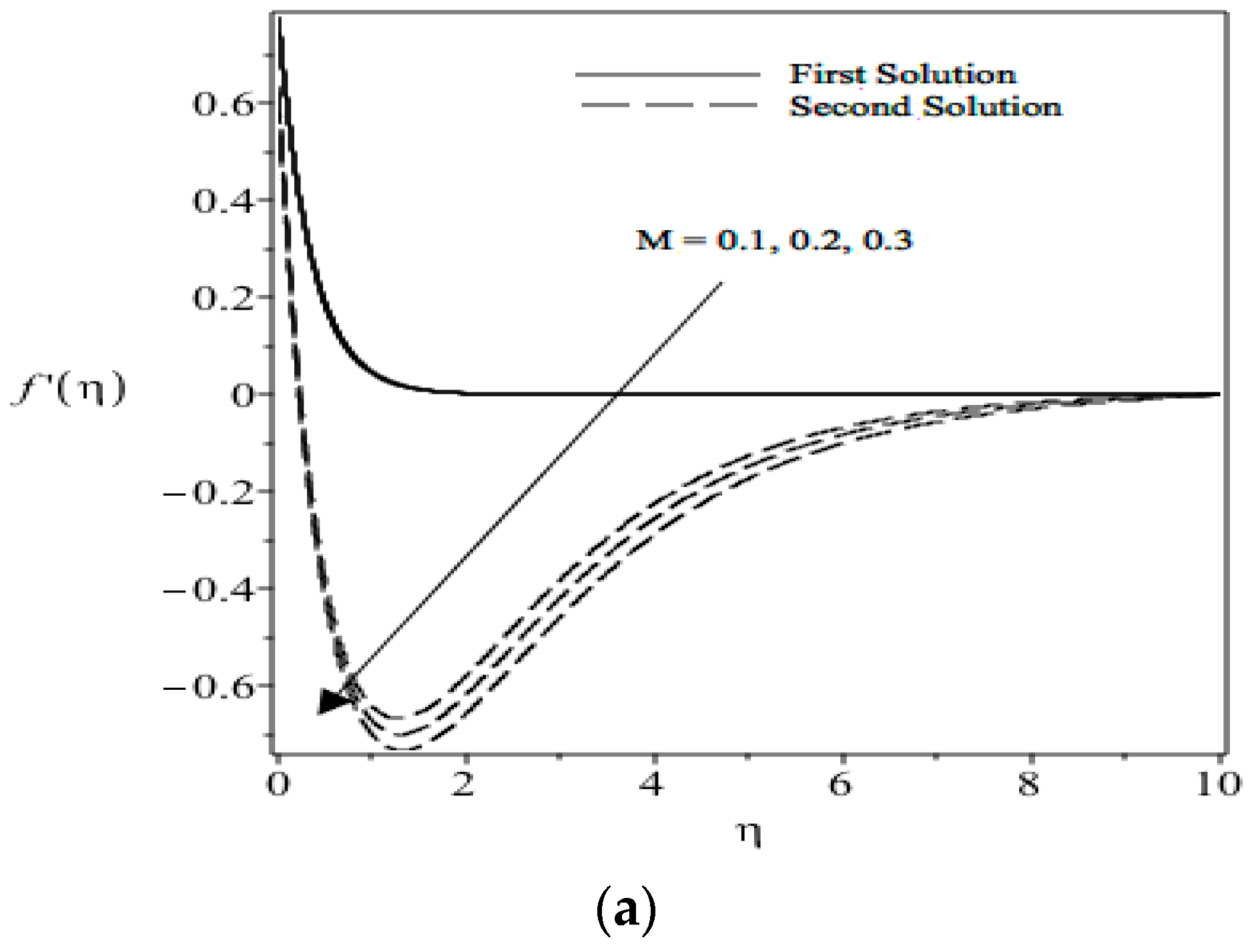
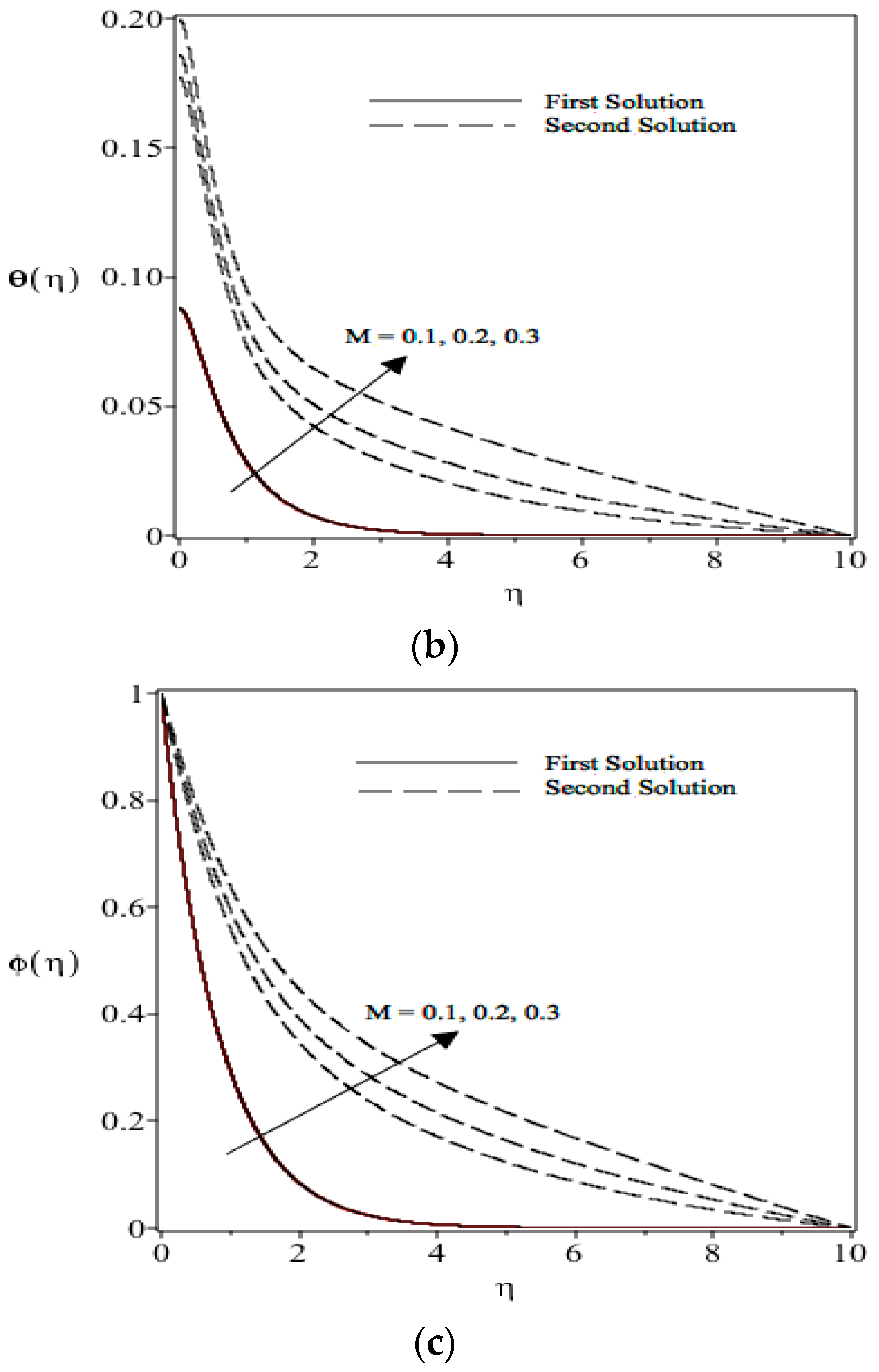
Figure 8a indicates the effect of the magnetic field on the flow field. With the existence of a transverse magnetic field, the fluid induces the Lorentz force, which opposes the flow. This resistive force favors flow deceleration, which results in the decreasing velocity field seen in Figure 6a. We can see that when increasing the value of the magnetic parameter M, the retarding force is also increased along with a reduction in velocity. Figure 8a also shows that when the value of magnetic parameter M increases, the boundary layer thickness is reduced. Figure 8b,c shows that the transverse magnetic field value causes the thermal boundary layer nanoparticle concentration boundary layer to be thicker. This can be explained by the temperature and nanoparticle concentration increment in the boundary layer when the magnetic field is increased.

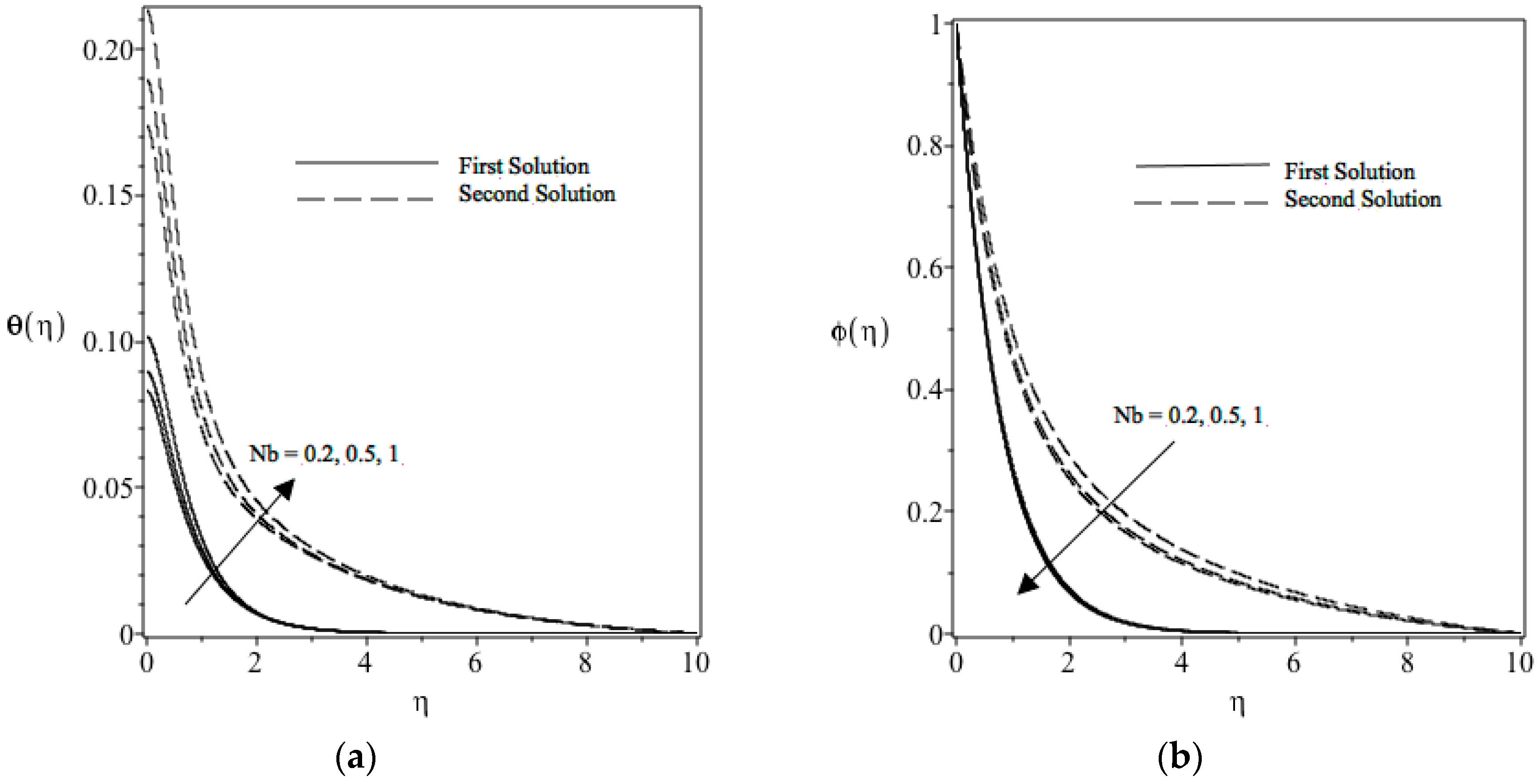
Figure 9a shows the change in the parameter of Brownian motion, Nb, on the temperature profile. Based on our observation, an increase in the Brownian motion parameter leads to temperature increase in the boundary layer. As Brownian motion increases, nanoparticles emigrate from the hot surface towards the cold ambient fluid and, because of that, the temperature will increase in the boundary layer. This will help in thickening the boundary layer. Figure 9b reveals the concentration profile. The concentration profile is a decreasing function of Nb. The reason for this may be that the decrease in the Brownian motion parameter will reduce the mass transfer of a nanofluid.

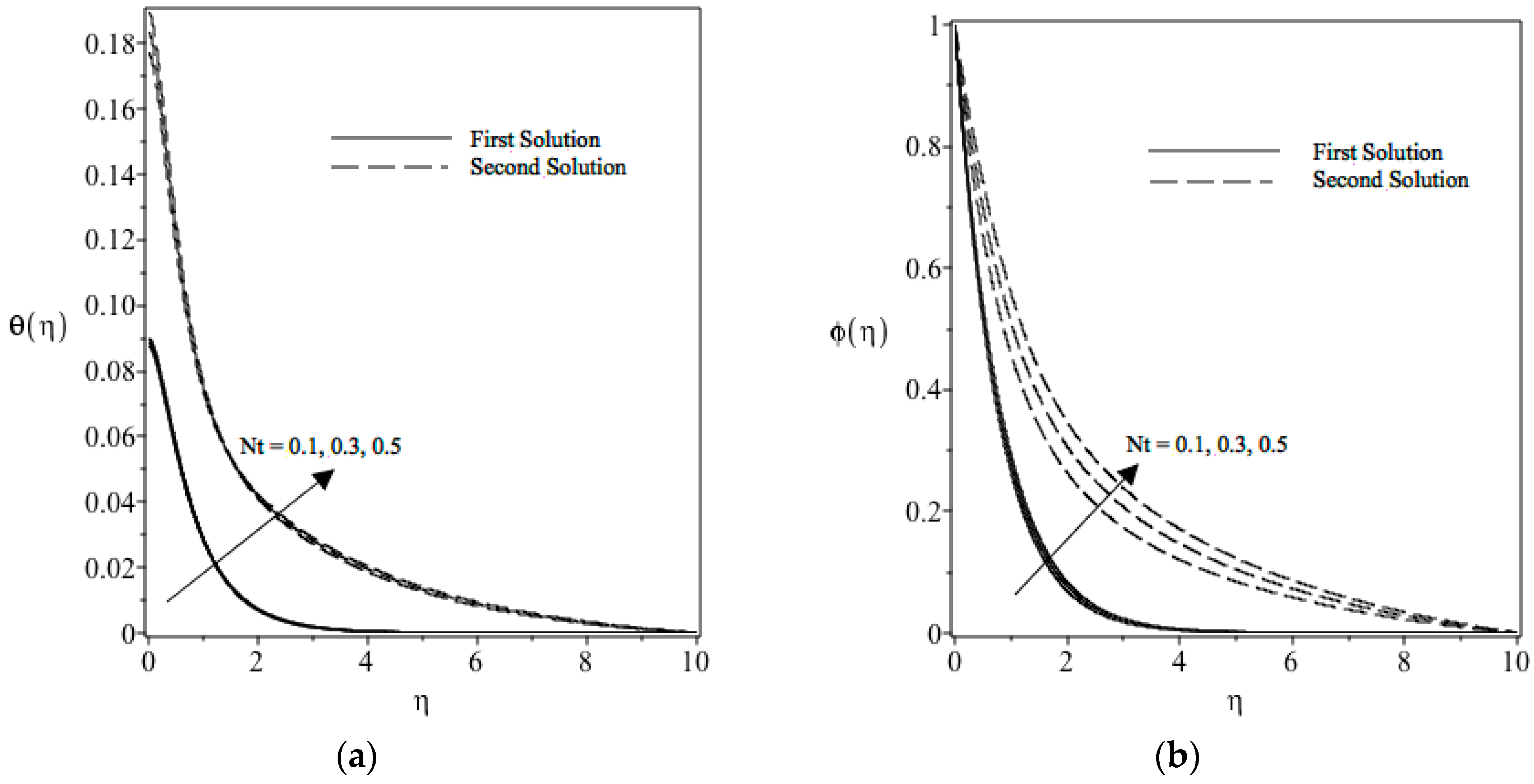
Figure 10a shows the change in the thermophoresis parameter Nt on the temperature profile. When the thermophoresis parameter increases, the temperature increases in the boundary layer. As the thermophoresis effect increases, nanoparticles emigrate from the hot surface towards the cold ambient fluid and, because of that, the temperature will increase in the boundary layer. This will help in thickening the boundary layer. Figure 10b reveals the variation of the concentration profile. The larger values of thermophoresis parameter Nt in 5a lead to larger temperature differences. The concentration field is driven by the temperature gradient. When the temperature is an increasing function of Nt, a rise in the Nt parameters causes the concentration and the boundary layer thickness to increase.

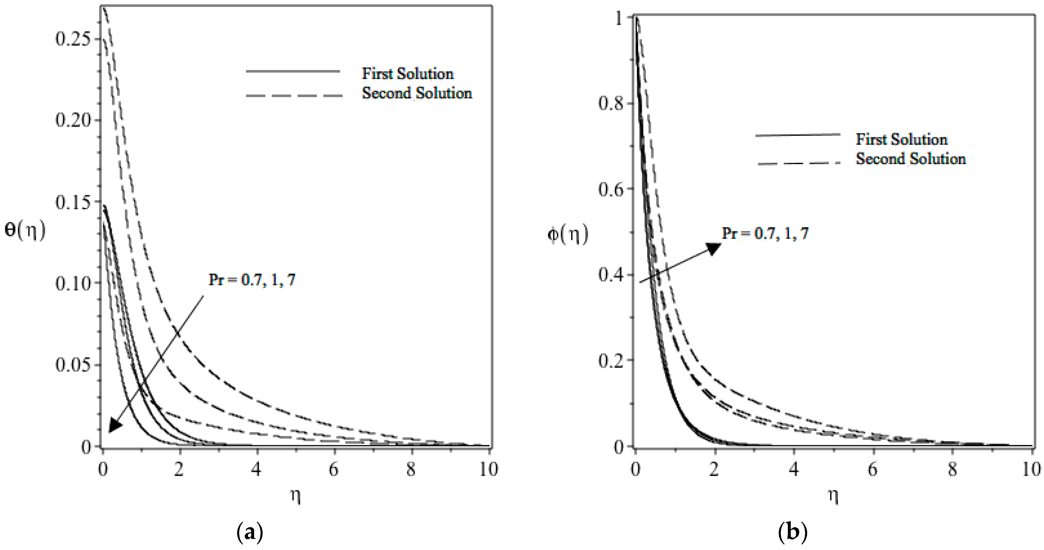
Figure 11a displays the variation of temperature profile with the Prandtl number Pr. The effect of the Prandtl number, Pr, is that an increase in Prandtl number Pr will lead to a decrease the temperature field. Increasing the value of Pr indicates that momentum diffusivity is greater compared to thermal diffusivity. As a result of this, the thermal boundary layer thickness represents a decreasing function of Pr. Figure 11b shows that the momentum diffusivity dominates as the Prandtl number Pr increases. As a result of this, the nanoparticle concentration and boundary layer thickness represent an increasing function of Pr.

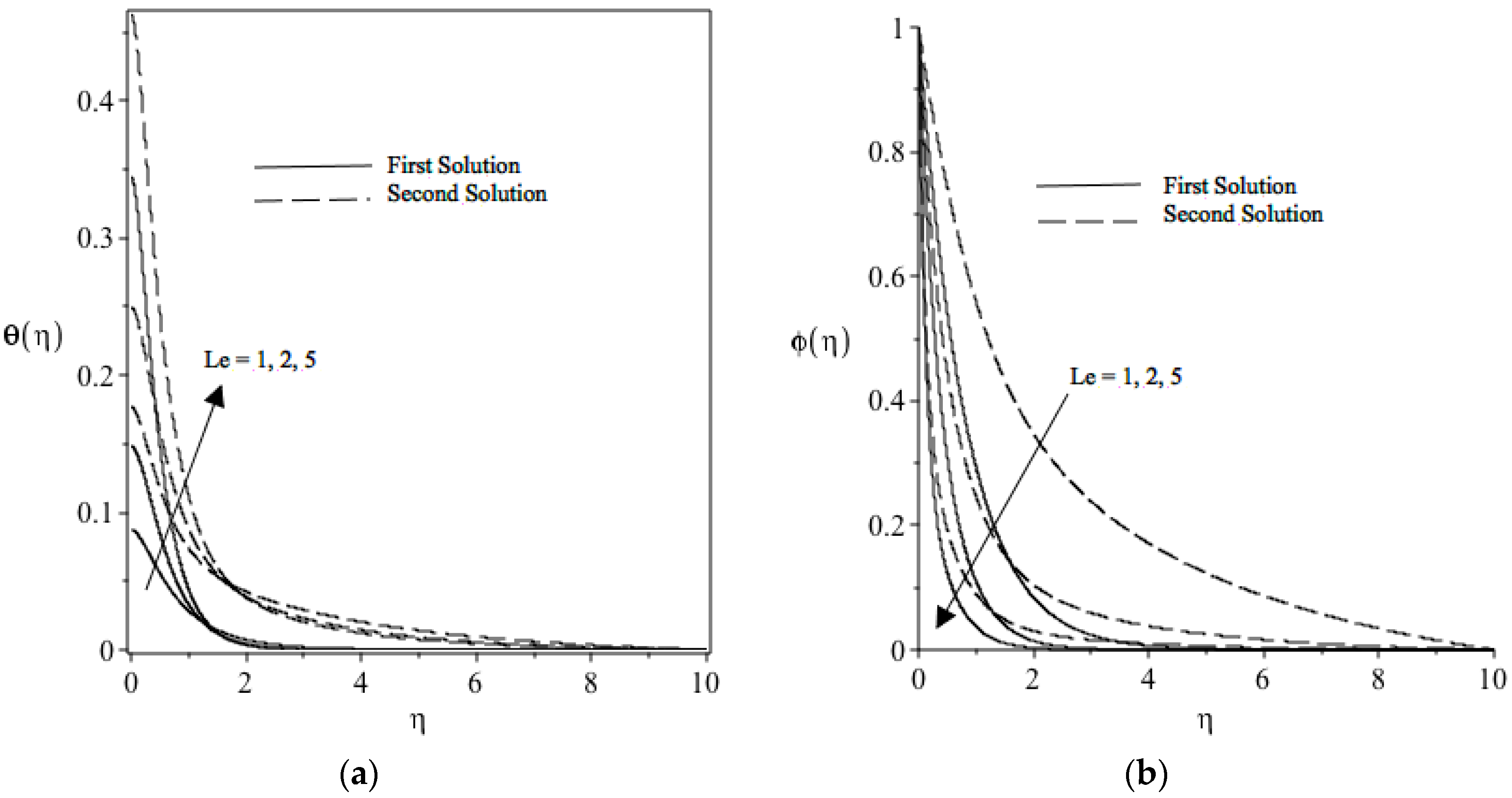
Figure 12a,b respectively show the variation in temperature and nanoparticle concentration when changing the Lewis number Le. A greater value of Lewis number Le indicates higher thermal diffusivity and lower nanoparticle diffusivity. Le > 1 indicates the thermal diffusion rate is above the Brownian diffusion rate. The lower the Brownian diffusion, the lower the mass transfer rate. Results from Figure 12a show that the thermal boundary layer thickness is an increasing function of Le. However, in Figure 12b, we can see that increasing the Lewis number Le results in a thinner nanoparticle concentration boundary layer.

4. Statistical Properties

The influence of magnetic, Eckert, and Biot numbers on the boundary layer flow and heat transfer in a nanofluid over a nonlinearly stretching/shrinking sheet are studied using statistical analysis. To understand what the relationship is between the various physical parameters and also for the local Nusselt number and local Sherwood number, the values of correlation coefficients are calculated. The apparent error of the correlation coefficient can be solved using the formula

P.E (r) = 0.6745 (1 − r²)/sqrt(n),

(19)

where n is the number of observation and r is the correlation coefficient. r > 0.7 indicates a strong linear relationship between parameter variables. If r is less than P.E, the correlation coefficient is not important; this indicates that there is no relationship between variables. The interaction is said to be remarkable when the value of r is 6 times larger than P.E, and insignificant when r is less than P.E(r). The probable error is used to check the accuracy of the value of the correlation coefficient. The values of r/P.E(r) are shown in

Table 3. Values of r/P.E.(r).

	Local Nusselt Number			Local Sherwood Number
	M	Ec	Bi	M	Ec	Bi
r	0.9947	0.9456	0.9509	0.8126	0.9984	0.9988
P.E(r)	0.0018	0.0178	0.0152	0.05914	0.0005	0.0003
r/P.E(r)	543.9791	53.0041	62.5026	13.7404	1973.8055	2731.6587

. From this table, it is obvious that the M, Ec, and and Bi values for heat and mass transfer fulfil the relationship r/P.E(r) > 6, which indicates that the correlation coefficient is statistically significant.

5. Conclusions

The effects of magnetic, Eckert, and Biot numbers on the heat transfer and boundary layer in a nanofluid over a nonlinearly stretching/shrinking sheet are studied in this work. By using similarity transformation, the governing partial differential equations are transformed into ordinary differential equations. Then, by utilizing the shooting method, the problems are solved numerically. The effect of M, Ec, and Bi numbers on velocity, temperature, and nanoparticle concentration profiles as well as the skin friction coefficient, heat, and mass transfer rates are presented graphically. From the obtained numerical results, similar conclusion is found to be the same as [4]. Results from [4] found that an increase in magnetic parameter would decrease the reduced Nusselt and Sherwood number. The same pattern was also found from [6], where M is a decreasing function, and therefore, it enhances the heat transfer.