DA-OCBA: Distributed Asynchronous Optimal Computing Budget Allocation Algorithm of Simulation Optimization Using Cloud Computing

Abstract

The ranking and selection of simulation optimization is a very powerful tool in systems engineering and operations research. Due to the influence of randomness, the algorithms for ranking and selection need high and uncertain amounts of computing power. Recent advances in cloud computing provide an economical and flexible platform to execute these algorithms. Among all ranking and selection algorithms, the optimal computing budget allocation (OCBA) algorithm is one of the most efficient. However, because of the lack of sufficient samples that can be executed in parallel at each stage, some features of the cloud-computing platform, such as parallelism, scalability, flexibility, and symmetry, cannot be fully utilized. To solve these problems, this paper proposes a distributed asynchronous OCBA (DA-OCBA) algorithm. Under the framework of parallel asynchronous simulation, this algorithm takes advantage of every idle docker container to run better designs in advance that are selected by an asymptotic allocation rule. The experiment demonstrated that the efficiency of simulation optimization for DA-OCBA was clearly higher than that for the traditional OCBA on the cloud platform with symmetric architecture. As the number of containers grew, the speedup of DA-OCBA was linearly increasing for simulation optimization.

1. Introduction

The most common goal of simulation studies is the selection of the best system design from a set of competing alternatives. Simulation optimization is a structured approach to determine optimal settings for input parameters (i.e., the best system design) [1], where optimality is measured by a (steady-state or transient) function of output variables associated with a simulation model [2]. Therefore, the study of simulation optimization is particularly crucial. At the same time, due to complexity and randomness (uncertainty factors such as random sampling) of real problems [3], simulation optimization needs to test each design independently many times before it evaluates the results from these designs to select the best [4]. In addition, these real problems may have many parameter combinations that have a large number of simulation designs. These problems lead to increasingly more computing when the problem becomes increasingly complex, so greatly reducing computing is the key to solve the simulation-optimization problem [5]. The ranking and selection method of simulation optimization treats the optimization problem as a multi-index decision problem to select the optimal design from some complex designs that are difficult to represent by mathematical models [6]. Among all ranking and selection algorithms, optimal computing budget allocation (OCBA) [7] is one of the most efficient algorithms for simulation optimization [8]. OCBA uses the method of optimizing computing budget allocation to improve simulation efficiency [9]. The optimization of the simulation budget allocation is done by analyzing the results of the simulation designs periodically to assign the computing budget of the next stage [10]. The objective is to maximize simulation efficiency, expressed as the probability of correct selection (PCS) [11] within a given computing budget. Compared to the traditional two-stage selection procedure [12] for ranking and selection, OCBA is widely used in simulations, and experiments have shown that OCBA is more effective to select the best design under the same PCS [6]. In particular, the current work focuses on improving algorithm efficiency for solving an optimization problem.

Recently, cloud computing, which provides computational powers on demand via a symmetric network, has gained a lot of popularity among users who need to flexibly handle surges of demand for computing power [13]. The network allows all devices to send and receive data at the same rate and is named symmetric network. Symmetric networks support more bandwidth in one direction as compared to the other, and symmetric architecture offers clients the same bandwidth for both downloads and uploads. Therefore, symmetric architecture ensures that all computers on the symmetric network have equal opportunities to discover, publish, and receive content. Symmetric network design gives all devices equal access to resources. Symmetric computing means the equal sharing of resource access between different users in the cloud. Cloud computing provides new ideas for simulation optimization. First, when using cloud-computing resources, users only need to pay for the service without owning software or hardware, which leads to lower costs of centralized deployment of software or hardware for high performance [14]. Second, it is easier to scale computing power in a cloud platform with symmetric architecture than in a high-performance computer cluster [13]. The scale of symmetric computing resources can flexibly meet the needs of users. For instance, if users have a sudden surge demand in computing resources on the computing platform, then they only need to pay the related computing resources of the cloud platform. Users do not need to install additional devices. Cloud computing not only reduces high costs but also provides flexible high-performance computing to meet the needs of simulation optimization for elastic computing [15]. Therefore, the cloud-computing platform has good prospects for solving the simulation-optimization problem. However, OCBA only runs a small number of simulation designs step by step, and each step deletes simulation designs to be run in the next step, based on experimental data from all previous simulation designs [9]. Due to this principle, each step is short of a sufficient number of designs that can be parallel-run in each step of a simulation-optimization process. Despite the scale of computing being reduced, there is a certain delay during simulation optimization because of serial features between the different steps. As a result, the performance advantages of the cloud-computing platform cannot be fully utilized. Therefore, it is important to take advantage of the flexibility, scalability, symmetry, and parallelism of the cloud-computing platform on the basis of the lower scale of simulation optimization.

To solve these problems, this paper proposes the distributed asynchronous OCBA (DA-OCBA) algorithm. This algorithm pre-executes all designs several times. Then, DA-OCBA uses the idle docker containers at present to run better designs in advance that are selected by an asymptotic allocation rule, so DA-OCBA can efficiently select the optimal designs in any computing resource. At the same time, the results for all designs of every step are stored. If the current designs have been executed extra times, we just directly use these results without running it again. DA-OCBA loops, in turn, until it reaches the computing budget or the PCS. During the execution of this algorithm, we set up a uniform sequence of random numbers to ensure serial and parallel result accuracy. This algorithm makes full use of the parallelism, flexibility, and scalability of cloud computing. We achieved asynchronous operation of the algorithm for the execution and selection of designs by running designs in advance. During the execution of this algorithm, the designs were constantly run. Finally, the results further indicated that the simulation-optimization efficiency for DA-OCBA is clearly higher than that of OCBA. At the same time, the remaining idle containers were used to run better designs that would have been selected by an asymptotic allocation rule. The asymptotic-allocation rule guarantees that DA-OCBA uses a similar total computing budget compared to OCBA.

The rest of this paper is organized as follows: Section 2 describes background and related works. Section 3 introduces our problem analysis. Section 4 explains the proposed system architecture and DA-OCBA framework. Section 5 presents the experimental case and environment. Section 6 outlines the experiment results and performance discussion. Section 7 concludes the paper.

2. Background and Related Works

2.1. Simulation Optimization, Ranking, and Selection

Simulation optimization can be used to cope with uncertainties since it allows us to model and evaluate the uncertainties in the system. Simulation optimization plays a central role in the design and efficient management of complex human-made systems such as communication and transportation systems and manufacturing facilities, as closed-form analytical solutions are difficult to solve. There are some methods of simulation optimization including metamodeling, sample average approximation, and gradient-based method. However, when certain decision variables are discrete and the structure of the problem is unknown, these methods may not be applicable. Another option is to use derivative-free, black-box simulation. When the number of alternatives to be selected is fixed, the problem comes down to a statistical selection problem called ranking and selection [16].

The ranking and selection program is a specially developed statistical method for selecting the best design or a subset of the best designs from a set of k competing design alternatives [17]. So many rankings and selection methods have emerged such as two-stage procedures by Dudewicz and Dalal [18] and Rinott [19], the two-stage procedure with screening by Nelson et al. [20], or the fully sequential procedure by Kim and Nelson [21]. In their procedures, if the difference is greater than the specified parameter or if the decision maker is indifferent, the difference is considered important. Therefore, they are called indifference zone (IZ) procedures. Another popular approach is to maximize the probability of correct selection (PCS) given a computing budget called Optimal Computing Budget Allocation (OCBA).

Table 1. Key differences between Optimal Computing Budget Allocation (OCBA) and indifference zone (IZ).

Comparison	OCBA	IZ
Focus	Efficiency (maximizing probability of correct selection (PCS))	Feasibility (finding a feasible way to guarantee PCS)
Total number of simulation samples	Equal to the computing budget which is set by the user	Uncertain (it depends on when the stopping rule is set to guarantee PCS)
PCS	The actual PCS is unknown. However, PCS can also be guaranteed as long as the value of Approximate PCS (APCS) is greater than the expected PCS. (Note that APCS is easy to calculate as shown in Section 3.2.)	The expected PCS is guaranteed to be achieved. The actual PCS is unknown and it is usually much higher than the expected PCS because the procedure is developed based on the most unfavorable configuration.
Assumptions	Based on Bayesian and Frequentist view	Based on Frequentist view

provides the key differences between the OCBA and IZ approaches [16].

By analyzing the least favorable configuration, ranking and selection can guarantee a predetermined lower bound on the PCS [22,23,24]. The downside of the ranking and selection framework is that it usually allocates more replications than is necessary to guarantee the PCS.

Alternatively, the optimal sampling allocation framework maximizes PCS by a limited simulation budget, which typically results in a higher PCS with a specified simulation budget, or uses less simulation to achieve the same level of PCS. As simulation, which is time consuming, is used to estimate the performance measure, efficiency becomes a key issue. Highlighted in this framework is the OCBA method with its mean and variance trade-off properties [25]. OCBA focuses on the efficiency issue by intelligently controlling the number of simulation replications based on the mean and variance information. Intuitively, to ensure a high probability of correctly selecting the desired optimal designs, a larger portion of the computing budget should be allocated to those designs that are critical in identifying the necessary ordinal relationships. In order to obtain a closed-form solution for the ratio (weight) of the number of replications assigned to each design, OCBA assumes that the parameters of the underlying design are known and relaxes the objective function with Bonferroni’s inequality. In practice, sample statistics are used to obtain an initial estimate of the first-stage parameters based on a small portion of the simulated budget and use the parameter estimates that are in the OCBA formula to allocate the remaining replications. Although the resulting OCBA algorithm is heuristic, it has been successfully applied to heuristic algorithms, which have been successfully applied to many practical problems [26,27]. The OCBA solution can also be used as an approximate solution to the optimization problem defined by the exponential rate of the large deviation probability that maximizes the wrong choice [28,29]. OCBA was also studied in the Bayesian framework [30], but the formula for parameter-optimization problems did not consider order assignment. However, Chen et al. [31] showed that the performance of the OCBA algorithm under perfect information (assuming the parameters are known) may be much lower than the performance of the sequential OCBA algorithm.

Chen et al. [10] found that the OCBA algorithm is an ideal method for solving stochastic-simulation-optimization problems. The integration of the modified OCBA algorithm and the appropriate search algorithm becomes a complete process of simulation optimization. This method was originally applied to solve the unconstrained single-objective simulation-optimization problem. Compared with the traditional two-stage method, this method not only is efficient but also has good robustness. Branke et al. [32] also pointed out that the OCBA algorithm is one of the most efficient algorithms among the existing statistical methods through a large number of numerical experiments. Later, Chen et al. [9] extended it to the single-objective simulation-optimization problem for selecting the optimal subset. In this subset, the designs were no longer sorted. Lee et al. considered the case with constraints; they applied it to the single-objective simulation-optimization problem with random constraints through the improved OCBA algorithm, and they gave a simulation-calculation allocation rule with a constraint condition.

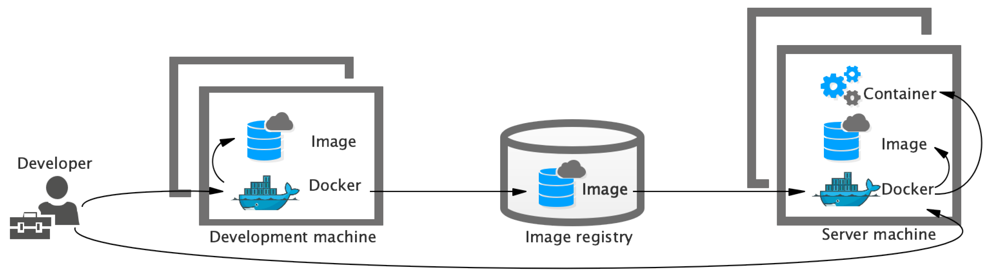
2.2. Cloud Computing with Ranking and Selection

The distributed computing system represented by cloud computing provides new ideas for simulation optimization. In the meantime, the high performance, flexibility, scalability, and parallelism of cloud computing [33] have good prospects for applying cloud computing to simulation optimization. Now that cloud computing is becoming more available, we ask if the existing ranking and selection procedure is suitable for cloud frameworks. To solve this question, Kim and Nelson (KN) [34] summarized the sequential nature of simulations on a single processor, that is, sequentially generating data on a single processor. Cloud computing provides us with a large number of docker containers that can work in parallel, and the ordering of each container still applies. Therefore, we used a master/slave structure to design a program that allows a container to process a design and to run all designs in parallel. Another feature of cloud computing is the asynchronousness between different containers that leads to various design sizes for different systems. Asynchrony may be due to different configurations of their containers or delayed/lost packets due to network environment or transport protocols. Then, most existing algorithms, such as the KN process, require the same design size and are not suitable for cloud frameworks. As far as we know, there are only two ranking and selection simulation-optimization algorithms for cloud computing [35,36]. However, at the same time, the need for smaller computing budgets and higher computational efficiency cannot be met. In fact, these ranking and selection algorithms run on a high-performance computing platform rather than the actual cloud. Too little work is devoted to applying ranking and selection to cloud platforms. Therefore, it is necessary to create a ranking and selection algorithm so that we can take full advantage of cloud computing.

2.3. Simulation Analytics and Random Number

A simulation analysis is more than just “saving all simulation data” but also applies modern data-analysis tools (although this capability is beneficial in itself) [37]. Instead, simulation–analysis studies should address and exploit the differences between simulated data and real-world transaction data as well as differences in the context of the problem that needs to be simulated rather than on-site data analysis. Some of the features that distinguish a simulated-analysis context from a big data analysis context are as follows:

• Simulation data are clean, complete, and can easily be organized (but should not be summarized) and generated. In addition, within the computation of budget constraints, the amount of data is under our control.
• Probability models that describe the underlying stochastic inputs are known and are also under our control, as are the random-number assignments that generate realizations [38].
• Logical structures that cause state transitions (e.g., entity networks or agent rules) are also known and can be manipulated.

As was mentioned above, it is important for us to keep a uniform sequence of random numbers between serial and parallel. Only in this way can we obtain correct results from simulation optimization.

3. Problem Statement

In this section, we introduce the principle for DA-OCBA, such as symbol description, the definition of a discrete event system (DES), PCS, and the asymptotic allocation rule.

3.1. Discrete Event System

The general simulation and optimization problem of this DES can be defined as follows:

$$mi{n}_{\theta \in \mathsf{\Theta }}\overline{J}({\theta }_i)\equiv E[L(\theta ,\omega )]$$

(1)

The standard approach is to estimate $E[L(\theta ,\omega )]$ by the sample mean performance measure:

$${\overline{J}}_i\equiv \frac{1}{N_i}\sum _{j=1}^{k}L({\theta }_i,{\omega }_{ij})$$

(2)

where ${\omega }_{ij}$ represents the jth sample of $\omega$ and $N_i$ represents the number of simulated samples designed for i.

As $N_i$ increases, ${\overline{J}}_i$ becomes closer to $J({\theta }_i)$ because its corresponding confidence interval becomes narrower. The final accuracy of this estimate cannot be improved faster than $1/\sqrt{N}$. Note that each sample of $L({\theta }_i,{\omega }_{ij})$ requires a simulation run. The large number of $L({\theta }_i,{\omega }_{ij})$ samples required for all designs can become very time consuming.

3.2. Probability of Correct Selection

We focus on the selection of the smallest k designs, which is not uncommon, as the proposed method is equally applicable to the selection of the largest design. Although a design with a minimum sample mean (design b) is typically selected, design b is not necessarily the design with the least unknown mean performance. Therefore, CS is defined as that since design b is actually the best design. We want to maximize the probability of correctly identifying the true best design, PCS, for a given computing budget T. Assume that the computational cost of each copy is roughly the same in different designs. Then, computational cost can be approximated as $N_1+N_2+\dots +N_k$, which is the total number of replications. For some stochastic systems, the computational cost of simulating different designs is not the same. Our approach can easily be modified to include such cases. Ideally, we want

$$\begin{array}{c}\begin{array}{c}{max}_{N_1,\dots ,N_k}PCS\hfill \\ s.t.N_1+N_2+\dots +N_k=T.\hfill \end{array}\hfill \end{array}$$

(3)

If we select the observed best design, the probability that we selected the best design is

$$\begin{array}{cc}\hfill PCS& =P\{bisthebest\}\hfill \\ & \hfill =P\{J({\theta }_b)<J({\theta }_i),i\ne b|L({\theta }_i,{\omega }_{ij})\},j=1,\dots ,N_i,i=1,2,\dots ,k\}\end{array}$$

(4)

To simplify the symbols used, we rewrote Equation (4) as $P\{{\tilde{J}}_b<{\tilde{J}}_i,i\ne b\}$, where ${\tilde{J}}_i$ denotes a random variable in which the probability distribution is the posterior distribution of design i. Assume that unknown mean $J({\theta }_i)$ has a conjugate normal a priori distribution. We consider the previous distribution without information. This means that no prior knowledge is given about the performance of any design alternative before conducting the simulation. In this case, DeGroot indicates that the posterior distribution of $J({\theta }_i)$ is

$$\widetilde{J_i}\sim N(\overline{J_i},\frac{s_i^2}{N_i})$$

(5)

After the simulation is performed, ${\overline{J}}_i$ can calculated and $s_i^2$ can be approximated by the sample variance. Then, the Monte Carlo simulation can be used to estimate PCS. However, estimating PCS by Monte Carlo simulation is time consuming. Since the purpose of budget allocation is to improve simulation efficiency, we need a relatively fast and inexpensive way to estimate PCS within the budget-allocation procedure. In this case, efficiency is more important than estimation accuracy. We use a general approximation procedure used in the simulation and statistical literature [39]. This approximation is based on the Bonferroni inequality.

$$\begin{array}{c}\hfill \begin{array}{cc}\hfill PCS& =P\{\bigcap _{i=1,i\ne b}^k(\widetilde{J_b}-\widetilde{J_i}<0)\}\hfill \\ & \ge 1-\sum _{i=1,i\ne b}^k[1-P\{\widetilde{J_b}-\widetilde{J_i}<0\}]\hfill \\ & \hfill =1-\sum _{i=1,i\ne b}^{k}P\{\widetilde{J_b}>\widetilde{J_i}\}=APCS\end{array}\end{array}$$

(6)

We refer to this lower bound of the correct selection probability as the approximate PCS (APCS) [40]. APCS can be calculated very easily and quickly; no additional Monte Carlo simulation is required. Numerical experiments have shown that APCS approximation can still lead to efficient procedures [41,42]. Therefore, as the simulation experiment progressed, we used APCS to approximate PCS. More specifically, we consider the following questions:

$$\begin{array}{c}{max}_{N_1,\dots ,N_k}PCS\simeq ma{x}_{N_1,\dots ,N_k}1-\sum _{i=1,i\ne b}^{k}P\{\widetilde{J_b}>\widetilde{J_i}\}\hfill \\ s.t.\sum _{i=1}^k{N}_i=Tand{N}_i\ge 0.\hfill \end{array}$$

(7)

Then, we introduced an asymptotic-allocation rule with respect to the number of simulation replications; $N_i$ is presented.

3.3. The Asymptotic Allocation Rule

As is shown in Equation (7), we can get the objective function, ${\delta }_{b,i}={\overline{J}}_b-{\overline{J}}_i$, and ${\overline{J}}_b\le {\overline{J}}_i$.

$$\begin{array}{cc}\hfill \sum _{i=1,i\ne b}^{k}P\{\widetilde{J_b}>\widetilde{J_i}\}& =\sum _{i=1,i\ne b}^k{\int }_0^{\infty }{\frac{1}{\sqrt{2\pi }{s}_{b,i}}}^{\frac{{(x-{\delta }_{b,i})}^2}{2s_{b,i}^2}}dx\hfill \\ & =\sum _{i=1,i\ne b}^k{\int }_{-\frac{{\delta }_{b,i}}{s_{b,i}}}^{\infty }\frac{1}{\sqrt{2\pi }}{e}^{\frac{t^2}{2}}dt\hfill \end{array}$$

(8)

This objective function is based on standard normal probability density function, its properties are as follows:

• Concentration: The peak of the normal curve is in the center, where the mean is located.
• Symmetry: The center of the normal curve is the mean, the normal curve is left–right symmetric, and the ends of the curve never intersect the horizontal axis.
• Uniform variability: The normal curve starts from the place where the mean is located, and the curve gradually decreases uniformly toward the left and right sides.

In the meantime, the standard normal cumulative distribution function is shown in Equation (9); its properties are as follows:

$$\mathsf{\Phi }(x)={\int }_{-\infty }^x\frac{1}{\sqrt{2\pi }}{e}^{\frac{t^2}{2}}dt$$

(9)

• The normal cumulative distribution function is an X-axis monotonically increasing function.
• The normal cumulative distribution function is normalized; this function is monotonically increasing, and it approaches 1.

When two designs are compared, say, designs b and i, we have the following:

$$\begin{array}{c}\hfill \begin{array}{cc}\hfill \widetilde{J_b}-\widetilde{J_i}& \sim N\left({\overline{J}}_b-{\overline{J}}_i,\frac{s_b^2}{N_b}+\frac{s_i^2}{N_i}\right)\hfill \\ \hfill P\{\widetilde{J_b}>\widetilde{J_i}\}& =P\{\widetilde{J_b}-\widetilde{J_i}>0\}=\mathsf{\Phi }\left(\frac{{\overline{J}}_b-{\overline{J}}_i}{\sqrt{\frac{s_b^2}{N_b}+\frac{s_i^2}{N_i}}}\right)\hfill \end{array}\end{array}$$

(10)

According to the standard normal cumulative distribution function, we succeeded in obtaining PCS. Chen et al. [9] showed that the APCS can be asymptotically maximized:

Theorem 1.

Given the total number of simulation samples T to be assigned to k competing designs, the performance is described by random variables, including $J({\theta }_1),J({\theta }_2),\dots ,J({\theta }_k)$ and finite difference $s_1^2,s_2^2,\dots ,s_k^2$, respectively, $T\to \infty$, where $N_i$ is the number of samples assigned to design i [25].

$$\frac{N_i}{N_j}={\left(\begin{array}{c}\frac{s_i/{\delta }_{b,i}}{s_j/{\delta }_{b,j}}\end{array}\right)}^2,i,j\in 1,2,\dots ,k,i\ne j\ne b$$

(11)

$$N_b=s_b\sqrt{\sum _{i=1,i\ne b}^k\frac{N_i^2}{s_i^2}}$$

(12)

In the case of $k=2$ and $b=1$, Theorem 1 returns the following:

$$N_1=s_1\sqrt{\frac{N_2^2}{s_2^2}}$$

(13)

Therefore,

$$\frac{N_1}{N_2}=\frac{s_1}{s_2}$$

(14)

The evaluation results are the same as the well-known best allocation solution for $k=2$.

To gain better insight into this approach, consider another situation where $k=3$ and $b=1$, which yields

$$\frac{N_2}{N_3}=\frac{s_2^2{\delta }_{1,3}^2}{s_3^2{\delta }_{1,2}^2}$$

(15)

We can see how the number of simulated samples of Design 2, $N_2$, is affected by different factors. For the minimization problem, when ${\overline{J}}_3$ increases (we have more confidence in the difference between Design 1 and Design 3) or when $s_2$ increases (we are not sure about Design 2), $N_2$ also increases. On the other hand, when ${\overline{J}}_2$ increases (we have more confidence in the difference between Designs 1 and 2) or when $s_3$ increases (we are not sure about Design 3), $N_2$ decreases. The above relationship between $N_2$ and other factors is consistent with our intuition. Theorem 1 is shown in Algorithm 1.

To address the problem of using OCBA in a cloud platform with Theorem 1, we present cost-effective sequential parallel approach DA-OCBA to select the best design from k alternatives with a given computing budget or PCS in Section 4.

Algorithm 1 Theorem 1—Obtain the number of simulation samples for every competing design.

Input: mean of designs ${\overline{J}}_i$, variance of designs ${\sigma }_i$, one-step budget for simulation $\mathsf{\Delta }$, total number of designs k, number of every design running $SU{M}_i$, number of every design running in the next $N_i$, best design b, second-best design s, $0\le i<k$ Output: number of designs used to run $N_i$  1: $ratio\left[k\right],temp=0,sum=0$;  2: for$i\leftarrow 0,k-1$do  3: $sum=sum+SU{M}_i$;  4: end for  5: $sum=sum+\mathsf{\Delta }$,$su{m}_0=sum$;  6: for$i\leftarrow 0,k-1$do  7:    if $i\ne b$ && $i\ne s$ then  8: $temp=({\overline{J}}_b-{\overline{J}}_s)/({\overline{J}}_b-{\overline{J}}_i)$;  9: $ratio\left[i\right]=temp\ast temp\ast {\sigma }_i/{\sigma }_s$; 10:    end if 11: end for 12: $ratio\left[s\right]=1.0$; 13: $temp=0$; 14: for$i\leftarrow 0,k-1$do 15: $morerun\left[i\right]=1$; 16:    if $i\ne b$ then 17: $temp=temp+(ratio\left[i\right]\ast ratio\left[i\right]/{\sigma }_i)$; 18: $ratio\left[i\right]=temp\ast temp\ast {\sigma }_i/{\sigma }_s$; 19:    end if 20: end for 21: $ratio\left[b\right]=\sqrt{{\sigma }_b\ast temp}$; 22: $more\_alloc=1$; 23: while$more\_alloc$do 24: $more\_alloc=0$; 25: $ratio\_s=0.0$; 26:    for $i\leftarrow 0,k-1$ do 27:     if $morerun\left[i\right]$ then 28: $ratio\_s=ratio\_s+ratio\left[i\right]$; 29:     end if 30:    end for 31:    for $i\leftarrow 0,k-1$ do 32:     if $morerun\left[i\right]$ then 33: $N_i=\lfloor (su{m}_0/ratio\_s\ast ratio\left[i\right])\rfloor$; 34:      if $N_i<SU{M}_i$ then 35: $N_i=SU{M}_i$; 36: $morerun\left[i\right]=0$; 37: $more\_alloc=1$; 38:      end if 39:     end if 40:    end for 41:    if $more\_alloc$ then 42: $su{m}_0=sum$; 43:     for $i\leftarrow 0,k$ do 44:      if $!morerun\left[i\right]$ then 45: $su{m}_0=su{m}_0-N_i$; 46:      end if 47:     end for 48:    end if 49: end while 50: $su{m}_0=N_0$; 51: for$i\leftarrow 1,k-1$do 52: $su{m}_0=su{m}_0+N_i$; 53: end for 54: $N_b=N_b+sum-su{m}_0$; 55: for$i\leftarrow 1,k-1$do 56: $N_i=N_i-SU{M}_i$; 57: end for

4. System Architecture and the DA-OCBA Framework

This section presents the framework of DA-OCBA and some theories of DA-OCBA.

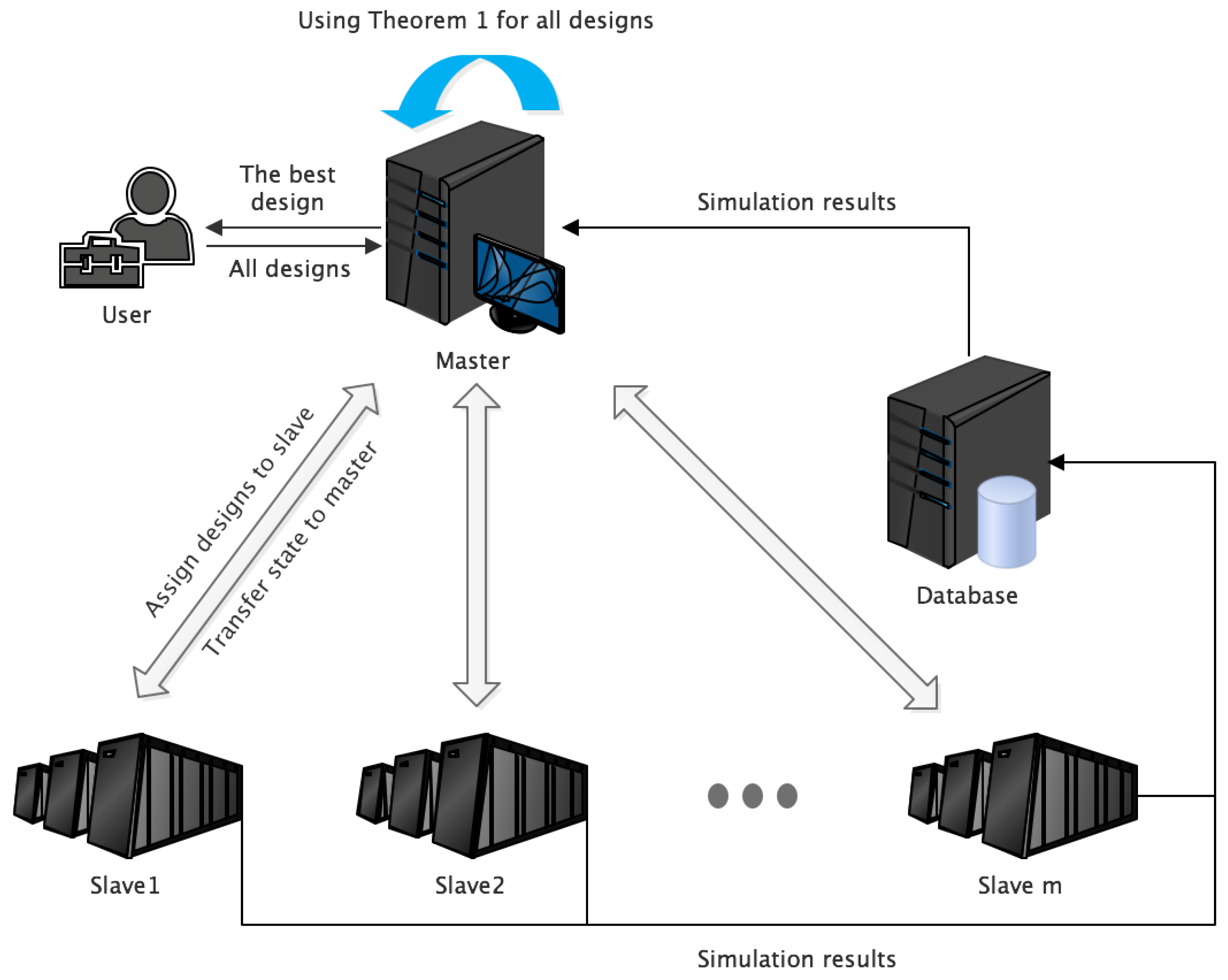
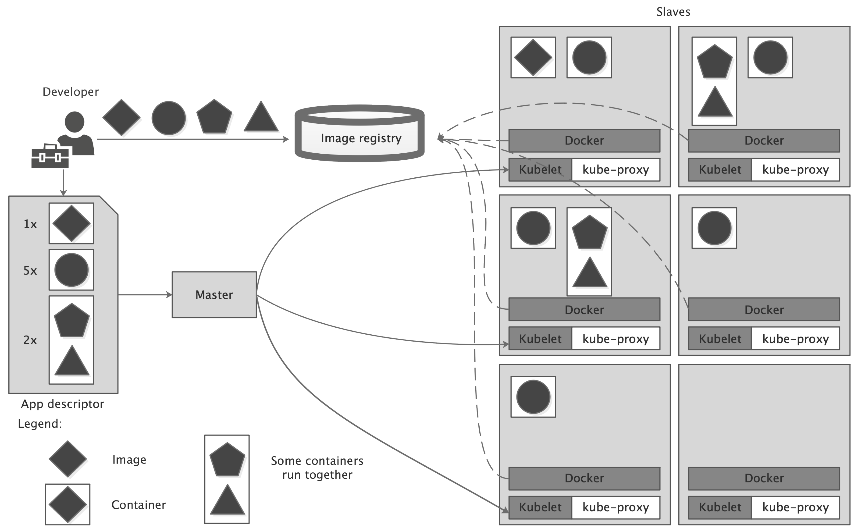
4.1. Architecture for Cloud Platform

At present, large, monolithic applications are being broken down into small standalone components named microservices that are composed of a single process. It is well known to us that the docker container is seen as a sandbox. Everyone runs an application, they are isolated from each other, and communication mechanisms can be established between them. The creation and stopping of the containers are very fast, and it has very limited resource requirements, far below a virtual machine. A process running in a container actually runs on the operating system of the host, which is different from the procedure of a virtual machine running on a different operating system. Therefore, we used containers as the computing unit of the cloud-computing platform with symmetric architecture to take full advantage of hardware resources. The running mechanism of the docker is as follows in Figure 1.

Developers use dockers to produce images in development machines. Then, the development machines upload images to an image repository, from which server machines download the image. Meanwhile, developers assign tasks to the docker in the server machines.

There are a large number of docker containers that need to be managed by an efficient interactive mechanism. Kubernetes is such an open-source application for managing containerized applications on multiple hosts in a cloud platform. The goal of Kubernetes is to make containerized applications to be efficiently deployed. Kubernetes is based on the distributed cloud platform, as shown in Figure 2, and the detailed framework of Kubernetes is shown in Figure 3.

As is shown in Figure 2 and Figure 3, we used Kubernetes to manage docker containers that run designs in a distributed cloud platform with symmetric architecture [43]. Kubernetes follows the master–slave architecture, where a master provides centralized control for all docker containers of slaves. The developer inputs all simulation-optimization designs to the master, and  Kubernetes evenly assigns all designs to the work nodes (slaves), which store the results to the database. According  to the computing budget of the present step, the master obtains the results from the database to assign designs in the next step.

4.2. DA-OCBA Framework

To solve the ranking and selection problem of cloud computing, we propose the DA-OCBA algorithm to take full advantage of cloud-computing resources at each stage that run some design in advance by the idle containers. However, the OCBA does not do this in advance, as shown in Steps 3 and 4. In summary, we have the following DA-OCBA algorithm (assuming $T-k\ast n_0$ is a multiple of $\mathsf{\Delta }$).

Step 1: Input the design initial value, number of designs k, and computing budget T or the probability of correct selection $PC{S}_0$, initial number of simulations $n_0$, number of docker containers $ND$, and computing budget $\mathsf{\Delta }$ at each stage ($m\ast \mathsf{\Delta }=T-k\ast n_0$, m is a natural number, and $\mathsf{\Delta }<ND$).

Step 2: Let $l=0$; each design is initially run for $n_0$ times that uses all docker containers, and the result of each design is stored in the database. The initial number of executions is $N_i^l=n_0$, optimal design b is selected so that the mean is the smallest, and PCS is obtained according to Algorithm 2 to determine whether $PC{S}_0$ is satisfied and to output the optimal design; otherwise, the DA-OCBA continues.

Step 3:$l=0$, according to the mean and variance of all designs, theoretical number $N_i^l$ of each step is obtained to run by Theorem 1 so that their sum is equal to $\mathsf{\Delta }<ND$. Due to $\mathsf{\Delta }<ND$, there are $ND-\mathsf{\Delta }$ docker containers that are free. We use these idle containers to run the designs under the rate of $\mathsf{\Delta }$ at present; their results are stored in the database.

Step 4:$l=1$ at the next step if some ($n^{\prime }$; $n^{\prime }$ may be equal to $\mathsf{\Delta }$) designs were run by the idle containers that should have been run according to Theorem 1. We only obtained their results from the database without running them. There are $\mathsf{\Delta }-n^{\prime }$ designs that need to be run. We used $N-\mathsf{\Delta }+n^{\prime }$ idle containers to run the designs under the rate of $\mathsf{\Delta }$ at present; their results are stored in the database. Then, loop this step until PCS reaches $PC{S}_0$.

In addition, we needed to select the initial number of simulations, $n_0$, and one-time increment $\mathsf{\Delta }$. Chen et al. [44] offers detailed discussions on the selection. It is well understood that $n_0$ cannot be too small, as the estimates of the mean and the variance may be very poor, resulting in premature termination of the comparison. A suitable choice for $n_0$ is between 5 and 20 [45]. A large $\mathsf{\Delta }$ can also result in a waste of computation time to obtain an unnecessarily high confidence level. On the other hand, if $\mathsf{\Delta }$ is small, we need the computation procedure in Step 4 repeatedly. A suggested choice for $\mathsf{\Delta }$ is a number bigger than 5% but smaller than 10% of the simulated designs.

Algorithm 2 APCS—Lower bound of the correct selection probability as the approximate PCS.

Input: the mean of designs ${\overline{J}}_i$, the executed number of designs $N_i$, the variance of designs $s_i$, the total number of designs k, the best design b, $0\le i<k$ Output: the probability of correct selection PCS 1: $sum=0$; 2: for$i\leftarrow 0,k-1$do 3:    if $i\ne b$ then 4: $sum=sum+\varphi (\frac{J_b-J_i}{\frac{s_i^2}{N_i}+\frac{s_b^2}{N_b}})$ 5:    end if 6: end for 7: $PCS=1-sum$;

Algorithm 3 DA-OCBA—Distributed Asynchronous Optimal Computing Budget Allocation.

Input: number of initial implementations for all designs $n_0$, number of docker containers $ND$, computing performance of cloud n, number of simulation designs k, one-step budget for simulation $\mathsf{\Delta }$, probability of correct selection $PC{S}_0$ Output: the best design b, PCS, the sum budget  1: $l=0,i=0$;  2: while$i<k$do  3: $N_i^l=n_0$;  4:    i++;  5: end while  6: for$i\leftarrow 0,k$-1 do  7:    Evenly assign all $N_i^l$ and random number seeds to $ND$ docker containers;  8:    all containers run designs in parallel;  9:    return results to database at the same time; 10: end for 11: Get PCS as shown in Algorithm 2; 12: if$PCS\ge PC{S}_0$then 13:    return best design b; 14:    break; 15: end if 16: l++; 17: In parallel: ①Get all $N_i^l$ by Theorem 1 and $\mathsf{\Delta }$ as shown in Algorithm 1; ②Assign unimplemented designs $n^{\prime }$ and random number seeds to $n^{\prime }$ containers; ③Use these idle $ND-\mathsf{\Delta }+n^{\prime }$ containers to run the designs under the rate of $\mathsf{\Delta }$; 18: while$PCS<PC{S}_0$do 19:    if all $N_i^l$ completed then 20:     Get PCS; 21:     if $PCS\ge PC{S}_0$ then 22:      return best design b; 23:      break; 24:     end if 25:     l++; 26:     for $i\leftarrow 0,ND$-1 do 27:      Get $N_i^l$ from result of ①–③ 28:     end for 29:    end if 30: end while

4.3. Random Number between Serial and Parallel

In this case, the simulation program of each design randomly obtains a random-number seed by itself and the sequence of the designs running are not same in the different number of docker containers. The phenomenon of inconsistent random numbers is shown in Section 6.1. We did not know the accuracy and speedup of the experiment results under inconsistent random number sequence.

Only if all implementations of one design have a consistent order that uses different random numbers could we get consistent results between serial and parallel. To solve this problem, we ran every design that used a uniform sequence of random numbers. As is shown in Algorithm 4, we used the master to control the random-number generator that assigns fixed random numbers to designs on containers in a particular order. At the same time, the idle containers were to run the designs under the rate of $\mathsf{\Delta }$, which obtains the random numbers under this order. In these circumstances, we used the order of results for every design that is the same between serial and parallel. Only in this way could we ensure the accuracy of results for serial and parallel.

Algorithm 4 Consistent random number sequence.

Input: number of random-number seeds n, array of random-number seed $R{N}_n$, probability of correct selection $PC{S}_0$ Output: random-number seeds $R{N}_i$  1: i = 0;  2: while 1 do  3:    if i == n then  4:     i = 0;  5:    end if  6:    ouput $R{N}_i$ to design;  7:    i ++;  8:    if $PCS\ge PC{S}_0$ then  9:     break; 10:    end if 11: end while

4.4. Time Complexity

The quality of an algorithm will affect the efficiency of the program. The purpose of algorithm analysis is to improve the efficiency of algorithms, and analyses help us to select the most appropriate algorithm. The evaluation of an algorithm is mainly considered from the time complexity. We have analyzed the time complexity of the four algorithms.

The frequency of the statement executions in Algorithm 2 is $T(n)=n$, so its time complexity is $O(n)$. The time of the statement executions in Algorithm 1 is $T(n)=8n+1$, so its time complexity is also $O(n)$. The number of the statement executions in Algorithm 4 is $T(n)=n$, so its time complexity is $O(n)$, too. Because Algorithm 3 is based on Algorithms $1,2$ and 4, the statement executions in Algorithm 3 is $T(n)=8mn+3n+m$, so the time complexity in Algorithm 3 is $O(mn)$.

5. Experiments

The cloud-computing platform is composed of one master and 20 workers in Aliyun. This cluster was managed by version 1.14 of Kubernetes. The master adopted a four-core CPU with 16 GB of main memory, and the worker adopted a 32-core CPU with 128 GB of main memory. The docker belongs to version 18.09.2, and every docker container was assigned a one-core with 500 MB of main memory. The DA-OCBA runs on a 64-bit version of CentOS 7.2 and GCC (GNU Compiler Collection) in version 4.8.5.

In a classical $(s,S)$ inventory problem [46,47], the level of inventory of a discrete unit is periodically reviewed. If the inventory position (units in inventory plus units on order minus units backordered) at a review is below s units, then an order is placed to bring the inventory position up to S units; otherwise, no order is placed. The setup cost for placing an order is 32, and ordering, holding, and backordering costs are 3, 1, and 5 per unit, respectively. Demand per period is Poisson with mean 25. The goal is to select s and S such that the expected steady-state inventory cost per review period is minimized. Therefore, we need to define the best system as the minimal expected value instead of the maximal expected value. Constraints on s and S are shown, and $(s,S)$ are positive integers. The number of feasible solutions is 2901.

$$Z=\left\{\begin{array}{c}S-s\ge 0\hfill \\ 20\le s\le 80\hfill \\ 40\le S\le 100\hfill \end{array}\right.$$

(16)

6. Results and Discussion

6.1. Inconsistent Random Number between Serial and Parallel

We set up the following experiment to show the phenomenon of an inconsistent random number. We set $PCS$ = {95%,99%}, number of containers = {5,10,15}, number of initial implementation for all designs $n_0=10$, number of design $N=10$, and one-step budget for simulation $\mathsf{\Delta }=5$, and their total computing budget is shown in

Table 2. Total computing budget of inconsistent random number.

n${}_0$ = 10
P${}_{\mathbf{0}}$(CS) %	Containers
	5	10	15
95	6385	7830	9755
99	26,280	31,070	39,730

.

As is shown in Table 2, the different sequences of the designs fail to obtain the inconsistent computing budget. As the number of containers increases, so does the computing budget. This is because the same design uses the same random number, as results of some designs are overfitting. In order to display the influence of an inconsistent random number more clearly, we set total computing budget $SUM=\{4000,16000\}$, number of containers={5,10,15}, number of initial implementation for all designs $n_0=10$, number of design $N=10$, and one-step budget for simulation $\mathsf{\Delta }=5$, and their PCS is shown in

Table 3. Probability of correct selection (PCS) of inconsistent random number.

n${}_0$ = 10
SUM	Containers
	5	10	15
4000	51.3%	45.5%	32.6%
16,000	57.9%	44.2%	35.7%

.

As is shown in Table 3, we failed to get the same PCS in the case of the same computing budget and other limitations. We did not know the accuracy and speedup of the experiment results when the same designs were run in a different number of containers under an inconsistent random number, so it was necessary to keep the random-number sequence consistent in the case of a different number of containers between serial and parallel.

6.2. Performance Comparison

In the case of using a consistent sequence of random numbers between serial and parallel, we experimented with the distinct number of designs and docker containers to compare the performance of DA-OCBA with OCBA. A container was assigned a core, and one container was used to run a design every time. Speedup was equal to $T_0/T_i$. $T_0$ is the comparison of the time for simulation optimization, and $T_i$ is total simulation time for the different number of containers.

We tested the DA-OCBA and OCBA approaches using speedup for a different number of containers, so that the speedup would be compared with the simulation time of one container. Here, $t_0$ is the total simulation time for one container. To get a fair comparison, in Figure 4, we report both the speedups of DA-OCBA and OCBA from 2 to 30 containers that were compared with a container. We set number of designs $N=20$, number of containers C, $\mathsf{\Delta }$ = {5,10,15,20}, initial number of simulations $n_0=5$, and PCS = 0.99%.

As is shown in Figure 4, the speedup of DA-OCBA was approximately equal to OCBA when the number of containers was less than or equal to $\mathsf{\Delta }$. At this moment, the time of one step for DA-OCBA and OCBA was equal to $\lceil \mathsf{\Delta }/C\rceil \ast t$. C is the number of containers, and t is the time of running a design. $\mathsf{\Delta }$ is equal to 5,10,15,20, and there are no idle containers above $\mathsf{\Delta }$ at each step. During the number of containers $\le \mathsf{\Delta }$, the DA-OCBA failed to run designs in advance.The speedups of DA-OCBA and parallel OCBA are similar. At present, their speedup is determined by the number of containers and $\mathsf{\Delta }$. The OCBA only used $\mathsf{\Delta }$ containers to run designs. The bigger they are, the better the algorithms perform. The speedup of OCBA was approximately equal for the different number of containers when number of containers $\ge \mathsf{\Delta }$. However, the DA-OCBA could run designs in advance by the idle containers; the speedup of DA-OCBA is much larger than OCBA. As the number of containers increased, the speedup of DA-OCBA also grew bigger.

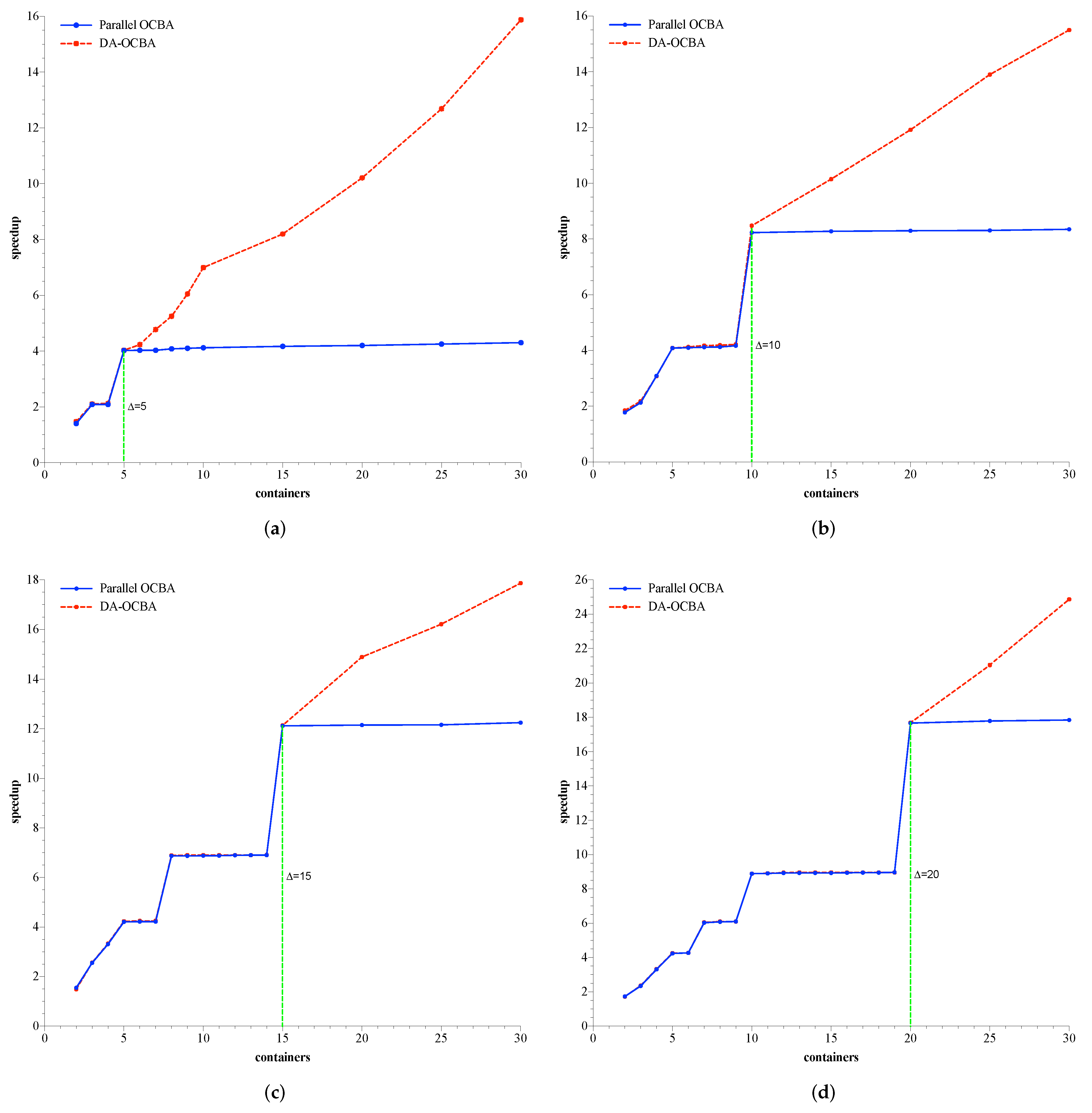
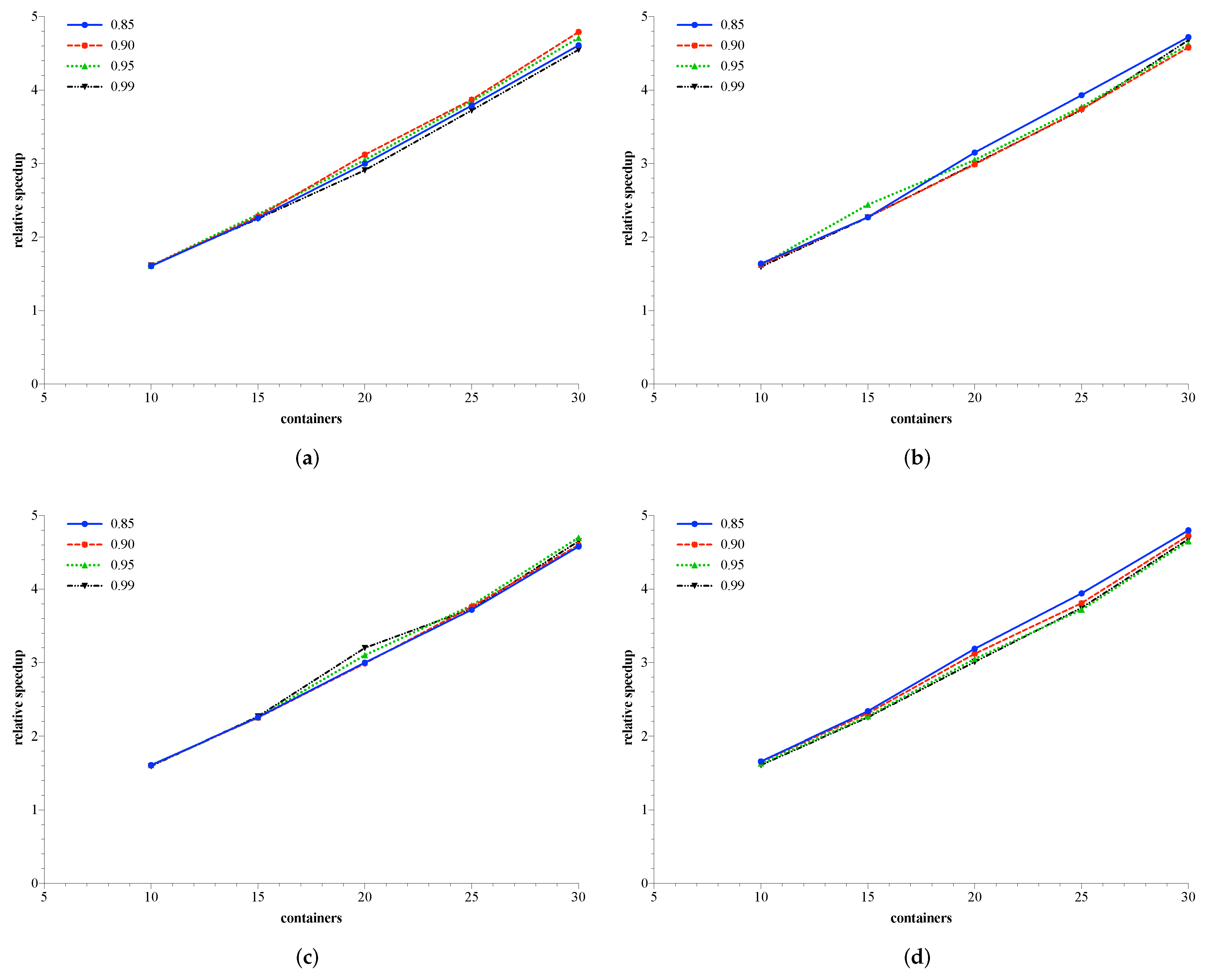
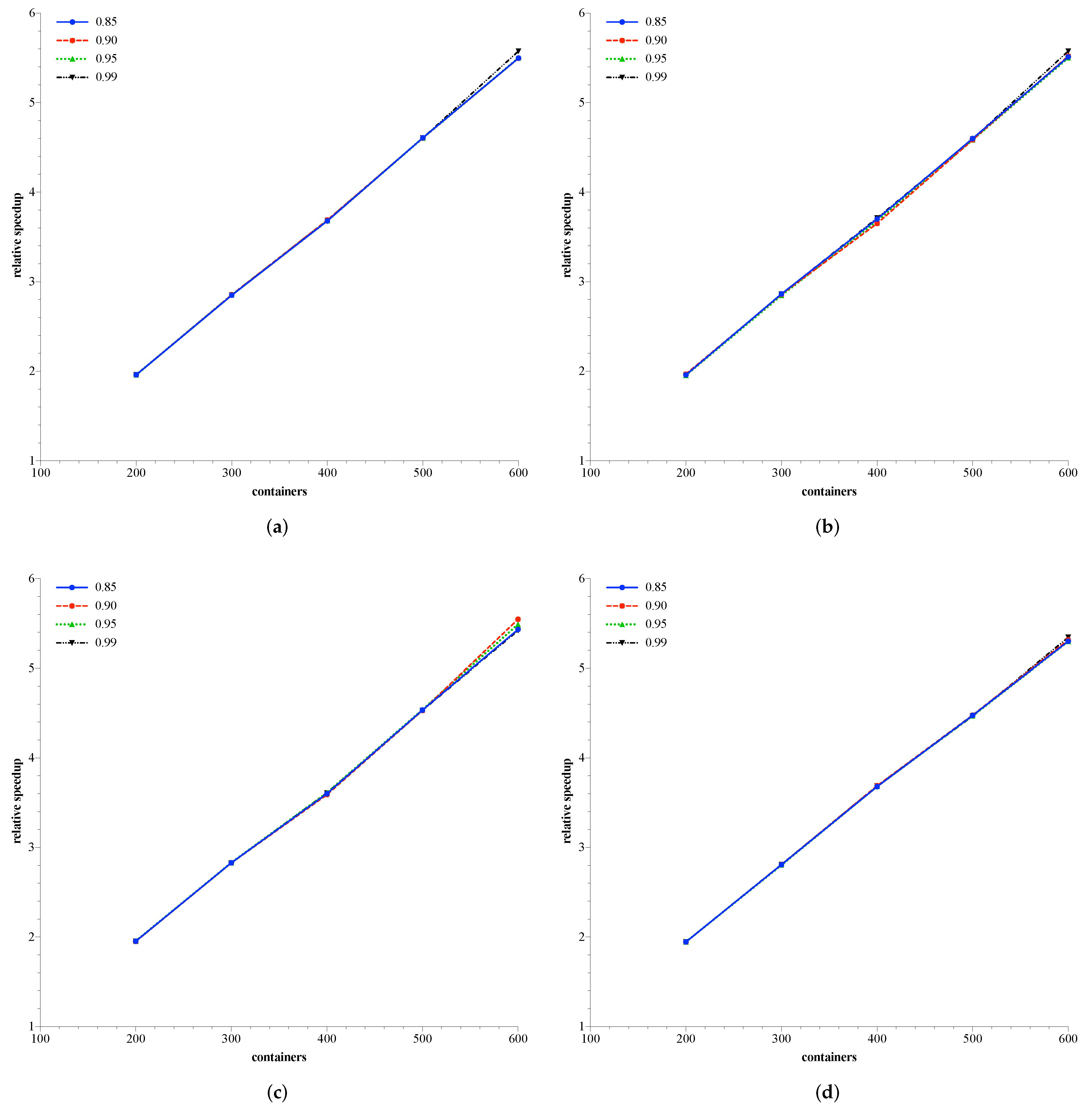
6.3. Relative Speedup of DA-OCBA

In order to show the relationship between speedup and number of containers for DA-OCBA, we used multiple and fewer designs to run the simulation. Only in this way could we get the exact relationship between them in different situations.

First, we set up a controlled trial for fewer designs, so that number of designs N = {5,10,15,20}. Each experiment with some designs had four $PCS$($PCS$ = {85%, 90%, 95%, 99%}); $\mathsf{\Delta }$ = 5; and initial number of simulations $n_0=5$. The relationship between the relative speedup and the number of containers is shown in Figure 5.

As is shown in Figure 5, the number of docker containers belongs to {10,15,20,25,30} that is an integer multiple of five containers. Here, $T_0$ is the total simulation time for five containers. With the number of containers linearly growing, the relative speedup of fewer designs for DA-OCBA was approximately linearly growing under four PCS. According to the polyline trend, we could obtain four asymptotes of different PCS for each subgraph in Figure 5 that had an approximate slope and the slope of all asymptotes for all subgraphs was approximate. That is because $\mathsf{\Delta }$ was equal between these four cases.

Second, we set up a controlled trial for multiple designs so that the number of designs was in N={1000, 1500, 2000, 2901}. Each experiment with some designs had four $PCS$($PCS$={85%, 90%, 95%, 99%}); $\mathsf{\Delta }$ = 100; and initial number of simulations $n_0=10$. The relationship between speedup and number of containers is shown in Figure 6.

As is shown in Figure 6, the number of docker containers belongs to {200,300,400,500,600} that is an integer multiple of 100 containers. Here, $t_0$ is the total simulation time for 100 containers. With the number of containers linearly growing, the speedup of fewer designs for DA-OCBA approximately linearly grows under four PCS. Again, the slope of all asymptotes for all subgraphs was also approximate. That is because $\mathsf{\Delta }$ was equal between these four cases.

However, it is obvious that the four lines of different PCS for each subgraph in Figure 6 were more fitting than Figure 5. This is because $\mathsf{\Delta }$ = 100 for multiple designs was more fine-grained than $\mathsf{\Delta }$ = 5 for fewer designs. For this reason, the change between four lines for four PCSs of fewer designs was bigger than that for multiple designs. Therefore, the stability of speedup under different PCS is determined by the granularity of $\mathsf{\Delta }$. The finer the granularity of $\mathsf{\Delta }$ is, the more stable the speedup is.

In summary, with the number of containers increasing, speedup grows linearly. The DA-OCBA compared with OCBA can take advantage of the sufficient computing resources and parallelism of cloud computing.

7. Conclusions and Future Work

This paper proposes a distributed asynchronous optimal computing budget allocation algorithm based on cloud platform Aliyun. This algorithm improves the efficiency of simulation optimization, and it solves the low utilization for the cloud by running designs in advance, such as parallelism, scalability, symmetry, and flexibility.The speedup of DA-OCBA is much larger than parallel OCBA. With the number of containers increasing, the DA-OCBA is getting higher and higher but the parallel OCBA is approximately unchanged. The DA-OCBA makes full use of cloud-computing resources, and the speedup of DA-OCBA is much higher than the parallel OCBA when there are enough containers. Therefore, the DA-OCBA is suitable for simulation optimization in a cloud environment, resulting in a great improvement in computational efficiency.

In the future, this algorithm will be tested for a larger number of designs and improved to maintain load balancing for designs of different scales. In order to try to meet multi-user Quality of Service (QoS) and to keep high speeds of simulation optimization, it is necessary to create an algorithm to ensure that some users will not delay running for too long. Meanwhile, there are differences in performance in the computing node in cloud computing and the communication overheads between each computing node and the management node are different. To improve the efficiency of simulation optimization, we need to create an algorithm that allocates multiple users to the most appropriate computing nodes. In summary, the ultimate goal is to build a cloud-based, highly efficient simulation optimization system that satisfies multi-user QoS.

References

1. Gosavi, A. Simulation-Based Optimization; Springer: Berlin/Heidelberg, Germany, 2015. [Google Scholar]
2. Fu, M.C. Handbook of Simulation Optimization; Springer: Berlin/Heidelberg, Germany, 2015; Volume 216. [Google Scholar]
3. Amaran, S.; Sahinidis, N.V.; Sharda, B.; Bury, S.J. Simulation optimization: A review of algorithms and applications. Ann. Oper. Res. 2016, 240, 351–380. [Google Scholar] [CrossRef]
4. Zhu, C.; Xu, J.; Chen, C.H.; Lee, L.H.; Hu, J.Q. Balancing search and estimation in random search based stochastic simulation optimization. IEEE Trans. Autom. Control 2016, 61, 3593–3598. [Google Scholar] [CrossRef]
5. Kleijnen, J.P. Design and analysis of simulation experiments. In International Workshop on Simulation; Springer: Berlin/Heidelberg, Germany, 2015; pp. 3–22. [Google Scholar]
6. Peng, Y.; Chen, C.H.; Chong, E.K.; Fu, M.C. A review of static and dynamic optimization for ranking and selection. In Proceedings of the 2018 Winter Simulation Conference (WSC), Gothenburg, Sweden, 9–12 December 2018; pp. 1909–1920. [Google Scholar]
7. Akl, A.M.; Sarker, R.A.; Essam, D.L. Simulation optimization approach for solving stochastic programming. In Proceedings of the 2017 2nd IEEE International Conference on Computational Intelligence and Applications (ICCIA), Beijing, China, 8–11 September 2017; pp. 161–165. [Google Scholar]
8. Gao, S.; Xiao, H.; Zhou, E.; Chen, W. Robust ranking and selection with optimal computing budget allocation. Automatica 2017, 81, 30–36. [Google Scholar] [CrossRef] [Green Version]
9. Chen, C.h.; Lee, L.H. Stochastic Simulation Optimization: An Optimal Computing Budget Allocation; World Scientific: Singapore, 2011; Volume 1. [Google Scholar]
10. Chen, C.H.; Yücesan, E.; Dai, L.; Chen, H.C. Optimal budget allocation for discrete-event simulation experiments. IIE Trans. 2009, 42, 60–70. [Google Scholar] [CrossRef]
11. Jian, N.; Henderson, S.G. An introduction to simulation optimization. In Proceedings of the 2015 Winter Simulation Conference (WSC), Huntington Beach, CA, USA, 6–9 December 2015; pp. 1780–1794. [Google Scholar]
12. Al-Salem, M.; Almomani, M.; Alrefaei, M.; Diabat, A. On the optimal computing budget allocation problem for large scale simulation optimization. Simul. Model. Pract. Theory 2017, 71, 149–159. [Google Scholar] [CrossRef]
13. Marinescu, D.C. Cloud Computing: Theory and Practice; Morgan Kaufmann: Burlington, MA, USA, 2017. [Google Scholar]
14. Chung, M.T.; Quang-Hung, N.; Nguyen, M.T.; Thoai, N. Using docker in high performance computing applications. In Proceedings of the 2016 IEEE Sixth International Conference on Communications and Electronics (ICCE), Ha Long, Vietnam, 27–29 July 2016; pp. 52–57. [Google Scholar]
15. DeHaan, M.P.; Henson, S.J.; Eckersberg, I.J.J. Flexible Cloud Management with Power Management Support. U.S. Patent 9,104,407, 2015. [Google Scholar]
16. Lee, L.H.; Chen, C.H.; Chew, E.P.; Li, J.; Zhang, S. A review of optimal computing budget allocation algorithms for simulation optimization problem. Int. J. Oper. Res. 2010, 7, 19–31. [Google Scholar]
17. Fu, M.C.; Glover, F.W.; April, J. Simulation optimization: A review, new developments, and applications. In Proceedings of the Winter Simulation Conference, Orlando, FL, USA, 4–7 December 2005; p. 13. [Google Scholar]
18. Dudewicz, E.J.; Dalal, S.R. Allocation of observations in ranking and selection with unequal variances. Optim. Methods Stat. 1975, 37, 28–78. [Google Scholar]
19. Rinott, Y. On two-stage selection procedures and related probability-inequalities. Commun. Stat. 1978, 7, 799–811. [Google Scholar] [CrossRef]
20. Nelson, B.L.; Swann, J.; Goldsman, D.; Song, W. Simple procedures for selecting the best simulated system when the number of alternatives is large. Oper. Res. 2001, 49, 950–963. [Google Scholar] [CrossRef]
21. Kim, S.H.; Nelson, B.L. A fully sequential procedure for indifference-zone selection in simulation. ACM Trans. Model. Comput. Simul. (TOMACS) 2001, 11, 251–273. [Google Scholar] [CrossRef]
22. Goldsman, D.; Nelson, B.L.; Banks, J. Comparing systems via simulation. In Handbook of Simulation: Principles, Methodology, Advances, Applications, and Practice; John Wiley & Sons: Hoboken, NJ, USA, 1998; pp. 273–306. [Google Scholar]
23. Law, A.M.; Kelton, W.D.; Kelton, W.D. Simulation Modeling and Analysis; McGraw-Hill: New York, NY, USA, 2000; Volume 3. [Google Scholar]
24. Kim, S.H.; Nelson, B. Selecting the best system: Simulation. In Elsevier Handbooks in Operations Research and Management Science: Simulation; Elsevier: Amsterdam, The Netherlands, 2006. [Google Scholar]
25. Chen, C.H.; Lin, J.; Yücesan, E.; Chick, S.E. Simulation Budget Allocation for Further Enhancing the Efficiency of Ordinal Optimization. Discret. Event Dyn. Syst. 2000, 10, 251–270. [Google Scholar] [CrossRef] [Green Version]
26. Chen, C.H.; Donohue, K.; Yücesan, E.; Lin, J. Optimal computing budget allocation for Monte Carlo simulation with application to product design. Simul. Model. Pract. Theory 2003, 11, 57–74. [Google Scholar] [CrossRef]
27. Lin, C.T.; Chen, J.; Jiang, W.J.; He, L.Y.W.; Shih, P.T.; Ho, C.H.; Chi, S. Ultra-High Data-Rate 60 GHz Radio-over-Fiber Systems Employing Optical Frequency Multiplication and Adaptive OFDM Formats. J. Lightwave Technol. 2010, 28, 2296–2306. [Google Scholar]
28. Glynn, P.; Juneja, S. A large deviations perspective on ordinal optimization. In Proceedings of the 36th Conference on Winter Simulation, Washington, DC, USA, 5–8 December 2004; pp. 577–585. [Google Scholar]
29. Bogon, T.; Timm, I.J.; Jessen, U.; Schmitz, M. Towards assisted input and output data analysis in manufacturing simulation: The EDASim approach. In Proceedings of the Winter Simulation Conference, Berlin, Germany, 9–12 December 2012; p. 257. [Google Scholar]
30. Laporte, G.J.; Branke, J.; Chen, C.H. Optimal computing budget allocation for small computing budgets. In Proceedings of the 2012 Winter Simulation Conference (WSC), Berlin, Germany, 9–12 December 2012. [Google Scholar]
31. Chen, C.H.; He, D.; Fu, M. Efficient dynamic simulation allocation in ordinal optimization. IEEE Trans. Autom. Control 2006, 51, 2005–2009. [Google Scholar] [CrossRef]
32. Ni, E.C.; Ciocan, D.F.; Henderson, S.G.; Hunter, S.R. Efficient Ranking and Selection in Parallel Computing Environments. Oper. Res. 2016, 65, 821–836. [Google Scholar] [CrossRef]
33. Radu, L.D. Green cloud computing: A literature survey. Symmetry 2017, 9, 295. [Google Scholar] [CrossRef]
34. Kim, S.H.; Nelson, B.L. Selecting the best system. Handb. Oper. Res. Manag. Sci. 2006, 13, 501–534. [Google Scholar]
35. Luo, J.; Hong, L.J. Large-scale ranking and selection using cloud computing. In Proceedings of the 2011 Winter Simulation Conference (WSC), Phoenix, AZ, USA, 11–14 December 2011; pp. 4046–4056. [Google Scholar]
36. Xu, J.; Huang, E.; Chen, C.H.; Lee, L.H. Simulation optimization: A review and exploration in the new era of cloud computing and big data. Asia-Pac. J. Oper. Res. 2015, 32, 1550019. [Google Scholar] [CrossRef]
37. Nelson, B.L. ‘Some tactical problems in digital simulation’for the next 10 years. J. Simul. 2016, 10, 2–11. [Google Scholar] [CrossRef]
38. Chick, S.E.; Inoue, K. New procedures to select the best simulated system using common random numbers. Manag. Sci. 2001, 47, 1133–1149. [Google Scholar] [CrossRef]
39. Law, A.M.; Kelton, W.D. Simulation Modeling and Analysis; McGraw-Hill: New York, NY, USA, 2009. [Google Scholar]
40. Lee, L.H.; Pujowidianto, N.A.; Li, L.W.; Chen, C.H.; Yap, C.M. Approximate Simulation Budget Allocation for Selecting the Best Design in the Presence of Stochastic Constraints. IEEE Trans. Autom. Control 2012, 57, 2940–2945. [Google Scholar] [CrossRef]
41. Chen, C.H.; Chen, H.C.; Dai, L. A gradient approach for smartly allocating computing budget for discrete event simulation. In Proceedings of the 28th Conference on Winter Simulation, Coronado, CA, USA, 8–11 December 1996; pp. 398–405. [Google Scholar]
42. Inoue, K.; Chick, S.E. Comparison of Bayesian and frequentist assessments of uncertainty for selecting the best system. In Proceedings of the 1998 Winter Simulation Conference, Washington, DC, USA, 13–16 December 1998. [Google Scholar]
43. Netto, H.V.; Lung, L.C.; Correia, M.; Luiz, A.F.; de Souza, L.M.S. State machine replication in containers managed by Kubernetes. J. Syst. Archit. 2017, 73, 53–59. [Google Scholar] [CrossRef]
44. Chen, H.C.; Chen, C.H.; Lin, J.; Yucesan, E. An asymptotic allocation for simultaneous simulation experiments. In Proceedings of the Conference on Winter Simulation: Simulation-a Bridge to the Future, Phoenix, AZ, USA, 5–8 December 1999. [Google Scholar]
45. Nakayama, M.K. Selecting the best system in steady-state simulations using batch means. In Proceedings of the 27th Conference on Winter Simulation, Arlington, VA, USA, 3–6 December 1995; pp. 362–366. [Google Scholar]
46. Koenig, L.W.; Law, A.M. A procedure for selecting a subset of size m containing the l best of k independent normal populations, with applications to simulation. Commun. Stat. -Simul. Comput. 1985, 14, 719–734. [Google Scholar] [CrossRef]
47. Boru, A.; Dosdoğru, A.T.; Göçken, M.; Erol, R. A Novel Hybrid Artificial Intelligence Based Methodology for the Inventory Routing Problem. Symmetry 2019, 11, 717. [Google Scholar] [CrossRef]
Figure 1. Docker running mechanism.
Symmetry 11 01297 g001
Figure 2. Distributed cloud platform.
Symmetry 11 01297 g002
Figure 3. Kubernetes framework.
Symmetry 11 01297 g003
Figure 4. Optimal computing budget allocation (OCBA) and distributed asynchronous OCBA (DA-OCBA) speedup. (a) Δ = 5 ; (b) Δ = 10 ; (c) Δ = 15 ; (d) Δ = 20 .
Symmetry 11 01297 g004
Figure 5. Relative speedup of fewer designs for DA-OCBA. Number of designs (N): (a) N = 5; (b) N = 10; (c) N = 15; and (d) N = 20.
Symmetry 11 01297 g005
Figure 6. Relative speedup of multiple designs for DA-OCBA. Number of designs (N): (a) N = 1000; (b) N = 1500; (c) N = 2000; and (d) N = 2901.
Symmetry 11 01297 g006