Article

Kinematics Modeling and Analysis of Mid-Low Speed Maglev Vehicle with Screw and Product of Exponential Theory

College of Intelligence Science and Technology, National University of Defense Technology, Changsha 410073, China
*
Author to whom correspondence should be addressed.
These authors contributed equally to this work.
Symmetry 2019, 11(10), 1201; https://doi.org/10.3390/sym11101201
Submission received: 20 August 2019 / Revised: 17 September 2019 / Accepted: 18 September 2019 / Published: 25 September 2019

Abstract

:
Maglev transportation is a new type of rail transit, whose vehicle is different from the two-bogie structure of the wheel-rail train. Generally, it consists of four to five suspension frames supporting a car body in parallel. The moving mechanism of a vehicle often consists of hundreds of moving parts, showing a multi-rigid body system in serial-parallel structure. At present, there is no theoretical framework for systematically and accurately describing the kinematics and dynamics of the Maglev train. The design work is at the level of simple equivalent estimation or measurement from the CAD drawing, which makes the system performance analysis and optimization work unable to be carried out scientifically. Based on the theoretical framework of screw theory and exponential mapping, the forward kinematics modeling, inverse kinematics solution, transition curve modeling and computational analysis methods for the Maglev train are proposed in this paper. A systematic and accurate theoretical framework is constructed for the modeling and analysis of the motion mechanism of the Maglev train, which makes the design and analysis of the Maglev train at the scientific level.

Graphical Abstract

1. Introduction

Maglev trains rely on non-contact electromagnetic forces to achieve contactless support. Compared with the traditional wheel-rail train, the Maglev train has the advantages of little mechanical wear, small vibration, stable operation, strong climbing ability, low noise, small turning radius and so on [1]. In recent years, with the commercial operation of the Changsha Maglev Express Line and the Beijing S1 Maglev Demonstration Line and the construction of the Qingyuan Line in Guangdong Province, the Maglev traffic has shown a rapid development momentum [2]. However, the kinematics and dynamics modeling analysis method of Maglev traffic lacks a unified and feasible theoretical framework. The design work is still at the level of simple equivalent estimation or drawing measurement. The lack of scientificity, completeness and accuracy restrict the progress of Maglev transportation technology.
The electromagnetic force required for the Maglev train is generated by the interaction between the vehicle electromagnet and the ferromagnetic track. In order to reduce the volume of the track and the system cost, the electromagnets and linear motors are generally arranged continuously along the length of the vehicle and the track. In addition, the suspension frame under one train is generally composed of four to five parallel arrangements. When the train is running, the plurality of suspension frames jointly support the train body in the form of a parallel mechanism, which makes the kinematics and dynamics analysis of the Maglev train different from that of the wheel-rail train supported by two bogies. Compared with the traditional wheel-rail train, the Maglev train has multiple suspension frames (multi-points) supporting the same body (a straight line), and each suspension frame presents different positions and attitudes relative to the body. Therefore, the kinematics and dynamics analysis of Maglev trains cannot inherit the existing theoretical framework of wheel-rail traffic.
There are more than 100 moving parts in each vehicle of a Maglev train, which presents a typical hybrid form of parallel mechanism and series mechanism. It is the goal of this paper to explore a theoretical method of analysis and synthesis to describe in detail the motion state of each moving mechanism of the vehicle. Based on the mathematical modeling theory of robotics, such as screw motion and exponential mapping, this paper establishes the mathematical modeling and analysis framework for the Maglev train motion mechanism, making the design and analysis of the Maglev train at a complete and accurate system level.
In the modeling method of mechanism kinematics, the D-H (Denavit-Hartenberg) transformation proposed by Denavit and Hartenberg [3,4] is a common method. However, in the equation of motion established by the D-H transform method [5], the Jacobian matrix, singularity analysis, etc. are related to the selection of the coordinate system of each component, which makes the analysis lose its generality. At the same time, the dynamic equations for establishing motion mechanisms based on D-H transformation are also quite complex. The application of helicoidal motion and exponential mapping in the mechanism [6] overcomes the above shortcomings. It is a perfect combination of rigid body motion, modern mathematics and classical mechanics. Furthermore, the helicoidal motion and exponential mapping [7,8] apply the concept of metric space on the manifold to the joint manifold of the motion mechanism, which makes the analysis and design of the mechanism more general. Therefore, it has become a universal modeling method for modern robotics.
In this paper, the forward kinematics modeling method of a mid-low speed Maglev train is introduced based on the theory of screw and exponential mapping. At the same time, the modeling method of the transition curve is analyzed, and the solution method of vehicle inverse kinematics is analyzed. Finally, based on the model established by the theory of screw and exponential mapping, an example of the solution of the motion mechanism in the Maglev train on the typical track of the transition curve is given.
The rest of the paper is organized as follows: Section 2 describes the forward kinematics modeling of mid-low speed Maglev trains. The solution of vehicle inverse kinematics is introduced in Section 3. In addition, the modeling of the track transition curve and the relationship of the vehicle/track posture is then introduced in Section 4. Section 5 presents the examples of motion based on the theory in the previous sections, which is followed by the conclusions in Section 6.

2. Forward Kinematics Modeling for a Mid-Low Speed Maglev Train

The running mechanism of the Maglev train mainly includes a suspension frame, a secondary suspension system (secondary system), an auxiliary steering mechanism and so on, as shown in Figure 1. Therefore, its kinematics modeling can be divided into two levels: the kinematics of the suspension frame and secondary kinematics. In the kinematics of the suspension frame, the left and right modules of the suspension frame are constrained by the track, so the kinematics mainly analyzes the movement of the anti-rolling beams and hanger rods inside the same suspension frame. The suspension frame in the mid-low speed Maglev train is mainly analyzed in this paper, and the analysis of the secondary system is similar to it.
The exponential mapping of series mechanism [6,9] is adopted to establish the forward kinematics model of the suspension frame. The front and rear anti-rolling mechanisms (including anti-rolling beam and hanger rod) in the suspension frame of the mid-low speed Maglev train are functionally symmetrical, forming a closed-chain parallel mechanism. Thus, the open-chain kinematics modeling method cannot directly be applied because of symmetrical motion, one set of anti-roll mechanisms can just be considered, and the motion of the other set of anti-roll mechanisms can be calculated symmetrically by this group. A front view of the suspension frame of a set of anti-roll mechanisms is shown as Figure 2.
As shown in Figure 2, the left module of the suspension frame is used as the base of the kinematic chain, and the reference is fixed to the base. Then, the degrees of freedom of the active joint between the left suspension module and the right suspension module are as follows:
(1)
There is a rotational degree of freedom along the z-direction between base 0 and anti-roll beam 1, whose twist coordinate is ξ 1 . This degree of freedom can decouple the motion of the left and right modules of the suspension frame in the running direction.
(2)
The ball joint between the anti-roll beam 1 and the hanger rod 2, respectively, includes three rotational degrees of freedom along x, y, and z. Considering the constraint relationship between the two anti-roll beams, the rotational degree of freedom in the z-direction can be ignored. Thus, the rotational degrees of freedom in the x- and y-directions are just considered, and the twists of rotation are ξ 3 and ξ 2 , respectively.
(3)
The hanger rod 2 has a telescopic translational freedom, and its twist is ξ 4 .
(4)
The ball joint between the anti-roll beam 1 and the hanger 2 respectively includes three rotational degrees of freedom. The degree of freedom in the z-direction is ignored, and the rotational freedom in the x-direction is retained and the twist is ξ 5 .
(5)
There is a rotational degree of freedom in the z-direction between the anti-roll beam 3 and the right module 4, whose twist coordinates are ξ 6 .
The above definition is shown in Figure 3.
According to the definition of spiral coordinates, ξ i = v i ω i R 6 . There is v i = ω i × q i for rotary joints, where ω i is the unit rotation axis and q i is any point on the rotation axis. For translational joints, ω i = 0 , and v i is the unit translation axis. According to Figure 3, the quantities are listed as: ω 1 = 0 0 1 T , q 1 = 0 0 0 T , ω 2 = 0 1 0 T , q 2 = 0 0 0 T , ω 3 = 1 0 0 T , q 3 = 0 l 1 0 T , ω 4 = 0 0 0 T , q 4 = 0 0 1 T , ω 5 = 1 0 0 T , q 5 = 0 l 1 l 2 T , ω 6 = 0 0 1 T , q 6 = 0 l 1 l 3 l 2 T . Then, the speed spiral coordinates of each link can be calculated. Let the rotation angle or translation distance of each joint be θ i , and the corresponding exponential mapping e ξ ^ θ can be calculated from the exponential mapping of the spiral coordinates:
e ξ ^ θ = e ω ^ θ I e ω ^ θ · ( ω × v ) + ω ω T v θ 0 1 .
It can be seen from Figure 3 that the initial posture of the right module T of the suspension frame relative to the reference frame J 0 is:
g J T ( 0 ) = 1 0 0 0 0 1 0 l 1 l 3 0 0 1 l 2 0 0 0 1 .
Thus, the forward kinematics equation for the suspension frame from the left module to the right module is
g J T ( θ ) = e ξ ^ 1 θ e ξ ^ 2 θ 2 e ξ ^ 3 θ 3 e ξ ^ 4 θ 4 e ξ ^ 5 θ 5 e ξ ^ 6 θ 6 g J T ( 0 ) .
Equation (3) is called the forward kinematics equation of the suspension frame, which is a 4 × 4 matrix:
g J T ( θ ) = n 11 n 12 n 13 p 1 n 21 n 22 n 23 p 2 n 31 n 32 n 33 p 3 0 0 0 1 .
Then, each element in Equation (4) through calculation is shown in Appendix A.
When the motion amount θ i of the joint in the suspension frame is known, the relative position and posture relationship between the left/right modules of the suspension frame can be calculated by Equation (3). On the contrary, the motion of each joint can also be calculated according to Equation (3) when the relative position and posture relationship between the left/right modules of the suspension frame is known. It is a basic tool for the design, analysis and verification of the suspension frame.

3. Solution of Reverse Motion of a Mid-Low Speed Maglev Train

The inverse solution of the kinematics is more important for the analysis and verification of the rationality of mechanism design. From the forward kinematics equation described by the exponential product and initial conditions, the inverse kinematics problem can be solved by two methods: the sub-problem method of exponential mapping [3,4] and the inverse transformation method of the robot kinematics solution [2]. The basic idea of these two methods is the same, that is, how to simplify the expressions on both sides of the equation and make the concise terms correspond equally. The ability to obtain an analytical form of kinematic inverse is a tricky job and requires certain conditions. In this paper, the inverse kinematics problem [10] of the suspension frame of the mid-low speed Maglev train is introduced.
The forward kinematics equation of the suspension frame in the Maglev train is formulated as Equation ( 3 ) . Assuming that the relative relationship between the left and right modules of the suspension frame is determined, in other words, the elements of the pose matrix G J T ( θ ) in Equation ( 4 ) are known. Let G J T ( θ ) = G J T . There are
e ξ ^ 1 θ 1 e ξ ^ 2 θ 2 e ξ ^ 3 θ 3 e ξ ^ 4 θ 4 e ξ ^ 5 θ 5 e ξ ^ 6 θ 6 = G J T · g J T 1 ( 0 ) .
The right side of Equation (5) is known. The transformation of Equation (5) is
e ξ ^ 1 θ 1 e ξ ^ 2 θ 2 e ξ ^ 3 θ 3 e ξ ^ 4 θ 4 e ξ ^ 5 θ 5 = G J T · [ g J T ( 0 ) ] 1 ( e ξ ^ 6 θ 6 ) 1 .
Let the first three rows of elements in the first column on the left side of the equation be equal to the corresponding elements on the right side, and the following equation is obtained:
cos θ 1 cos θ 2 = n 11 cos θ 6 n 12 sin θ 6 , sin θ 1 cos θ 2 = n 21 cos θ 6 n 22 sin θ 6 , sin θ 2 = n 31 cos θ 6 n 32 sin θ 6 .
According to Equation (5), the following equation can be obtained:
e ξ ^ 3 θ 3 e ξ ^ 4 θ 4 e ξ ^ 5 θ 5 e ξ ^ 6 θ 6 = ( e ξ ^ 1 θ 1 e ξ ^ 2 θ 2 ) 1 G J T · [ g J T ( 0 ) ] 1 .
According to the equal of the fourth column elements in the first row on the left and right sides in Equation (8), the equation can be obtained as follows:
( l 1 + l 3 ) sin θ 6 = p 3 sin θ 2 + p 1 cos θ 1 cos θ 2 + p 2 sin θ 1 cos θ 2 .
According to Equations (7) and (9), it can be found out
θ 6 = arctan p 1 n 11 + p 2 n 21 + p 3 n 31 p 1 n 12 + p 2 n 22 + p 3 n 32 l 1 l 3 .
By substituting θ 6 into Equation (7), it can be concluded that
θ 1 = arctan n 21 cos θ 6 n 22 sin θ 6 n 11 cos θ 6 n 12 sin θ 6 ,
θ 2 = arcsin n 31 cos θ 6 n 32 sin θ 6 .
According to Equation (7), we can obtain
e ξ ^ 3 θ 3 e ξ ^ 4 θ 4 e ξ ^ 5 θ 5 e ξ ^ 6 θ 6 = ( e ξ ^ 1 θ 1 e ξ ^ 2 θ 2 ) 1 G J T · [ g J T ( 0 ) ] 1 = Δ n 11 n 12 n 13 p 1 n 21 n 22 n 23 p 2 n 31 n 32 n 33 p 3 0 0 0 1 .
Thus, the variables θ 3 , θ 4 and θ 5 are obtained
θ 3 = arctan l 1 n 22 l 2 n 32 p 2 l 1 p 3 l 1 n 32 l 2 n 22 ,
θ 5 = arcsin 1 2 n 32 n 23 cos θ 3 n 22 + n 33 sin θ 3 ,
θ 4 = l 1 sin θ 5 + l 2 cos θ 5 1 p 3 cos θ 3 + l 1 + p 2 sin θ 3 .
Thus far, the analytical solution of the motion θ 1 θ 6 of the suspension frame is calculated. Therefore, the relative position and posture of the left and right modules in the suspension frame are used to obtain rotation or translation motion θ 1 θ 6 of six degrees of freedom in the internal anti-rolling mechanism.

4. The Relationship of the Vehicle/Track Position–Posture on the Transition Curve Track

4.1. Parametric Description of the Transition Curve

The transition curve is the transition section between the straight track and the circular track, usually in the form of gyration curve or sinusoidal curve. The main parameters which describe the transition curve are the curvature ρ ( s ) and transverse slope angle θ ( s ) . In addition, the total length of the transition curve S 0 , the maximum transverse slope angle θ 0 and the minimum radius R 0 of the transition curve are the boundary conditions of the transition curve.
The curvature and transverse slope angle of the gyration curve are linear functions of the track mileage s. The acceleration of the gyration curve is discontinuous. The vehicle has lateral impact at the end of the curve, which is suitable for the low-speed section.
The equation describing the transition curve is as follows:
ρ ( s ) = s R 0 S 0 , θ ( s ) = θ 0 s S 0 .
The curvature and transverse slope angle are defined, and the space equation of the center line of the transition curve can be given
d φ ( s ) d s = ρ ( s ) , d x ( s ) d s = cos φ ( s ) , d y ( s ) d s = sin φ ( s ) ,
where φ ( s ) is the direction angle of the transition curve, and ( x ( s ) , y ( s ) ) is at the orbital mileage s and the plane coordinate in the reference coordinate system whose coordinate origin is the starting point of the center line of the transition curve.
According to Equation (18), the algebraic equation of transition curve is obtained as follows:
y = x 3 6 S 0 R 0 + x 7 80 S 0 3 R 0 3 + O ( x 8 ) , s = x + x 5 40 S 0 2 R 0 2 + O ( x 8 ) .
Taking the first three approximations, the cubic parabolic approximation equation of the cycloid is obtained as follows:
x = s , y = x 3 6 S 0 R 0 .
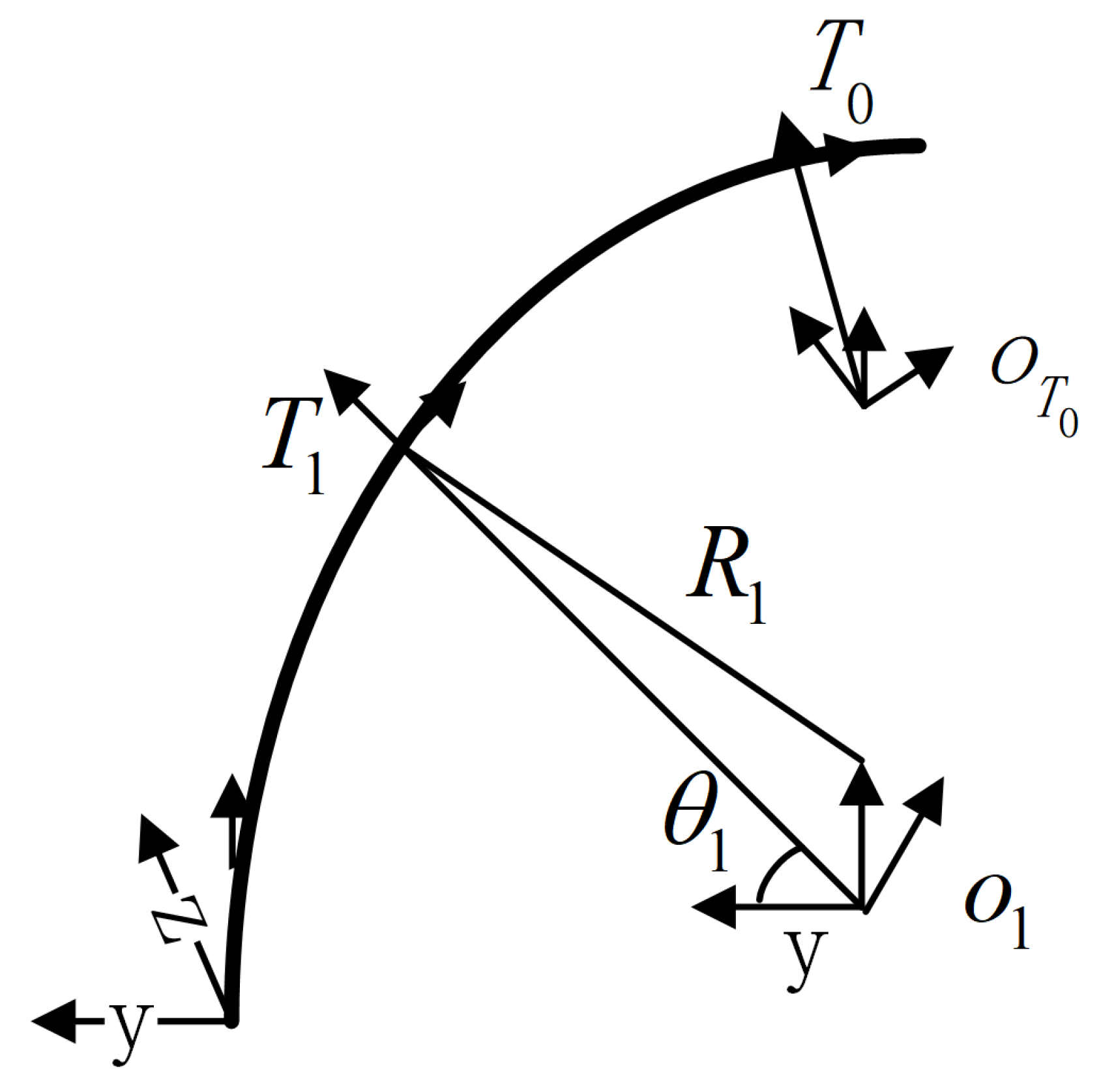
The rail surface formed by the transition curve is complex, and the center line is a kind of plane curve. In order to accurately describe the spatial posture of the transition curve, the coordinate system is defined as follows:The reference coordinate system O is located at the starting point of the center line of the transition curve. A moving coordinate system T 1 is set up on the track center line, which can move along the track center line. The other is the track reference coordinate system T 0 , which corresponds to the vehicle’s central coordinate system V 0 and has a relatively fixed position. The orbital mileage of their origins is respectively s 1 and s T 0 .
In order to get the posture matrix of the orbital coordinate system T R ( i ) , the posture matrix of T 1 relative to T 0 is calculated firstly. The auxiliary coordinate systems o 1 and o T 0 respectively corresponding to T 1 and T 0 are established. The origin of o 1 is located on the y-negative half axis of the T 1 , and the projection distance from the origin of T 1 is equal to the curvature radius R 1 at T 1 . The x-axis of o 1 is parallel to the x-axis of T 1 , and the z-axis is parallel to the z-axis of o 1 . In addition, the angle between the y-axis of T 1 and the y-axis is the transverse slope angle θ 1 . The definition of the coordinate system o T 0 is similar to that of o 1 . The coordinate systems are shown in Figure 4.
When the mileage s 1 is known, the coordinates of the origin of T 1 can be obtained from Equation (20):
T 1 = [ x 1 , y 1 , z 1 ] T = [ s 1 , s 1 3 6 S 0 R 0 , 0 ] T .
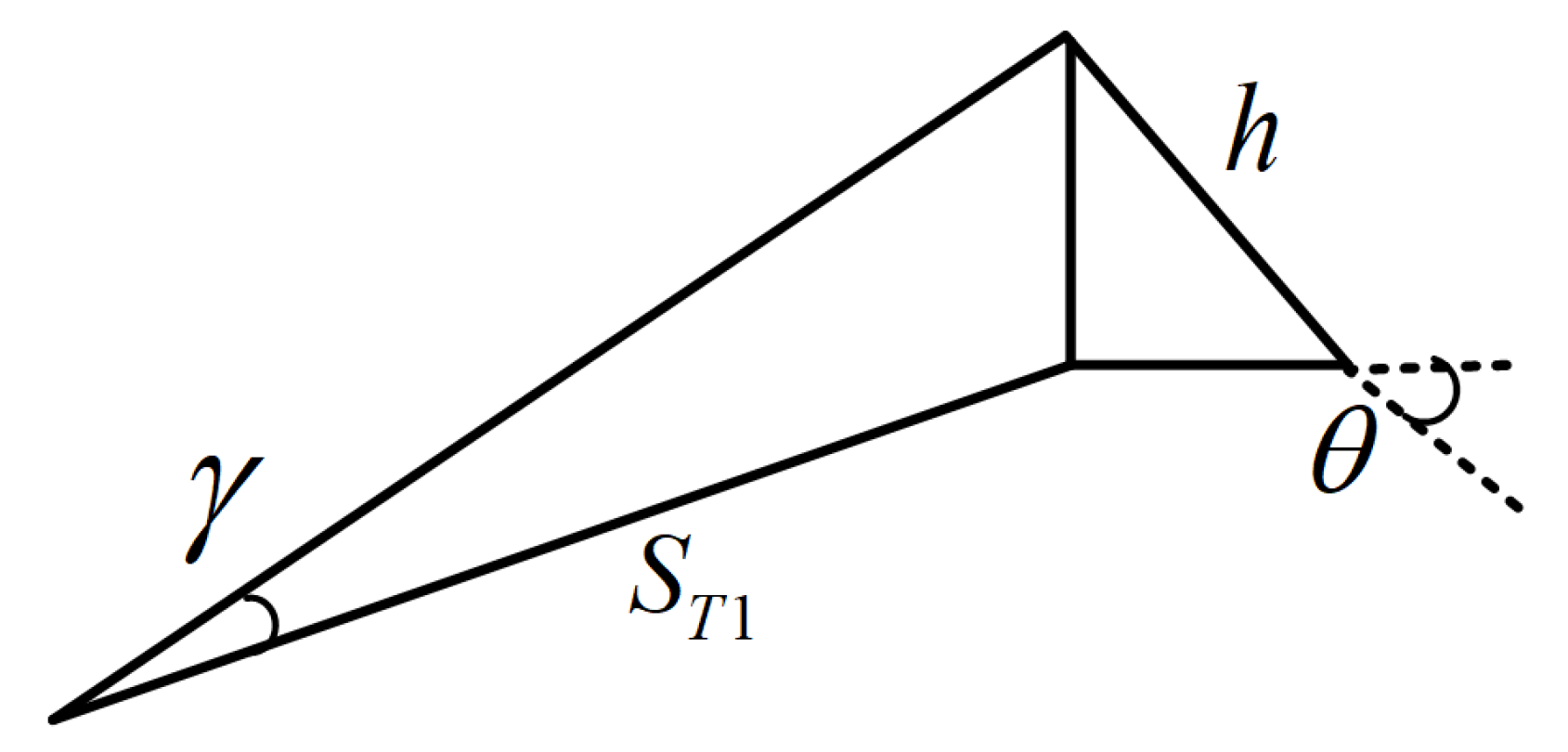
Considering that the orbit center line is a plane curve and parallel to the horizontal plane, the position vector of the coordinate origin of o 1 in the reference system O can be obtained from Figure 5:
o 1 O P = p 1 x p 1 y p 1 z = x 1 R c 1 sin φ 1 y 1 R c 1 cos φ 1 cos θ 1 R c 1 cos φ 1 sin θ 1 ,
where R c 1 = R 1 / cos θ 1 , R 1 is the radius of the curve at the origin of T 1 and φ 1 is the direction angle.
Since the z-axis of coordinate system o 1 is parallel to the z-axis of coordinate system O, the attitude of o 1 is formed by rotating φ 1 clockwise around the z-axis, so it has:
o 1 O R = R o t ( z , φ 1 ) = cos φ 1 sin φ 1 0 sin φ 1 cos φ 1 0 0 0 1 .
Then, the posture matrix of o 1 relative to O is obtained as follows:
o 1 O J = o 1 O R o 1 O P 0 1 = cos φ 1 sin φ 1 0 p 1 x sin φ 1 cos φ 1 0 p 1 y 0 0 1 p 1 z 0 0 0 1 .
Similarly, the posture matrix of o T 0 to O is obtained as follows:
o T 0 O J = cos ϕ T 0 sin ϕ T 0 0 p T 0 x sin ϕ T 0 cos ϕ T 0 0 p T 0 y 0 0 1 p T 0 z 0 0 0 1 .
Furthermore, the equation of the posture matrix of o 1 to o T 0 is obtained as follows:
o 1 o T 0 J = ( o T 0 O J ) 1 o 1 O J = cos ( ϕ T 0 ϕ 1 ) sin ( ϕ T 0 ϕ 1 ) 0 ( p T 0 x p 1 x ) cos ϕ T 0 + ( p T 0 y p 1 y ) sin ϕ T 0 sin ( ϕ T 0 ϕ 1 ) cos ( ϕ T 0 ϕ 1 ) 0 ( p T 0 x p 1 x ) sin ϕ T 0 ( p T 0 y p 1 y ) cos ϕ T 0 0 0 1 ( p T 0 z p 1 z ) 0 0 0 1 .
After setting the auxiliary coordinate systems o 1 and o T 0 , the posture matrix of T 1 in coordinate system o 1 can be easily obtained:
T 1 o 1 J = 1 0 0 0 0 cos θ 1 sin θ 1 R 1 0 sin θ 1 cos θ 1 R 1 tan θ 1 0 0 0 1 .
Similarly, the posture matrix of T 1 in coordinate system o T 0 can be obtained:
T 0 o T 0 J = 1 0 0 0 0 cos θ T 0 sin θ T 0 R T 0 0 sin θ T 0 cos θ T 0 R T 0 tan θ T 0 0 0 0 1 .
According to Equations (26)–(28), the posture matrix of the coordinate system T 1 to the fixed coordinate system T 0 can be obtained:
T 1 T 0 J = ( T 0 o T 0 J ) 1 · o 1 o T 0 J · T 1 o 1 J .
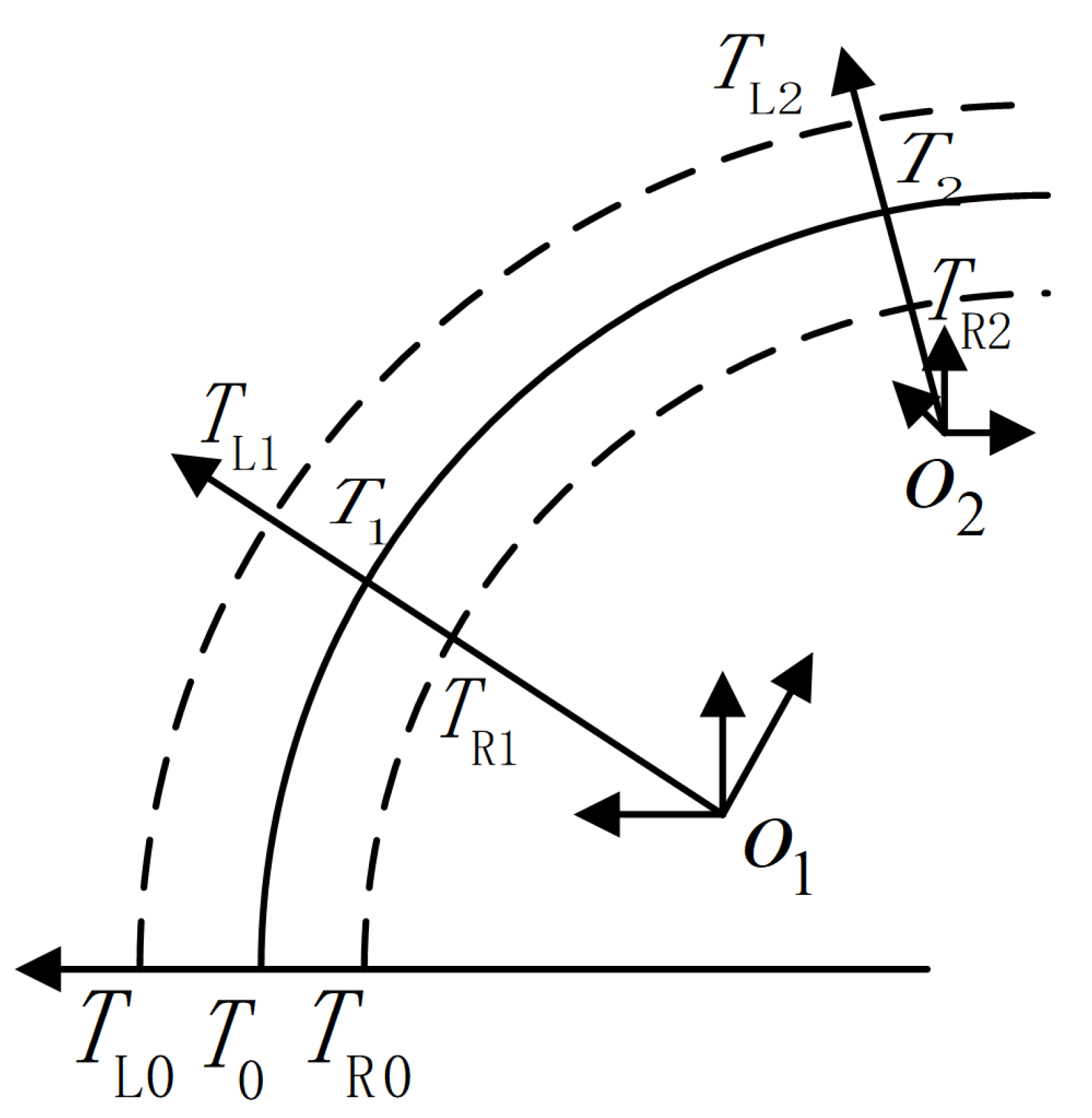
The relative posture relations of T 1 and T 0 cannot directly reflect the posture relations of both sides of the track. For this reason, the coordinate system T L 1 is established on the left track of the transition curve corresponding to the center line coordinate system T 1 , and the coordinate system T R 1 is established on the right track. The characteristics of the transition curve determine that the origins of T R 1 and T L 1 are located on the y-axis of the T 1 coordinate system, and the distance from the origin of T 1 is, respectively, ± 1 2 D (D is gauge). The coordinate system is shown in Figure 6.
As for attitude, the x-axis of T R 1 is along the tangent direction of the right side rail and the x-axis of T L 1 is along the tangent direction of the left side rail. There is an angle between them and the x-axis of T 1 . The spatial relationship is shown in Figure 5.
The angle γ can be approximated to the ratio between the track super high h and the mileage s:
γ = h s T 1 = D 2 sin θ 1 s T 1 D 2 θ 1 s T 1 = D 2 θ 0 s T 1 S 0 s T 1 = D θ 0 2 S 0 .
When the parameters of the transition curve are determined, h is a constant. Thus, the posture matrix of T R 1 relative to T 1 can be obtained as follows:
T R 1 T 1 J = cos γ 0 sin γ 0 0 1 0 1 2 D sin γ 0 cos γ 0 0 0 0 1 .
By combining Equation (29) with Equation (31), it can be obtained:
T R 1 T 0 J = T 1 T 0 J · T R 1 T 1 J .
Similarly, the posture matrix T L 1 T 1 J of T L relative to T 1 is obtained:
T L 1 T 1 J = cos γ 0 sin γ 0 0 1 0 1 2 D sin γ 0 cos γ 0 0 0 0 1 .
By combining Equation (29) with Equation (33), it can be obtained:
T L 1 T 0 J = T 1 T 0 J · T L 1 T 1 J .
Equations (32) and (34) are the posture matrices of the track coordinate system relative to the track reference coordinate system.

4.2. The Track Coordinate System on the Transition Curve

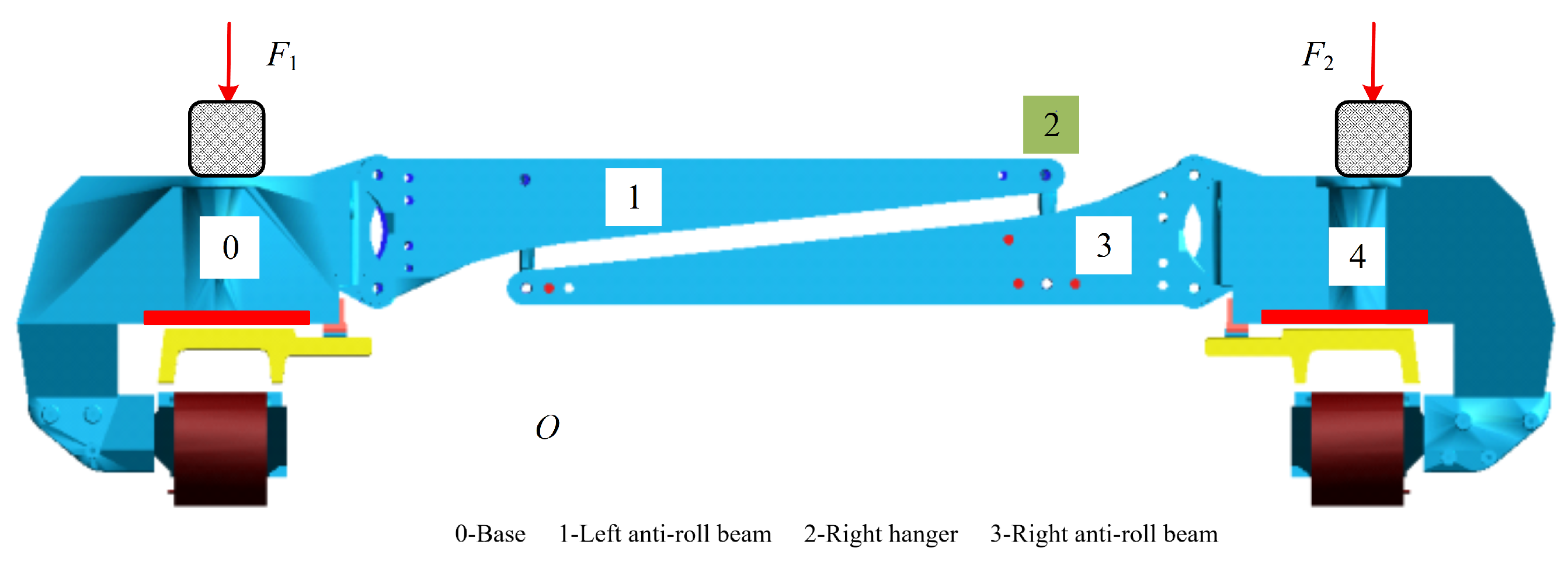
The left/right tracks of the transition curve are not coplanar, and their common role determines the motion of the vehicle. At the same time, the radius of curvature and the transverse slope angle of each point on the transition curve are different. When the track is close to the end of the circular curve, its radius of curvature is the smallest and the angle of transverse slope is the largest, which is the part that requires more stringent vehicle structure. Therefore, this paper puts the vehicle at this end for analysis.
Generally speaking, the length of the electromagnet is about several meters, while the radius of the transition curve and circular curve is about 100–1000 m. Therefore, the error of replacing the arc length (mileage) of the track with the space distribution length of the electromagnet can be neglected. 
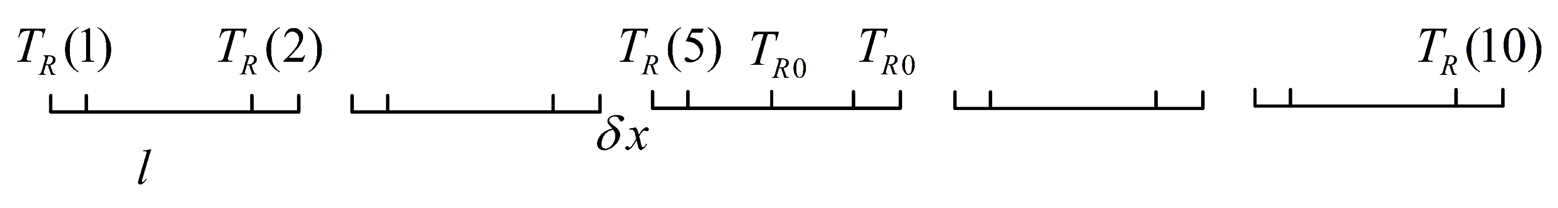
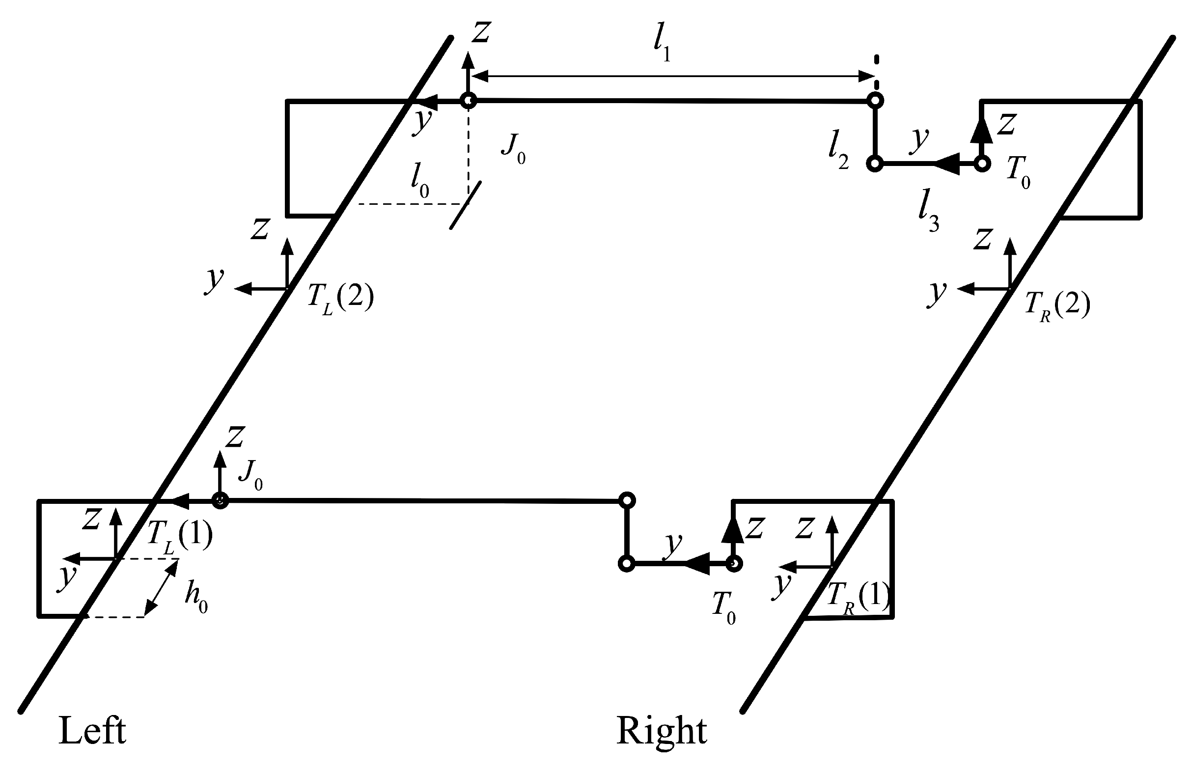
Figure 7 shows the spatial relationship between the electromagnets on both sides of the vehicle and the track.
In Figure 7, l is the length of the electromagnet and δ x is the distance between adjacent suspension frames. Taking the right side as an example, with the first coordinate system T R ( 1 ) as the starting point, the distance between 10 l and T R ( 1 ) is as follows:
s T ( i ) = 1 2 l × ( i 1 ) + δ x × c e i l ( i 2 2 ) i = 1 , 2 , , 10 ,
where i denotes the label of the coordinate system T R ( i ) and c e i l ( · ) is the upward rounding function.
The parameter i = 10 is brought into Equation (35), and the span between the coordinate system T R ( 1 ) and T R ( 10 ) is calculated as s v e h i c l e = 4.5 l + 4 δ x . If the total length of the transition curve is S 0 , the starting point of the mileage of T ( 1 ) is set to S 0 s v e h i c l e . Thus, the mileage of each T ( i ) relative to the reference system O becomes:
s T ( i ) = 1 2 l × ( i 1 ) + δ x × c e i l ( i 2 2 ) + S 0 s v e h i c l e i = 1 , 2 , , 10 .
On the right side of the vehicle, the mileage of five electromagnet midpoints to the reference system O becomes:
s M ( k ) = ( l + δ x ) × ( k 1 ) + l / 4 + S 0 s v e h i c l e k = 1 , 2 , , 5 .
The track reference coordinate system T 0 is located at the midpoint of the vehicle body span mileage on the track center line. Its mileage is:
s T 0 = 2 ( l + δ x ) + l / 4 + S 0 s v e h i c l e = S 0 2.25 l 2 δ x .
According to Equations (36) and (37), the position vector of T ( i ) relative to T 0 can be obtained as follows:
T 0 P ( i ) = ( p 1 x p T 0 x ) c ϕ T 0 ( p 1 y p T 0 y ) s ϕ T 0 + R 1 s ( ϕ ( i ) ϕ T 0 ) ( p 1 z p T 0 z ) s θ T 0 + [ ( p 1 x p T 0 x ) s ϕ T 0 + ( p 1 y p T 0 y ) c ϕ T 0 + R 1 c ( ϕ ( i ) ϕ T 0 ) ] c θ T 0 + R 1 s θ T 0 t θ ( i ) R T 0 / c θ T 0 ( p 1 z p T 0 z ) c θ T 0 [ ( p 1 x p T 0 x ) s ϕ T 0 + ( p 1 y p T 0 y ) c ϕ T 0 + R 1 c ( ϕ ( i ) ϕ T 0 ) ] s θ T 0 + R 1 c θ T 0 t θ ( i ) .
By introducing Equations (37) and (38) into Equation (29), the posture matrix of the mid-point of five electromagnets is obtained as follows:
T 0 R ( k ) = c ( ϕ ( k ) ϕ T 0 ) s ( ϕ ( k ) ϕ T 0 ) c θ T 0 s ( ϕ ( k ) ϕ T 0 ) s θ T 0 s ( ϕ ( k ) ϕ T 0 ) c θ T 0 s θ 1 s θ T 0 + c ( ϕ ( k ) ϕ T 0 ) c θ 1 c θ T 0 c θ 1 s θ T 0 c ( ϕ ( k ) ϕ T 0 ) s θ 1 c θ T 0 s ( ϕ ( k ) ϕ T 0 ) s θ T 0 s θ 1 c θ T 0 c ( ϕ ( k ) ϕ T 0 ) c θ 1 s θ T 0 c θ 1 c θ T 0 + c ( ϕ ( k ) ϕ T 0 ) s θ 1 s θ T 0 .
By Equations (39) and (40), the posture matrix of T ( i ) relative to track reference coordinate system T 0 is obtained as follows:
T 0 T ( i ) = T 0 R ( k ) T 0 P ( i ) 0 1 i = 1 , , 10 ; k = c e i l ( i 2 ) .
Similarly, the posture matrix of T R ( i ) relative to track reference coordinate system T 0 can be expressed as:
T R ( i ) T 0 J = T 0 T ( i ) · T R 1 T 1 J = T 0 R ( k ) T 0 P ( i ) 0 1 · T R 1 T 1 J i = 1 , , 10 ; k = c e i l ( i 2 ) .
Thus, the posture matrix of T R ( i ) relative to track reference coordinate system T 0 can be also expressed as:
T L ( i ) T 0 J = T 0 T ( i ) · T L 1 T 1 J = T 0 R ( k ) T 0 P ( i ) 0 1 · T L 1 T 1 J i = 1 , , 10 ; k = c e i l ( i 2 ) .
The posture relationship of the right track coordinate system with respect to the left track coordinate system is:
T R ( i ) T L ( i ) J = T L ( i ) T 0 J 1 T R ( i ) T 0 J .

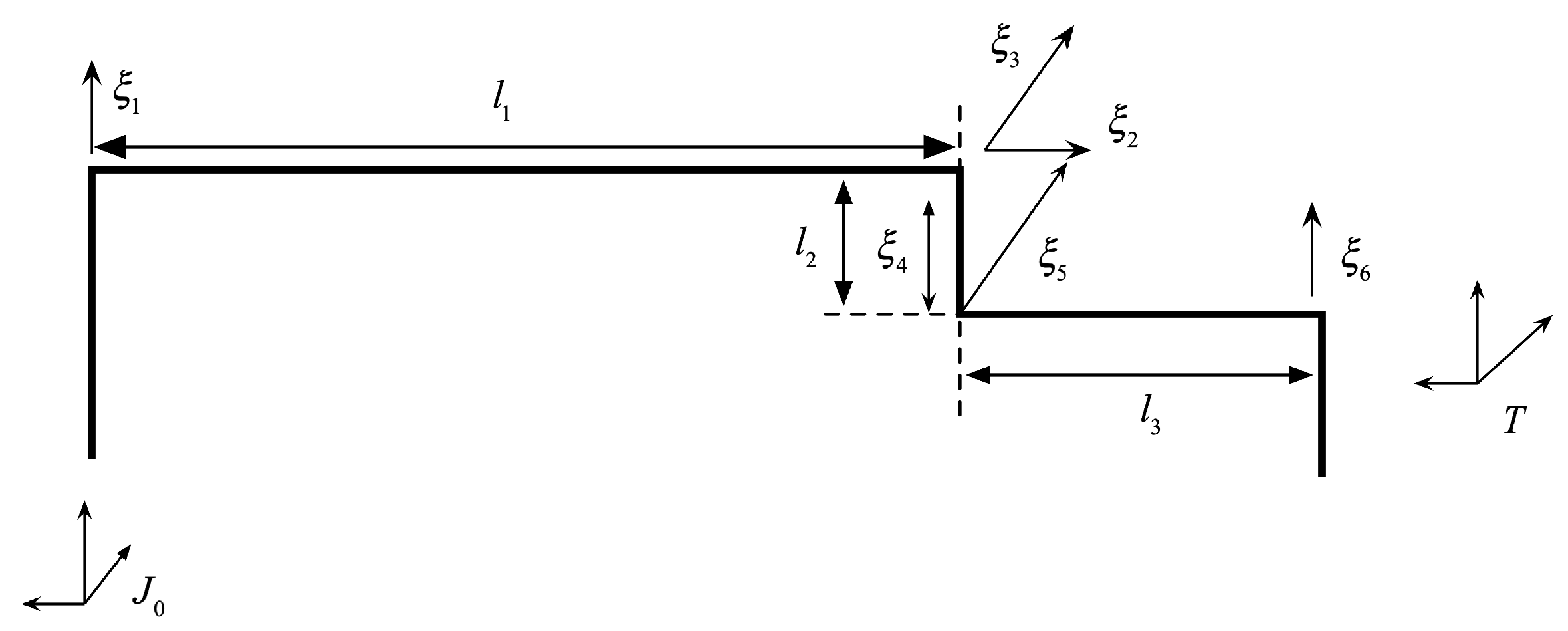
4.3. The Posture Matrix of Train Reference System V 0 Relative to Track Reference System T 0

The curvature of the transition curve changes with the length gradually, and the relative relationship between the front/rear of the train body and the track is asymmetric. However, the relative motion of electromagnet and train body in the horizontal direction (
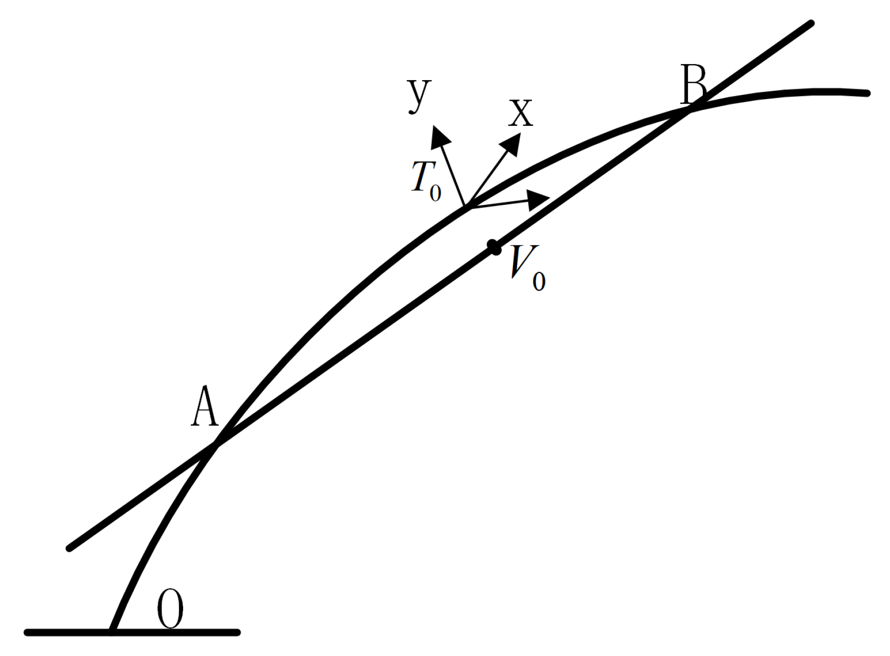
y-direction) is limited by the rotating sliding table between the suspension frames 1(4) and suspension frames 2(5) on the train body. This paper analyses the movement of the vehicle to the large curvature end of the transition curve. The relative relationship between the train and the transition curve is shown in Figure 8.
In Figure 8, the length of A B can be calculated from the structure of the vehicle:
L A B = 3 l + 3 δ x .
According to Equation (38), the mileage of A and B are:
s A = s T 0 1 2 L A B = S 0 3.75 l 3.5 δ x ,
s B = s T 0 + 1 2 L A B = S 0 0.75 l 0.5 δ x .
The position vectors P A = ( x A , y A , z A ) T and P B = ( x B , y B , z B ) T of A and B can be obtained by using Equation (29). At the same time, the body reference system V 0 is located at the midpoint of the line segment A B , so the position vector of V 0 in T 0 is:
P V 0 = ( x A + x B 2 , y A + y B 2 , z A + z B 2 + h 0 ) T .
Note: The nominal height h 0 of the secondary system with the difference in the z-direction between V 0 and T 0 is directly added to the third term of Equation (48).
Because of the balance of forces, it is generally believed that the posture of the body reference system is the same as that of the track reference system. Therefore, the posture matrix of V 0 in T 0 can be obtained as follows:
V 0 T 0 J = I 3 × 3 P V 0 0 1 .
Thus far, the posture matrix of the train body constrained coordinate system V R ( i ) and V L ( i ) relative to the track constrained coordinate system T R ( i ) and T L ( i ) are obtained:
V R ( i ) T R ( i ) J = T 0 T R ( i ) J × V 0 T 0 J × V R ( i ) V 0 J = [ T R ( i ) T 0 J ] 1 × V 0 T 0 J × V 0 V R ( i ) ,
V L ( i ) T L ( i ) J = T 0 T L ( i ) J × V 0 T 0 J × V L ( i ) V 0 J = [ T L ( i ) T 0 J ] 1 × V 0 T 0 J × V 0 V L ( i ) .
In Equations (50) and (51), T R ( i ) T 0 J and T L ( i ) T 0 J are determined by Equations (42) and (43), V 0 T 0 J is determined by Equation (49), and V 0 V R ( i ) and V 0 V L ( i ) can be obtained by the posture matrix of the coordinate system in the left/right sliding table relative to that of the reference coordinate system in the train body.
The posture matrix V R ( i ) T R ( i ) J and V L ( i ) T L ( i ) J describes the posture relationship from the train-constrained coordinate system to the track-constrained coordinate system, and also determines the motion of the suspension frame and the secondary system. Using these pose matrices, the motion range of the secondary system, suspension frame and other parts in the train can be calculated, which provides an accurate basis for the design.

5. The Motion Analysis of the Maglev Train

The inverse kinematics equations of suspension frame and secondary system are established in Section 3, and the constraint matrix from the body coordinate system to track coordinate system is established. In this section, the motion of suspension frame in the Maglev train on the transition curve is taken as an example, and the calculation results of specific motion range are given.
The reference coordinate systems J 0 and T 0 of the kinematics equation of the suspension frame are set at the first joint of the anti-rolling beam group (the connection between the left module and the anti-rolling beam) and the last joint (the connection between the right module and the anti-rolling beam). They do not coincide with the track coordinate system T L ( i ) and T R ( i ) . Therefore, it is necessary to design the transformation matrix so as to transform the train–track constraint relation to the reference system of the inverse kinematics solution.
The spatial relationship between the suspension module and the electromagnet corresponding to a suspension frame is shown in Figure 9.
It can be seen in Figure 9 that the postures of the reference coordinate system and the terminal coordinate system of the suspension frame are the same as that of the orbit coordinate system, but the origin does not coincide.
h 0 : The distance from the origin of the track coordinate system T L ( i ) T R ( i ) on the center line of the electromagnet polar surface to the cross section of the anti-rolling beam group (x-direction of the reference system);
h 1 : The vertical distance from the pole surface of the electromagnet to the upper hinge (z-direction of the reference system);
l 0 : The distance from the polar axis of the electromagnet to the anti-roll beam and the module hinge (y-axis of the reference system);
The definitions of l 1 , l 2 and l 3 are given in Section 2 of the kinematic modeling of the suspension frame.
The parameters of the transition curve and the Maglev train are shown in Table 1.
As can be seen from Figure 9, for the right module of the suspension frame, the transformation matrix from the terminal coordinate system T 0 of the suspension frame to the track coordinate system T R ( i ) is as follows:
T 0 ( i ) T R ( i ) J = 1 0 0 ( 1 ) i h 0 0 1 0 l 0 0 0 1 h 1 l 2 0 0 0 1 .
In Equation (52), the l 2 is the height difference between the terminal coordinate system and the reference coordinate system.
On the left module, the transformation matrix from the reference coordinate system J 0 to the orbit coordinate system T L ( i ) is as follows:
J 0 ( i ) T L ( i ) J = 1 0 0 ( 1 ) i h 0 0 1 0 l 0 0 0 1 h 1 0 0 0 1 .
Thus, the posture transformation relationship from the right track coordinate system to the left track coordinate system is as follows:
T R ( i ) T L ( i ) J = J 0 ( i ) T L ( i ) J × T 0 ( i ) J 0 ( i ) J × T R ( i ) T 0 ( i ) J
so
T 0 ( i ) J 0 ( i ) J = J 0 ( i ) T L ( i ) J 1 × T R ( i ) T L ( i ) J × T 0 ( i ) T R ( i ) J .
In Equation (55), the first term is determined by Equation (53), the second is decided by Equation (44), and the third is determined by Equation (52). The T o ( i ) J o ( i ) J calculated on the left side is the constraint matrix of the posture relationship between the two ends of the suspension frame, which is brought into the inverse kinematics equation of the suspension frame to calculate the motion of each joint of the anti-rolling beam group.
According to the parameters of transition curve, the joint motion of 10 anti-rolling beam groups on five suspension frames of vehicle is simulated as shown in Table 2.
From the data in Table 2, it can be seen that the range of motion joints in the anti-rolling beam group changes: θ 1 0.6 , θ 2 0.5 , θ 3 0 , θ 4 6 m m , θ 5 0 , θ 6 0.6 . It can be seen that, under the premise that the suspension module follows the track strictly, when the suspension frame passes through the transition curve (the minimum radius is 100 m, the maximum superelevation is 6 degrees), the suspension frame hanger rod needs about 6 mm expansion. The data obtained by the simulation can provide reliable data for the design of the suspension frame, and can carry out quantitative analysis and calculation, which greatly improves the reliability and stability of the design structure.

6. Conclusions

In this paper, the differentiable manifold, Lie group, Lie algebra and screw theory in the field of rigid body motion are applied to the kinematics modeling and analysis about Maglev train and track for the first time, which provides a systematic and scientific theoretical framework for the kinematics/dynamics modeling and analysis in the Maglev traffic. The method introduced in this paper can study the kinematics of the system from the macroscopic point of the train and track. It can change the status that the design and analysis is from bottom to top for many years, and hopefully raise the technology of Maglev transportation to the scientific level. Based on the research and development experience of Maglev transportation technology for many years, the conclusions obtained in this paper have been verified by practice, which proves the effectiveness and superiority of the proposed theoretical method.

Author Contributions

Conceptualization, P.L. and J.L.; validation, P.L., J.L. and Y.J.; writing—original draft preparation, P.L.; writing—review and editing, J.L. and Y.J.; supervision, J.L.

Funding

This research was funded by the National Key R&D Program of China (Grant No. 2016YFB1200601).

Conflicts of Interest

The authors declare no conflict of interest.

Appendix A

Appendix A.1. Each Element in Equation (4)

n 11 = c θ 1 c θ 2 c θ 6 s θ 6 c θ 5 s θ 1 c θ 3 + c θ 1 s θ 2 s θ 3 s θ 5 s θ 1 s θ 3 c θ 1 s θ 2 c θ 3 ,
n 12 = c θ 1 c θ 2 s θ 6 c θ 6 c θ 5 s θ 1 c θ 3 + c θ 1 s θ 2 s θ 3 s θ 5 s θ 1 s θ 3 c θ 1 s θ 2 c θ 3 ,
n 13 = c θ 5 s θ 1 c θ 3 c θ 1 s θ 2 c θ 3 + s θ 5 s θ 1 c θ 3 + c θ 1 s θ 2 s θ 3 ,
p 1 = l 1 s θ 1 ( l 2 + θ 4 ) s θ 1 s θ 3 + l 2 c θ 1 s θ 2 c θ 3 + l 3 s θ 1 c θ 3 s θ 5 s θ 3 s θ 5 + θ 4 c θ 1 s θ 2 c θ 3 + l 3 c θ 1 s θ 2 c θ 3 s θ 5 + s θ 3 c θ 5 ,
n 21 = s θ 1 c θ 2 c θ 6 s θ 6 c θ 5 c θ 1 c θ 3 s θ 1 s θ 2 s θ 3 s θ 5 c θ 1 s θ 3 s θ 1 s θ 2 c θ 3 ,
n 22 = s θ 1 c θ 2 s θ 6 + c θ 6 c θ 5 c θ 1 c θ 3 s θ 1 s θ 2 s θ 3 s θ 5 c θ 1 s θ 3 + s θ 1 s θ 2 c θ 3 ,
n 23 = c θ 5 c θ 1 s θ 3 + s θ 1 s θ 2 c θ 3 s θ 5 c θ 1 c θ 3 s θ 1 s θ 2 s θ 3 ,
p 2 = l 1 c θ 1 + ( l 2 + θ 4 ) c θ 1 s θ 3 + l 2 s θ 1 s θ 2 c θ 3 l 3 c θ 1 c θ 3 s θ 5 s θ 3 s θ 5 + θ 4 s θ 1 s θ 2 c θ 3 + l 3 s θ 1 s θ 2 c θ 3 s θ 5 + s θ 3 c θ 5 ,
n 31 = s θ 2 c θ 6 + s θ 6 c θ 2 c θ 3 s θ 5 + c θ 2 s θ 3 c θ 5 ,
n 32 = s θ 2 s θ 6 + c θ 6 c θ 2 c θ 3 s θ 5 + c θ 2 s θ 3 c θ 5 ,
n 33 = c θ 2 c ( θ 3 + θ 5 ) ,
p 3 = c θ 2 l 3 s ( θ 3 + θ 5 ) + l 2 c θ 3 + θ 4 c θ 3 .

References

  1. Youlun, X. Science of Robotics; China Machine Press: Beijing, China, 1992. [Google Scholar]
  2. Zixing, C. Robotics: Principles and Applications; South and Center University Press: Changsha, China, 1988. [Google Scholar]
  3. Murray, R.; Zexiang, L.; Sastry, S. A Mathematical Introduction to Robotic Manipulation; CRC Press: Boca Raton, FL, USA, 2005. [Google Scholar]
  4. Jingjun, D.; Xinjun, L.; Xilun, D. Mathematic Foundation of Mechanisms and Robotics, 2nd ed.; Machine Press: Beijing, China, 2016. [Google Scholar]
  5. Santolaria, J.; Aguilar, J.-J.; Yagüe, J.-A.; Pastor, J. Kinematic parameter estimation technique for calibration and repeatability improvement of articulated arm coordinate measuring machines. Precis. Eng. 2008, 32, 251–268. [Google Scholar] [CrossRef]
  6. Jie, L.; Tijian, S.; Kun, Z. Kinematical Analysis for the Second Suspension System of the Maglev Vehicle. J. China Railw. Soc. 2007, 29, 32–38. [Google Scholar]
  7. Fernandez-Gauna, B.; Lopez-Guede, J.M.; Zulueta, E.; Echegoyen, Z.; Graña, M. Basic results and experiments on robotic multi-agent system for hose deployment and transportation. Int. J. Artif. Intell. 2011, 6, 183–202. [Google Scholar]
  8. Takács, Á.; Kovács, L.; Rudas, I.; Precup, R.-E.; Haidegger, T. Models for force control in telesurgical robot systems. Acta Polytech. Hung. 2015, 12, 95–114. [Google Scholar]
  9. Jie, L.; Guanchun, L.; Kun, Z.; Peng, C.; Danfeng, Z. Kinematical Analysis for the Second Suspension System of the Mid-Low-Speed Maglev Vehicle. In Proceedings of the 2013 China Automation Congress(CAC), Changsha, China, 7–8 November 2013. [Google Scholar]
  10. Kun, Z.; Jie, L.; Wensen, C. Structure Decoupling Analysis of Maglev Train Bogie. Electr. Drive Locomot. 2005, 2005, 22–39. [Google Scholar]
Figure 1. The suspension frame and secondary system in the mid-low speed Maglev train.
Symmetry 11 01201 g001
Figure 2. The front view of the suspension frame.
Symmetry 11 01201 g002
Figure 3. The helical coordinate chart.
Symmetry 11 01201 g003
Figure 4. The definition of the transition curve coordinate system.
Symmetry 11 01201 g004
Figure 5. The definition of a left/right track coordinate system.
Symmetry 11 01201 g005
Figure 6. The attitude relation of the coordinate system on the left/right track.
Symmetry 11 01201 g006
Figure 7. The spatial relationship between electromagnet and track.
Symmetry 11 01201 g007
Figure 8. The posture relation between train and track on the transition curve.
Symmetry 11 01201 g008
Figure 9. The relation between suspension frame and track constraint coordinate system.
Symmetry 11 01201 g009
Table 1. The parameters of the transition curve and the Maglev train.
ParametersValueParametersValue
Minimum Curve Radius R 0 1000 m h 0 0.4625 m
Maximum transverse slope angle θ 6 h 1 0.501 m
Gauge D2 m h 1 0.765 m
The length of electromagnet l 2.65 m l 0 0.431 m
The distance between adjacent magnets δ x 0.09 m l 1 0.441 m
The distance of the air spring on the same module l a i r 2.25 m l 2 0.264 m
The distance of adjacent air springs δ x a i r 0.49 mThe length of transition curve S 0 36 m
Table 2. The motion of joints in anti-rolling beam groups.
Number θ 1 (degree) θ 2 (degree) θ 3 (degree) θ 4 (mm) θ 5 (degree) θ 6 (degree)
10.42−0.33−0.00−5.580.01−0.42
2−0.29−0.330.005.59−0.000.29
30.46−0.33−0.00−5.580.01−0.46
4−0.33−0.33−0.005.59−0.000.33
50.50−0.33−0.00−5.580.01−0.50
6−0.37−0.33−0.005.59−0.000.37
70.54−0.33−0.00−5.570.01−0.54
8−0.41−0.33−0.005.59−0.000.41
90.58−0.33−0.01−5.570.01−0.58
10−0.44−0.33−0.005.59−0.000.44

