Effect of Plastic Anisotropy on the Distribution of Residual Stresses and Strains in Rotating Annular Disks

Abstract

Hill’s quadratic orthotropic yield criterion is used for revealing the effect of plastic anisotropy on the distribution of stresses and strains within rotating annular polar orthotropic disks of constant thickness under plane stress. The associated flow rule is adopted for connecting the stresses and strain rates. Assuming that unloading is purely elastic, the distribution of residual stresses and strains is determined as well. The solution for strain rates reduces to one nonlinear ordinary differential equation and two linear ordinary differential equations, even though the boundary value problem involves two independent variables. The aforementioned differential equations can be solved one by one. This significantly simplifies the numerical treatment of the general boundary value problem and increases the accuracy of its solution. In particular, comparison with a finite difference solution is made. It is shown that the finite difference solution is not accurate enough for some applications.

1. Introduction

Thin rotating disks are used in many applications such as energy storage devices; gyroscopic control devices for ships, submarines, aircrafts, rockets, and missiles; high-speed gears; and turbine rotors [1]. Moreover, rotational autofrettage has been recently proposed [2] as a new technique for producing compressive residual stresses. A purely elastic solution for isotropic rotating disks has been given [3], and a comprehensive overview of the problem of an elastic rotating disk up through to the late 1990s has been provided [4]. Further, an elastic solution for arbitrarily functionally graded polar orthotropic rotating disks has been recently proposed [5].

A great number of elastic/plastic solutions have been also reported in the literature. In most cases it has been assumed that plastic yielding is controlled by the Tresca yield criterion. A review of such solutions has been provided [6]. A few solutions for the deformation theory of plasticity based on the von Mises yield criterion are also available; a review of these solutions has been given [7]. In the case of the flow theory of plasticity, the finite difference method has usually been adopted for determining the distribution of strains [8,9,10]. An efficient method that advances the analytical treatment of elastic/plastic rotating disks has been proposed [11] for the von Mises yield criterion and its associated flow rule. However, the general idea of the method can be extended to other yield criteria with no difficulty. In particular, it has been demonstrated [12] where a model of pressure-dependent plasticity has been adopted.

Solutions for anisotropic materials are of special importance because even mild plastic anisotropy has an amplified effect on residual stress and strain distributions under certain conditions [13]. The proposed orthotropic yield criterion [14] is often used to model plastic anisotropy in rotating disks, for example [15,16]. An important type of anisotropy is polar anisotropy (see, for example, [16,17,18,19,20]). Therefore, the present paper deals with polar orthotropic disks obeying the yield criterion [14]. The method developed in [11] is employed. This allows a semi-analytic solution to be found. Comparison with the finite difference solution presented in [10] is made. It is shown that the finite difference solution is not accurate enough for some applications. This demonstrates an advantage of using the method [11] as compared with the finite difference method.

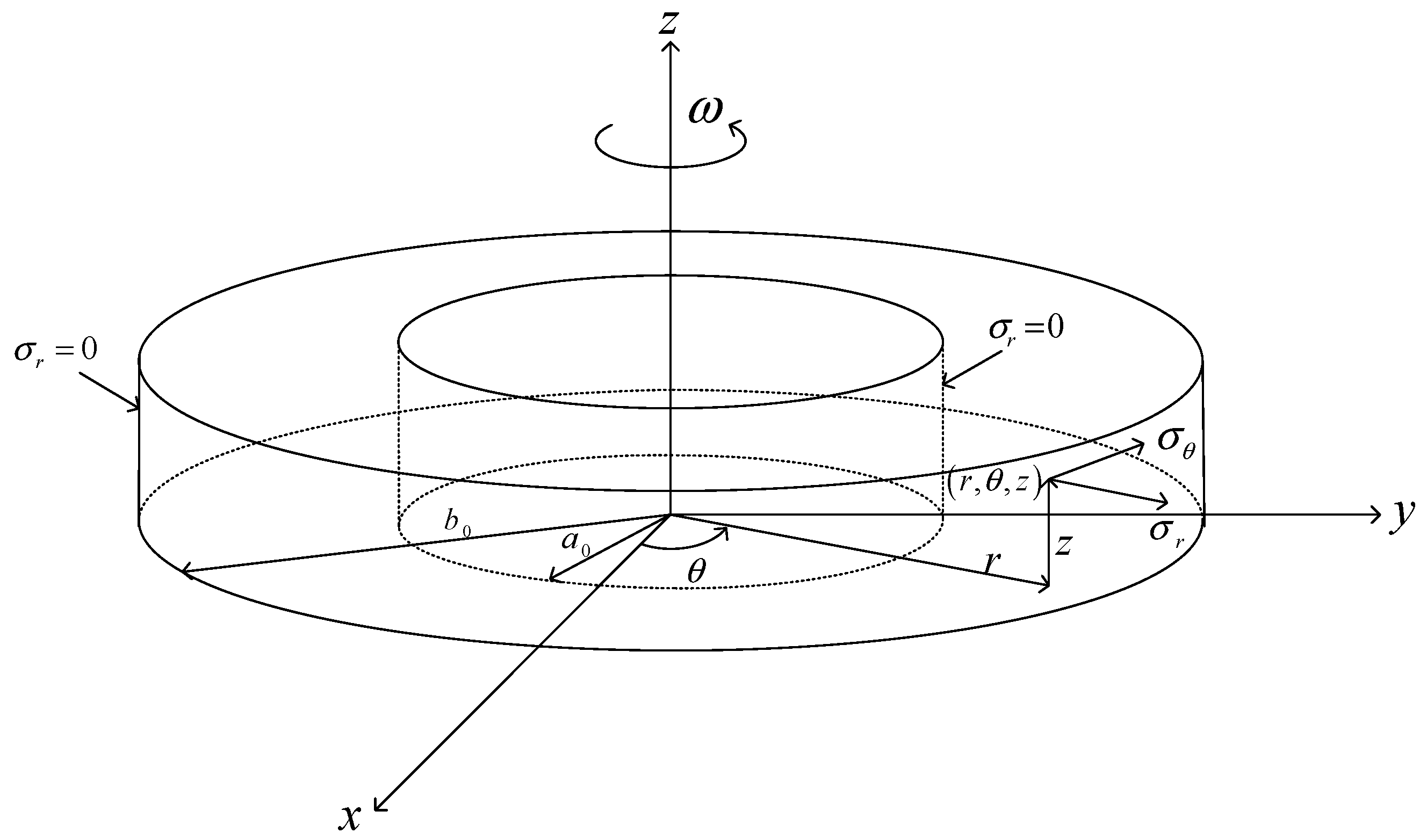
2. Statement of the Problem

A detailed description of the boundary value problem under consideration can be found in many works (see, for example, [11]). The boundary value problem is solved in a cylindrical coordinate system $\left(r,\theta ,z\right)$ whose z axis coincides with the axis of symmetry of a thin annular rotating disk of constant thickness. The assumption of constant thickness is often adopted in theoretical analyses of rotating disks [21,22,23,24,25,26,27,28]. The outer and inner radii of the disk are denoted as $b_0$ and $a_0$, respectively. The angular velocity of the disk is $\omega$. The boundary value problem is illustrated in Figure 1. Strains are small. The disk has no stress at $\omega =0$. The normal stresses in the cylindrical coordinate system, ${\sigma }_r$, ${\sigma }_{\theta }$, and ${\sigma }_z$, are the principal stresses. The solution of the boundary value problem is independent of the polar angle. The state of stress is plane, ${\sigma }_z=0$. The component of the acceleration vector in the circumferential direction is neglected. The stress boundary conditions are:

$${\sigma }_r=0$$

(1)

for $r=a_0$ and $r=b_0$. In general, the disk consists of two regions: elastic and plastic. Hooke’s law connects the elastic strains and stresses. In particular,

$${\epsilon }_r^e=\frac{{\sigma }_r-\nu {\sigma }_{\theta }}{E},{\epsilon }_{\theta }^e=\frac{{\sigma }_{\theta }-\nu {\sigma }_r}{E},{\epsilon }_z^e=-\frac{\nu \left({\sigma }_r+{\sigma }_{\theta }\right)}{E}.$$

(2)

Here, $\nu$ is Poisson’s ratio and E is Young’s modulus, ε_r is the radial strain, ε_θ is the circumferential strain, and ε_z is the axial strain. The superscript e denotes the elastic part of the strain and will denote the elastic part of the strain rate. The orthotropic yield criterion proposed in reference [14] and its associated flow rule are adopted in the plastic region. It is assumed that the principal axes of anisotropy coincide with coordinate curves of the cylindrical coordinate system. Under plane stress conditions, the yield criterion adopted reads $\left(G+H\right){\sigma }_r^2+\left(F+H\right){\sigma }_{\theta }^2-2H{\sigma }_r{\sigma }_{\theta }=1$ where G, H, and F are anisotropic constants. It is convenient to rewrite this criterion as:

$${\sigma }_r^2+\frac{{\sigma }_{\theta }^2}{{\eta }_1^2}-\frac{\eta {\sigma }_r{\sigma }_{\theta }}{{\eta }_1}={\sigma }_0^2$$

(3)

where

$$\eta =\frac{2H}{\sqrt{\left(G+H\right)\left(H+F\right)}},{\eta }_1=\frac{\sqrt{G+H}}{\sqrt{H+F}},⤢{\eta }_2=\frac{2F}{\left(H+F\right)\sqrt{4-{\eta }^2}},{\sigma }_0=\frac{1}{G+H}.$$

(4)

The yield criterion (Equation (3)) reduces to the von Mises yield criterion at $F=G=H$. In this case, ${\sigma }_0$ is the tensile yield stress. Let ${\dot{\epsilon }}_r^p$, ${\dot{\epsilon }}_{\theta }^p$, and ${\dot{\epsilon }}_z^p$ be the plastic strain rates. In the case under consideration, the associated flow rule can be written as [29]:

$${\dot{\epsilon }}_r^p=\lambda \left({\sigma }_r-\frac{\eta }{2{\eta }_1}{\sigma }_{\theta }\right),{\dot{\epsilon }}_{\theta }^p=\frac{\lambda }{{\eta }_1}\left(\frac{{\sigma }_{\theta }}{{\eta }_1}-\frac{\eta }{2}{\sigma }_r\right),{\dot{\epsilon }}_z^p=-\lambda \left[\left(1-\frac{\eta }{2{\eta }_1}\right){\sigma }_r+\left(\frac{1}{{\eta }_1}-\frac{\eta }{2}\right)\frac{{\sigma }_{\theta }}{{\eta }_1}\right]$$

(5)

where $\lambda$ is a non-negative multiplier. The superimposed dot denotes the time derivative at fixed r and the superscript p denotes the plastic part of the strain rate and will denote the plastic part of the strain. The total strains and strain rates in the plastic region are:

$$\begin{array}{l}{\epsilon }_r^{}={\epsilon }_r^e+{\epsilon }_r^p,{\epsilon }_{\theta }^{}={\epsilon }_{\theta }^e+{\epsilon }_{\theta }^p,{\epsilon }_z^{}={\epsilon }_z^e+{\epsilon }_z^p,\\ {\dot{\epsilon }}_r^{}={\dot{\epsilon }}_r^e+{\dot{\epsilon }}_r^p,{\dot{\epsilon }}_{\theta }^{}={\dot{\epsilon }}_{\theta }^e+{\dot{\epsilon }}_{\theta }^p,{\dot{\epsilon }}_z^{}={\dot{\epsilon }}_z^e+{\dot{\epsilon }}_z^p.\end{array}$$

(6)

The equilibrium equation is of the form:

$$\frac{\partial {\sigma }_r}{\partial r}+\frac{{\sigma }_r-{\sigma }_{\theta }}{r}=-\varsigma {\omega }^{2}r.$$

(7)

Here, $\varsigma$ is the mass density of the material.

The boundary value problem is classified by the following dimensionless quantities:

$$\rho =\frac{r}{b_0},\Omega =\frac{\varsigma {\omega }^2{b}_0^2}{{\sigma }_0},a=\frac{a_0}{b_0},k=\frac{{\sigma }_0}{E}.$$

(8)

Since the material model is rate-independent, the time derivative can be replaced with the derivative with respect to $\Omega$. The derivatives of strain components with respect to $\Omega$ are denoted as:

$$\begin{array}{l}{\xi }_r=\frac{\partial {\epsilon }_r}{\partial \Omega },{\xi }_{\theta }=\frac{\partial {\epsilon }_{\theta }}{\partial \Omega },{\xi }_z=\frac{\partial {\epsilon }_z}{\partial \Omega },\\ {\xi }_r^e=\frac{\partial {\epsilon }_r^e}{\partial \Omega },{\xi }_{\theta }^e=\frac{\partial {\epsilon }_{\theta }^e}{\partial \Omega },{\xi }_z^e=\frac{\partial {\epsilon }_z^e}{\partial \Omega },\\ {\xi }_r^p=\frac{\partial {\epsilon }_r^p}{\partial \Omega },{\xi }_{\theta }^p=\frac{\partial {\epsilon }_{\theta }^p}{\partial \Omega },{\xi }_z^p=\frac{\partial {\epsilon }_z^p}{\partial \Omega }.\end{array}$$

(9)

Then, the equation of strain rate compatibility is equivalent to:

$$\rho \frac{\partial {\xi }_{\theta }}{\partial \rho }={\xi }_r-{\xi }_{\theta }.$$

(10)

Using Equation (8), Equation (7) can be rewritten as:

$$\frac{\partial {\sigma }_r}{{\sigma }_0\partial \rho }+\frac{{\sigma }_r-{\sigma }_{\theta }}{{\sigma }_0\rho }=-\Omega \rho .$$

(11)

3. Solution at Loading

3.1. Purely Elastic Solution

The general purely elastic solution for a rotating disk is given, for example, in [3]. Using Equation (8), the solution satisfying the boundary condition (Equation (1)) at $\rho =1$ is represented as:

$$\begin{array}{l}\frac{{\sigma }_r}{{\sigma }_0}=B\left(\frac{1}{{\rho }^2}-1\right)+\frac{\Omega \left(3+\nu \right)}{8}\left(1-{\rho }^2\right),\\ \frac{{\sigma }_{\theta }}{{\sigma }_0}=-B\left(\frac{1}{{\rho }^2}+1\right)+\frac{\Omega \left(1+3\nu \right)}{8}\left(\frac{3+\nu }{1+3\nu }-{\rho }^2\right),\\ \frac{{\epsilon }_r}{k}=\frac{8B\left[1+\nu -\left(1-\nu \right){\rho }^2\right]+\Omega \left(1-\nu \right)\left[3+\nu -3\left(1+\nu \right){\rho }^2\right]{\rho }^2}{8{\rho }^2},\\ \frac{{\epsilon }_{\theta }}{k}=\frac{-8B\left[1+\nu +\left(1-\nu \right){\rho }^2\right]+\Omega \left(1-\nu \right)\left[3+\nu -\left(1+\nu \right){\rho }^2\right]{\rho }^2}{8{\rho }^2},\\ \frac{{\epsilon }_z}{k}=\frac{\nu }{4}\left\{8B-\Omega \left[3+\nu -2\left(1+\nu \right){\rho }^2\right]\right\}.\end{array}$$

(12)

Here, B is a constant of integration. Using the boundary condition (Equation (1)) at $\rho =a$, it is possible to find that:

$$B=-\frac{\Omega \left(3+\nu \right)a^2}{8}.$$

(13)

Eliminating B in Equation (12) by means of Equation (13) provides the solution for the stresses and strains in the purely elastic disk. Let ${\Omega }_e$ be the value of $\Omega$ at which the plastic region starts to develop from the surface $\rho =a$. Substituting the values of ${\sigma }_r$ and ${\sigma }_{\theta }$ at $\rho =a$ into the yield condition Equation (3) and using Equation (4) yields:

$${\Omega }_e=\frac{4{\eta }_1}{3+\nu +a^2\left(1-\nu \right)}.$$

(14)

In what follows, it is assumed that $\Omega >{\Omega }_e$.

The solution (Equation (12)) is valid in the elastic region of the elastic/plastic disk. However, Equation (13) is not valid in this case because one of the boundary conditions in Equation (1) should be replaced with the condition that the radial and circumferential stresses are continuous across the elastic/plastic boundary.

3.2. Elastic/Plastic Stress Solution

The elastic/plastic stress solution is available [30]. For completeness, this solution is outlined below. The yield condition (Equation (3)) is satisfied by the following substitution:

$${\sigma }_r/{\sigma }_0=2\cos \psi /\sqrt{4-{\eta }^2},{\sigma }_{\theta }/{\sigma }_0=\left(\eta \cos \psi /\sqrt{4-{\eta }^2}+\sin \psi \right){\eta }_1$$

(15)

where $\psi$ is a new function of $\rho$ and $\Omega$. Substituting Equation (15) into Equation (11) and using Equation (4) leads to:

$$\frac{2\sin \psi }{\sqrt{4-{\eta }^2}}\frac{\partial \psi }{\partial \rho }+\frac{\left({\eta }_2\cos \psi -{\eta }_1\sin \psi \right)}{\rho }=\Omega \rho .$$

(16)

The boundary condition to this equation is determined from the boundary condition (Equation (1)) at $\rho =a$ and Equation (15) as:

$$\psi =\frac{\pi }{2}$$

(17)

for $\rho =a$. It has been taken into account here that ${\sigma }_{\theta }>0$ at $\rho =a$. Let ${\rho }_c$ be the dimensionless radius of the elastic/plastic boundary. The value of $\psi$ at $\rho ={\rho }_c$ is denoted by ${\psi }_c$. The continuity of the radial and circumferential stresses across the elastic/plastic boundary, together with Equations (12) and (15), leads to:

$$\begin{array}{l}B\left(\frac{1}{{\rho }_c^2}-1\right)+\frac{\Omega \left(3+\nu \right)}{8}\left(1-{\rho }_c^2\right)=2\cos {\psi }_c/\sqrt{4-{\eta }^2},\\ -B\left(\frac{1}{{\rho }_c^2}+1\right)+\frac{\Omega \left(1+3\nu \right)}{8}\left(\frac{3+\nu }{1+3\nu }-{\rho }_c^2\right)=\left(\eta \cos {\psi }_c/\sqrt{4-{\eta }^2}+\sin {\psi }_c\right){\eta }_1.\end{array}$$

(18)

Eliminating B between these equations yields:

$$\begin{array}{l}\frac{2\cos {\psi }_c}{\sqrt{4-{\eta }^2}}+\frac{\left(\eta \cos {\psi }_c/\sqrt{4-{\eta }^2}+\sin {\psi }_c\right)\left(1-{\rho }_c^2\right){\eta }_1}{\left(1+{\rho }_c^2\right)}\\ -\frac{\Omega \left(1-{\rho }_c^2\right)}{8}\left[\frac{\left(1+3\nu \right)}{\left(1+{\rho }_c^2\right)}\left(\frac{3+\nu }{1+3\nu }-{\rho }_c^2\right)+3+\nu \right]=0.\end{array}$$

(19)

For a given value of $\Omega$, Equation (19) and the solution of Equation (16) supply the system of equations for ${\rho }_c$ and ${\psi }_c$. Then, B can be determined from Equation (18). The stress distribution in the elastic region, ${\rho }_c\le \rho \le 1$, follows from Equation (12). The stress distribution in the plastic region, $a\le \rho \le {\rho }_c$, is readily determined from Equation (15) and the solution of Equation (16). The latter is in parametric form with $\psi$ being the parameter. The plastic region occupies the entire disk when ${\rho }_c=1$. Let $\Omega {}_p$ be the corresponding value of $\Omega$. This value can be found numerically using the dependence of ${\rho }_c$ on $\Omega$ known from Equation (19) and the solution of Equation (16). In particular, it is seen from Equation (19) that ${\psi }_c=\pi /2$ at ${\rho }_c=1$. This condition and Equation (17) allow the value of ${\Omega }_p$ and a constant of integration to be determined from the solution of Equation (16).

3.3. Elastic/Plastic Strain Solution

Eliminating B in Equation (12) by means of the solution of Equations (18) and (19) supplies the strain solution in the elastic region as follows in terms of $\Omega$ and $\rho$. Replacing the plastic strain rates in Equation (5) with the corresponding quantities introduced in Equation (9) and eliminating $\lambda$ between the resulting equations leads to:

$${\xi }_r^p={\xi }_{\theta }^p\frac{\left(2{\eta }_1{\sigma }_r-\eta {\sigma }_{\theta }\right){\eta }_1}{\left(2{\sigma }_{\theta }-\eta {\eta }_1{\sigma }_r\right)},{\xi }_z^p={\xi }_{\theta }^p\frac{\left[\left(2{\eta }_1-\eta \right){\eta }_1{\sigma }_r+\left(2-\eta {\eta }_1\right){\sigma }_{\theta }\right]}{\left(\eta {\eta }_1{\sigma }_r-2{\sigma }_{\theta }\right)}.$$

The stresses in these equations can be expressed in terms of $\psi$ by means of Equation (15). Then,

$${\xi }_r^p={\xi }_{\theta }^p\frac{\left(\sqrt{4-{\eta }^2}\cos \psi -\eta \sin \psi \right){\eta }_1}{2\sin \psi },{\xi }_z^p=-{\xi }_{\theta }^p\frac{\left[{\eta }_1\sqrt{4-{\eta }^2}\cos \psi +\left(2-\eta {\eta }_1\right)\sin \psi \right]}{2\sin \psi }.$$

(20)

The elastic portion of the strain components in the plastic region is determined from Equations (2), (8) and (15) as:

$$\begin{array}{l}\frac{{\epsilon }_r^e}{k}=\frac{\left(2-\eta {\eta }_1\nu \right)\cos \psi }{\sqrt{4-{\eta }^2}}-{\eta }_1\nu \sin \psi ,\frac{{\epsilon }_{\theta }^e}{k}=\frac{\left(\eta {\eta }_1-2\nu \right)\cos \psi }{\sqrt{4-{\eta }^2}}+{\eta }_1\sin \psi ,\\ \frac{{\epsilon }_z^e}{k}=\frac{\nu \left(\eta {\eta }_1+2\right)\cos \psi }{\sqrt{4-{\eta }^2}}+\nu {\eta }_1\sin \psi .\end{array}$$

(21)

Differentiating these expressions with respect to $\Omega$ and using Equation (9) yields:

$$\begin{array}{l}\frac{{\xi }_r^e}{k}=-\left[\frac{\left(2-\eta {\eta }_1\nu \right)\sin \psi }{\sqrt{4-{\eta }^2}}+{\eta }_1\nu \cos \psi \right]\frac{\partial \psi }{\partial \Omega },\frac{{\xi }_{\theta }^e}{k}=\left[{\eta }_1\cos \psi -\frac{\left(\eta {\eta }_1-2\nu \right)\sin \psi }{\sqrt{4-{\eta }^2}}\right]\frac{\partial \psi }{\partial \Omega },\\ \frac{{\xi }_z^e}{k}=\nu \left[{\eta }_1\cos \psi -\frac{\left(\eta {\eta }_1+2\right)\sin \psi }{\sqrt{4-{\eta }^2}}\right]\frac{\partial \psi }{\partial \Omega }.\end{array}$$

(22)

Taking into account Equation (6), Equation (10) can be rewritten as $\rho \partial {\xi }_{\theta }/\partial \rho ={\xi }_r^p+{\xi }_r^e-{\xi }_{\theta }^p-{\xi }_{\theta }^e$. Eliminating ${\xi }_r^p$ in this equation by means of Equation (20) results in:

$$\rho \frac{\partial {\xi }_{\theta }}{\partial \rho }=\frac{\left[{\eta }_1\sqrt{4-{\eta }^2}\cos \psi -\left(\eta {\eta }_1+2\right)\sin \psi \right]}{2\sin \psi }{\xi }_{\theta }^p+{\xi }_r^e-{\xi }_{\theta }^e.$$

This equation and Equation (6) combine to give the following equation for ${\xi }_{\theta }$:

$$\rho \frac{\partial {\xi }_{\theta }}{\partial \rho }=\frac{\left[{\eta }_1\sqrt{4-{\eta }^2}\cos \psi -\left(\eta {\eta }_1+2\right)\sin \psi \right]}{2\sin \psi }{\xi }_{\theta }^{}+\frac{{\eta }_1\left[\eta \sin \psi -\sqrt{4-{\eta }^2}\cos \psi \right]}{2\sin \psi }{\xi }_r^e-{\xi }_{\theta }^e$$

(23)

where ${\xi }_r^e$ and ${\xi }_{\theta }^e$ should be eliminated by means of Equation (22). It is therefore evident that Equation (23) is a linear ordinary differential equation. In order to solve this equation, it is necessary to express the derivative $\partial \psi /\partial \Omega$ involved in Equation (22) in terms of $\psi$ or/and $\rho$. Following the method proposed in [8], Equation (16) is differentiated with respect to $\Omega$. Then,

$$\frac{2\sin \psi }{\sqrt{4-{\eta }^2}}\frac{\partial \chi }{\partial \rho }+\left(\frac{2\cos \psi }{\sqrt{4-{\eta }^2}}\frac{\partial \psi }{\partial \rho }+\frac{{\eta }_2\sin \psi +{\eta }_1\cos \psi }{\rho }\right)\chi -\rho =0$$

(24)

where $\chi =\partial \psi /\partial \Omega$. Using Equation (16), the derivative $\partial \psi /\partial \rho$ involved in Equation (24) can be expressed in terms of $\psi$ and $\rho$. Then, Equation (24) becomes:

$$\frac{2\sin \psi }{\sqrt{4-{\eta }^2}}\frac{\partial \chi }{\partial \rho }+\left\{\frac{{\eta }_2\sin \psi +{\eta }_1\cos \psi }{\rho }+2\cos \psi \left[\Omega \rho -\frac{\left({\eta }_2\cos \psi -{\eta }_1\sin \psi \right)}{2\rho \sin \psi }\right]\right\}\chi -\rho =0.$$

(25)

It follows from the boundary condition (Equation (17)) that $\partial \psi /\partial \Omega =0$ at $\rho =a$. Therefore,

$$\chi =0$$

(26)

at $\rho =a$. This is the boundary condition to Equation (25), which is a linear ordinary differential equation for $\chi$. This equation should be solved numerically. Once $\chi$ has been found from Equation (25), it is possible to determine ${\xi }_r^e$ and ${\xi }_{\theta }^e$ involved in Equation (23) as functions of $\psi$ and $\rho$ by means of Equation (22). Having $\psi$ as a function of $\rho$ due to the solution of Equation (16), it is possible to represent the coefficients of Equation (23) as functions of $\rho$. Then, this ordinary differential equation can be solved numerically with no difficulty. The boundary condition to Equation (23) follows from the continuity of the circumferential strain rate and, therefore, ${\xi }_{\theta }$ across the elastic/plastic boundary $\rho ={\rho }_c$. The value of ${\xi }_{\theta }$ on the elastic side of this boundary is determined from Equation (12) as:

$$\frac{{\xi }_c}{k}=\frac{\left(1-\nu \right)\left[3+\nu -\left(1+\nu \right){\rho }_c^2\right]}{8}-\frac{\left[1+\nu +\left(1-\nu \right){\rho }_c^2\right]}{{\rho }_c^2}\frac{dB}{d\Omega }.$$

(27)

Then, the boundary condition to Equation (23) is

$${\xi }_{\theta }={\xi }_c$$

(28)

for $\rho ={\rho }_c$. Once the solution of Equation (23) has been found, the total circumferential strain in the plastic region is determined by integration of ${\xi }_{\theta }$ with respect to $\Omega$ at a given point $\rho ={\rho }_t$. The maximum value of $\Omega$ is denoted as ${\Omega }_f$ and the corresponding value of ${\rho }_c$ as ${\rho }_f$. It is assumed that ${\Omega }_f<{\Omega }_p$. It is obvious that $a\le {\rho }_t<{\rho }_f$. The value of $\Omega$ and the value of the circumferential strain on the elastic side of the elastic/plastic boundary at ${\rho }_c={\rho }_t$ are denoted as ${\Omega }_t$ and $E_{\theta }^t$, respectively. Then, it follows from the definition for ${\xi }_{\theta }$ given in Equation (9) that:

$${\epsilon }_{\theta }={\displaystyle \underset{{\Omega }_t}{\overset{{\Omega }_f}{\int }}{\xi }_{\theta }d\Omega }+E_{\theta }^t.$$

(29)

The value of $E_{\theta }^t$ is determined from Equation (12) as:

$$\frac{E_{\theta }^t}{k}=\frac{-8B_t\left[1+\nu +\left(1-\nu \right){\rho }_t^2\right]+{\Omega }_t\left(1-\nu \right)\left[3+\nu -\left(1+\nu \right){\rho }_t^2\right]{\rho }_t^2}{8{\rho }_t^2}.$$

(30)

Here $B_t$ is the value of B at ${\rho }_c={\rho }_t$. This value follows from Equations (18) and (19). Equations (6) and (22) combine to give:

$${\xi }_{\theta }^p={\xi }_{\theta }-k\left[{\eta }_1\cos \psi -\frac{\left(\eta {\eta }_1-2\nu \right)\sin \psi }{\sqrt{4-{\eta }^2}}\right]\chi .$$

(31)

Substituting Equation (31) into Equation (20) leads to:

$$\begin{array}{l}\frac{{\xi }_r^p}{k}=\frac{{\eta }_1}{2}\left\{\frac{{\xi }_{\theta }}{k}-\left[{\eta }_1\cos \psi -\frac{\left(\eta {\eta }_1-2\nu \right)\sin \psi }{\sqrt{4-{\eta }^2}}\right]\chi \right\}\frac{\left(\sqrt{4-{\eta }^2}\cos \psi -\eta \sin \psi \right)}{\sin \psi },\\ \frac{{\xi }_z^p}{k}=-\frac{1}{2}\left\{\frac{{\xi }_{\theta }}{k}-\left[{\eta }_1\cos \psi -\frac{\left(\eta {\eta }_1-2\nu \right)\sin \psi }{\sqrt{4-{\eta }^2}}\right]\chi \right\}\frac{\left[{\eta }_1\sqrt{4-{\eta }^2}\cos \psi +\left(2-\eta {\eta }_1\right)\sin \psi \right]}{\sin \psi }.\end{array}$$

(32)

Hence,

$$\frac{{\epsilon }_r^p}{k}={\displaystyle \underset{{\Omega }_t}{\overset{{\Omega }_f}{\int }}\frac{{\xi }_r^p}{k}}d\Omega ,\frac{{\epsilon }_z^p}{k}={\displaystyle \underset{{\Omega }_t}{\overset{{\Omega }_f}{\int }}\frac{{\xi }_z^p}{k}}d\Omega .$$

(33)

Here, the integrands are known functions of $\Omega$. In particular, ${\xi }_r^p$ and ${\xi }_z^p$ are first eliminated by means of Equation (32). Then, the solutions of Equations (16), (23) and (25) are used to represent $\psi$, ${\xi }_{\theta }$, and $\chi$, respectively, as functions of $\Omega$ at any value of $\rho ={\rho }_t$. Therefore, the integrals involved in Equation (33) can be evaluated numerically. The total radial and axial strains in the plastic zone are found by means of Equation (6) where the plastic parts are given by Equation (33) and the elastic parts by Equation (21).

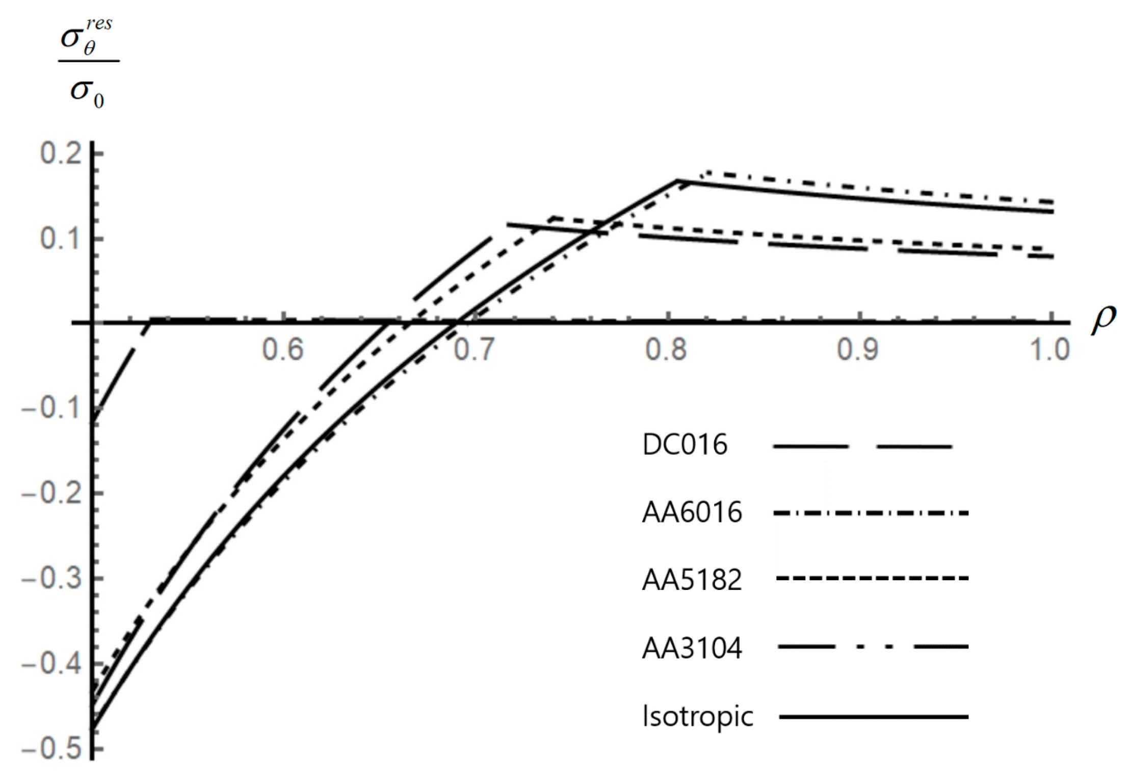
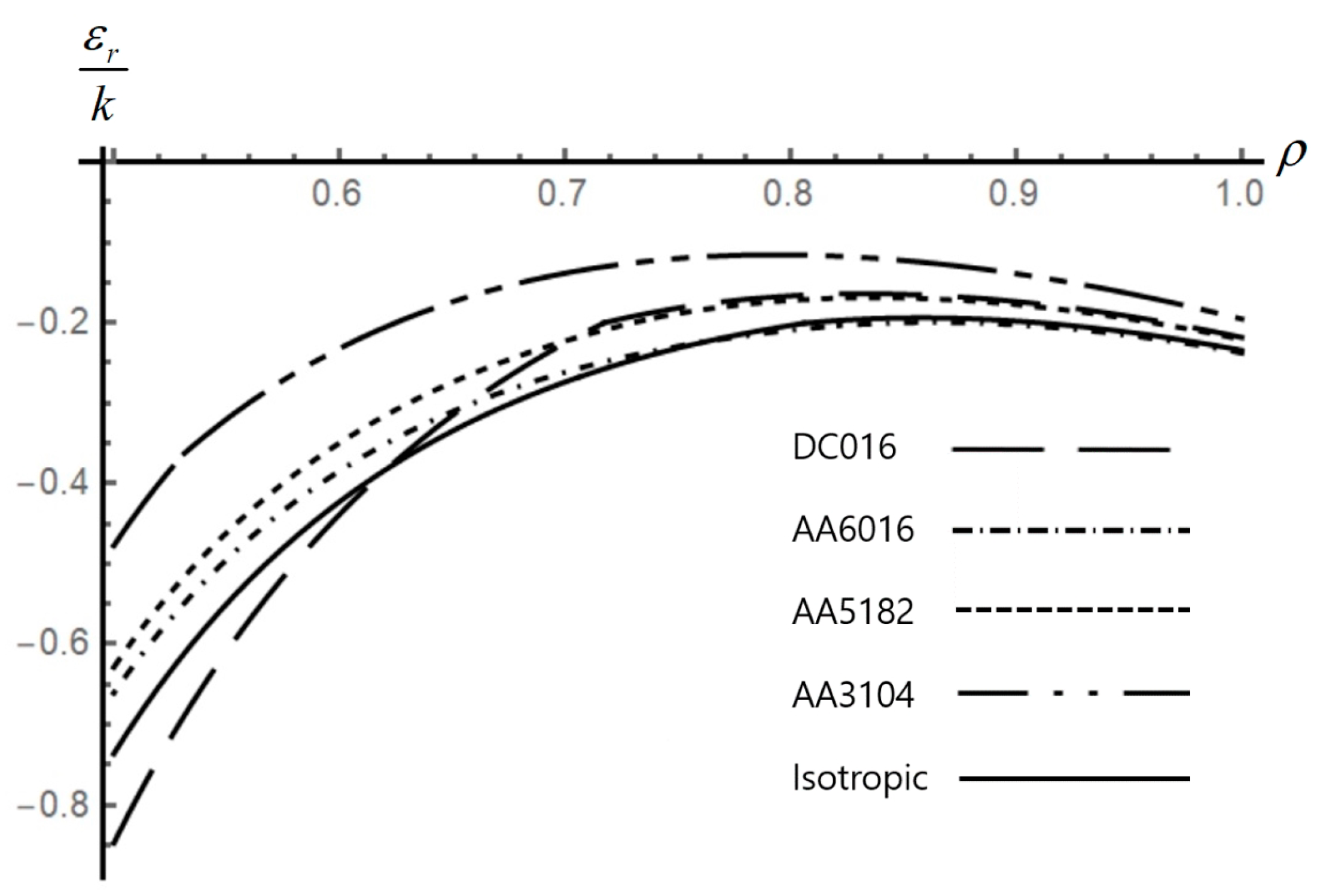
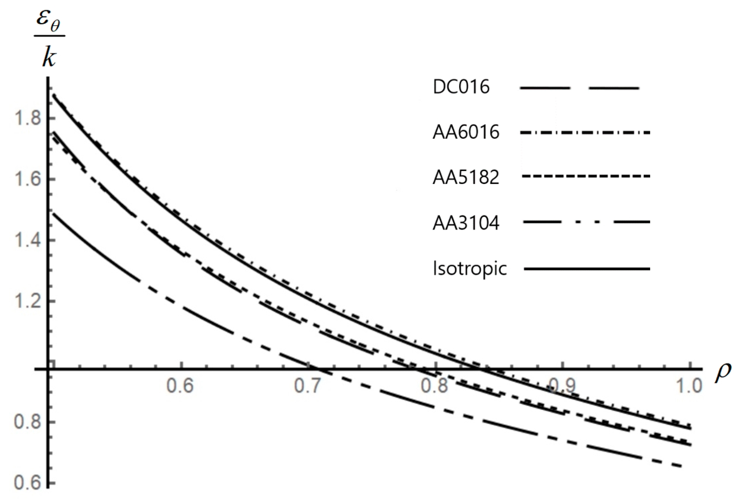
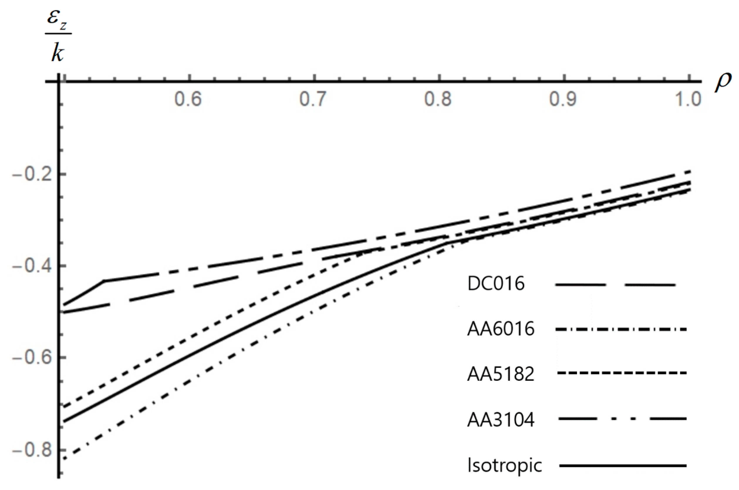
4. Distribution of Residual Stresses and Strains

It is assumed that unloading is purely elastic (i.e., the distribution of residual stresses found by means of Hooke’s law for the increments of stresses does not violate the yield criterion in the range $a\le \rho \le 1$). This assumption should be verified a posteriori. The residual stresses are determined as:

$${\sigma }_r^{res}={\sigma }_r^f+\Delta {\sigma }_r,{\sigma }_{\theta }^{res}={\sigma }_{\theta }^f+\Delta {\sigma }_{\theta }.$$

(34)

Here, ${\sigma }_r^f$ and ${\sigma }_{\theta }^f$ are the radial and circumferential stresses, respectively, at the end of loading. These stresses were found in the previous section. $\Delta {\sigma }_r$ and $\Delta {\sigma }_{\theta }$ are the increments of the radial and circumferential stresses, respectively, in the course of the process of unloading. Analogously, the residual strains are determined as:

$${\epsilon }_r^{res}={\epsilon }_r^f+\Delta {\epsilon }_r,{\epsilon }_{\theta }^{res}={\epsilon }_{\theta }^f+\Delta {\epsilon }_{\theta },{\epsilon }_z^{res}={\epsilon }_z^f+\Delta {\epsilon }_z.$$

(35)

Here, ${\epsilon }_r^f$, ${\epsilon }_{\theta }^f$, and ${\epsilon }_z^f$ are the total radial, circumferential, and axial strains, respectively, at the end of loading. These strains were found in the previous section. $\Delta {\epsilon }_r$, $\Delta {\epsilon }_{\theta }$, and $\Delta {\epsilon }_z$ are the increments of the radial, circumferential, and axial strains, respectively, in the course of the process of unloading. Since the process of unloading is assumed to be purely elastic, the increments of the strains are related by Hooke’s law to the increments of the stresses:

$$\Delta {\epsilon }_r^e=\frac{\Delta {\sigma }_r-\nu \Delta {\sigma }_{\theta }}{E},\Delta {\epsilon }_{\theta }^e=\frac{\Delta {\sigma }_{\theta }-\nu \Delta {\sigma }_r}{E},\Delta {\epsilon }_z^e=-\frac{\nu \left(\Delta {\sigma }_r+\Delta {\sigma }_{\theta }\right)}{E}.$$

(36)

Therefore, the solution (Equations (12) and (13)) in which $\Omega$ should be replaced with $-{\Omega }_f$ is valid. As a result,

$$\begin{array}{l}\frac{\Delta {\sigma }_r}{{\sigma }_0}=B_f\left(\frac{1}{{\rho }^2}-1\right)-\frac{{\Omega }_f\left(3+\nu \right)}{8}\left(1-{\rho }^2\right),\\ \frac{\Delta {\sigma }_{\theta }}{{\sigma }_0}=-B_f\left(\frac{1}{{\rho }^2}+1\right)-\frac{{\Omega }_f\left(1+3\nu \right)}{8}\left(\frac{3+\nu }{1+3\nu }-{\rho }^2\right),\\ \frac{\Delta {\epsilon }_r}{k}=\frac{8B_f\left[1+\nu -\left(1-\nu \right){\rho }^2\right]-{\Omega }_f\left(1-\nu \right)\left[3+\nu -3\left(1+\nu \right){\rho }^2\right]{\rho }^2}{8{\rho }^2},\\ \frac{\Delta {\epsilon }_{\theta }}{k}=\frac{-8B_f\left[1+\nu +\left(1-\nu \right){\rho }^2\right]-{\Omega }_f\left(1-\nu \right)\left[3+\nu -\left(1+\nu \right){\rho }^2\right]{\rho }^2}{8{\rho }^2},\\ \frac{\Delta {\epsilon }_z}{k}=\frac{\nu }{4}\left\{8B_f+{\Omega }_f\left[3+\nu -2\left(1+\nu \right){\rho }^2\right]\right\}\end{array}$$

(37)

where

$$B_f=\frac{{\Omega }_f\left(3+\nu \right)a^2}{8}.$$

(38)

Substituting the solution found in the previous section together with Equations (37) and (38) into Equation (35) yields the distribution of residual stresses and strains. It follows from Equation (3) that the yield criterion is not violated after unloading if:

$${\left(\frac{{\sigma }_r^{res}}{{\sigma }_0}\right)}^2+{\left(\frac{{\sigma }_{\theta }^{res}}{{\sigma }_0{\eta }_1}\right)}^2-\frac{\eta }{{\eta }_1}\left(\frac{{\sigma }_r^{res}}{{\sigma }_0}\right)\left(\frac{{\sigma }_{\theta }^{res}}{{\sigma }_0}\right)-1\le 0.$$

(39)

Since the distribution of the residual stresses has been found, this inequality can be verified with no difficulty.

5. Illustrative Example

Equations (16), (23) and (24) were solved numerically for several materials whose anisotropic coefficients, given in [31,32], are shown in

Table 1. Anisotropic coefficients of several materials.

Material	F/(G + H)	H/(G + H)
DC06	0.243	0.703
AA6016	0.587	0.410
AA5182	0.498	0.419
AA3014	0.239	0.301
Isotropic	0.5	0.5

. It is assumed that $\nu =0.3$ in all cases. The value of k introduced in Equation (8) is immaterial. In particular, assume that the solution for a disk of given geometry and physical properties has been found. Then, simple scaling of this solution supplies the solutions for similar disks of material with the same Poisson’s ratio and anisotropic coefficients but any value of k. The numerical solution is illustrated for an $a=0.5$ disk at ${\Omega }_f=1.7$. The distribution of stresses is depicted in Figure 2 and Figure 3 and residual stresses in Figure 4 and Figure 5. The associated total and plastic strain fields are shown in Figure 6, Figure 7, Figure 8, Figure 9, Figure 10 and Figure 11. The variation of the residual strains with $\rho$ is depicted in Figure 12, Figure 13 and Figure 14. The solution for the residual stresses was used in conjunction with Equation (39) to verify that the process of unloading is purely elastic. It is evident from Figure 3 that the effect of plastic anisotropy on the radius of the elastic plastic boundary is very significant and, as a result, so is the effect of plastic anisotropy on the distribution of stresses, strains, residual stresses, and residual strains. On the other hand, the yield loci for the anisotropic parameters considered are depicted in Figure 15. It is seen from this figure that the yield loci for the materials considered are not very different (except for the yield locus for AA3104). This sensitivity of solutions to the yield locus requires very accurate numerical methods for calculating stress and strain fields. Therefore, it is of interest to compare the present solution and a finite difference solution. The present solution involves fewer approximations than finite difference solutions because the derivative $\partial \psi /\partial \Omega$ is found from Equation (24) without any discretization with respect to $\Omega$ (i.e., with respect to time). Therefore, it is natural to assume that the present solution is more accurate. In [10], several finite difference solutions were found for an $a=3/7$ disk assuming that ${\rho }_f=5/7$ (in our nomenclature). Using the anisotropic constants adopted in [10], the distribution of the circumferential strain was determined using the method proposed in the present paper. A comparison of the magnitude of circumferential strain at $\rho =a$ and ${\rho }_f=5/7$ (in our nomenclature) predicted by the new method and that found in [10] is presented in

Table 2. Comparison of the total circumferential strain at $\rho =a$ and ${\rho }_f=5/7$ found by the two methods.

F/(G + H)	H/(G + H)	${\mathit{\epsilon }}_{\mathit{\theta },\mathit{F}\mathit{D}\mathit{M}}$	${\mathit{\epsilon }}_{\mathit{\theta },\mathit{N}}$	$\mathbf{\Delta }$ (%)
0.452	0.681	0.00088	0.00134	26.3
0.421	0.615	0.0014	0.0019	34.4
0.283	0.634	0.00178	0.00212	16.0
0.811	0.454	0.0025	0.0036	30.6
0.5	0.5	0.0019	0.0022	13.6

. It can be seen from this table that the accuracy of the finite difference solution may be insufficient for practical applications. In particular, $\Delta$ shown in Table 2 is defined as:

$$\Delta =\frac{\left|{\epsilon }_{\theta ,FDM}-{\epsilon }_{\theta ,N}\right|}{{\epsilon }_{\theta ,N}}\times 100\%$$

where ${\epsilon }_{\theta ,FDM}$ is the total circumferential strain at $\rho =a$ and ${\rho }_f=5/7$ found in [10] and ${\epsilon }_{\theta ,N}$ is the total circumferential strain at $\rho =a$ and ${\rho }_f=5/7$ found in the present paper.

6. Conclusions

A semi-analytic solution for the stresses and strains within a rotating elastic/plastic polar orthotropic annular disk was found under plane stress. The range of validity of plane stress solutions was determined in [33] by comparing such solutions with 3-D finite element solutions. The distribution of residual stresses and strains was determined as well. The constitutive equations consist of Hooke’s law, the orthotropic yield criterion proposed in [14], and the associated flow rule. Therefore, the equations to be solved involve the strain rate tensor. This greatly adds to the difficulties of the solution as compared with the constitutive equations that relate the stresses to the strains (or allow for the strains to be immediately found by integrating relations between strain rate components). In order to facilitate numerical solution, the method developed in [11] was adopted. As a result, it is only necessary to use numerical methods for solving ordinary differential equations and to evaluate ordinary integrals, even though the solution depends on two independent variables—$\Omega$ and $\rho$.

It is seen from Equations (12), (21), (22), (32) and (33) that the parameter k introduced in Equation (8) is immaterial in the sense that scaling of any strain solution for a disk of given radius, Poisson’s ratio, and anisotropic parameters provides the solutions for similar disks of material with the same Poisson’s ratio and anisotropic parameters but any value of k.

It is known that numerical codes should be verified before their use in applications [34,35,36]. The present solution is useful for this purpose since ordinary differential equations can be solved numerically with a very high accuracy with no difficulty. In particular, comparison with the finite difference solution proposed in [10] was made. It was shown that the accuracy of the finite difference solution for the total circumferential strain at the inner radius of the disk may be insufficient (Table 2).

The solution found is for a rate-independent model of plasticity. However, in many cases, solutions for rate-dependent plasticity are required [37]. Moreover, disks of varying thickness and disks made of functionally graded materials are widely used in industry [38]. The general approach used in the present paper can be extended to at least some of these cases. This will be the subject of a subsequent investigation.

References

1. Tahani, M.; Nosier, A.; Zebarjad, S.M. Deformation and stress analysis of circumferentially fiber-reinforced composite disks. Int. J. Solids Struct. 2005, 42, 2741–2754. [Google Scholar] [CrossRef]
2. Zare, H.R.; Darijani, H. Strengthening and design of the linear hardening thick-walled cylinders using the new method of rotational autofrettage. Int. J. Mech. Sci. 2017, 124–125, 1–8. [Google Scholar] [CrossRef]
3. Timoshenko, S.P.; Goodier, J.N. Theory of Elasticity, 3rd ed.; McGraw-Hill: New York, NY, USA, 1970. [Google Scholar]
4. Arnold, S.M.; Saleeb, A.F.; Al-Zoubi, N.R. Deformation and life analysis of composite flywheel disk systems. Compos. Part B Eng. 2002, 33, 433–459. [Google Scholar] [CrossRef]
5. Yildirim, V. Numerical/analytical solution to the elastic response of arbitrarily functionally graded polar orthotropic rotating discs. J. Braz. Soc. Mech. Sci. Eng. 2018, 40, 320. [Google Scholar] [CrossRef]
6. Eraslan, A.N. Inelastic deformations of rotating variable thickness solid disks by Tresca and von Mises criteria. Int. J. Comput. Eng. Sci. 2002, 3, 89–101. [Google Scholar] [CrossRef]
7. Hojjati, M.H.; Hassani, A. Theoretical and numerical analyses of rotating disks of non-uniform thickness and density. Int. J. Press. Vessel. Pip. 2008, 85, 694–700. [Google Scholar] [CrossRef]
8. Alexandrova, N.; Alexandrov, S.; Vila Real, P. Displacement field and strain distribution in a rotating annular disk. Mech. Based Des. Struct. 2004, 32, 441–457. [Google Scholar] [CrossRef]
9. Argeso, H. Analytical solutions to variable thickness and variable material property rotating disks for a new three-parameter variation function. Mech. Based Des. Struct. 2012, 40, 133–152. [Google Scholar] [CrossRef]
10. Alexandrova, N.N.; Real, P.M.M.V. Effect of anisotropy on stress-strain field in thin rotating disks. Thin Walled Struct. 2006, 44, 897–903. [Google Scholar] [CrossRef]
11. Lomakin, E.; Alexandrov, S.; Jeng, Y.-R. Stress and strain fields in rotating elastic/plastic annular discs. Arch. Appl. Mech. 2016, 86, 235–244. [Google Scholar] [CrossRef]
12. Alexandrov, S.; Chung, K.; Jeong, W. Stress and strain fields in rotating elastic/plastic annular disks of pressure-dependent material. Mech. Based Des. Struct. 2018, 46, 318–332. [Google Scholar] [CrossRef]
13. Prime, M.B. Amplified effect of mild plastic anisotropy on residual stress and strain anisotropy. Int. J. Solids Struct. 2017, 118, 70–77. [Google Scholar] [CrossRef]
14. Hill, R. The Mathematical Theory of Plasticity; Clarendon Press: Oxford, UK, 1950. [Google Scholar]
15. Singh, S.B.; Ray, S. Modeling the anisotropy and creep in orthotropic aluminum-silicon carbide composite rotating disc. Mech. Mater. 2002, 34, 363–372. [Google Scholar] [CrossRef]
16. Alexandrova, N.N.; Real, P.M.M.V. Singularities in a solution to a rotating orthotropic disk with temperature gradient. Meccanica 2006, 41, 197–205. [Google Scholar] [CrossRef]
17. Ari-Gur, J.; Stavsky, Y. On rotating polar-orthotropic circular disks. Int. J. Solids Struct. 1981, 17, 57–67. [Google Scholar] [CrossRef]
18. Liang, D.S.; Wang, H.J.; Chen, L.W. Vibration and stability of rotating polar orthotropic annular disks subjected to a stationary concentrated transverse load. J. Sound Vib. 2002, 250, 795–811. [Google Scholar] [CrossRef]
19. Koo, K.N. Vibration analysis and critical speeds of polar orthotropic annular disks in rotation. Compos. Struct. 2006, 76, 67–72. [Google Scholar] [CrossRef]
20. Peng, X.-L.; Li, X.-F. Elastic analysis of rotating functionally graded polar orthotropic disks. Int. J. Mech. Sci. 2012, 60, 84–91. [Google Scholar] [CrossRef]
21. Bert, C.W.; Paul, T.K. Failure analysis of rotating disks. Int. J. Solids Struct. 1995, 32, 1307–1318. [Google Scholar] [CrossRef]
22. You, L.H.; Zhang, J.J. Elastic-plastic stresses in a rotating solid disk. Int. J. Mech. Sci. 1999, 41, 269–282. [Google Scholar] [CrossRef]
23. Yahnioglu, N.; Akbarov, S.D. Stability loss analyses of the elastic and viscoplastic composite rotating thick circular plate in the framework of the three-dimensional linearized theory of stability. Int. J. Mech. Sci. 2002, 44, 1225–1244. [Google Scholar] [CrossRef]
24. Portnov, G.G.; Ochan, M.Y.; Bakis, C.E. Critical state of imbalanced rotating anisotropic disks with small radial and shear moduli. Int. J. Solids Struct. 2003, 40, 5219–5227. [Google Scholar] [CrossRef]
25. Çallıoğlu, H.; Topcu, M.; Tarakcılar, A.R. Elastic-plastic stress analysis of an orthotropic rotating disc. Int. J. Mech. Sci. 2006, 48, 985–990. [Google Scholar] [CrossRef]
26. Rees, D.W.A. A theory for swaging of discs and lugs. Meccanica 2011, 46, 1213–1237. [Google Scholar] [CrossRef]
27. Daghigh, V.; Daghigh, H.; Loghman, A.; Simoneau, A. Time-dependent creep analysis of rotating ferritic steel disk using Taylor series and Prandtl-Reuss relation. Int. J. Mech. Sci. 2013, 77, 40–46. [Google Scholar] [CrossRef]
28. Aleksandrova, N. Exact deformation analysis of a solid rotating elastic-perfectly plastic disk. Int. J. Mech. Sci. 2014, 88, 55–60. [Google Scholar] [CrossRef]
29. Alexandrov, S. Elastic/Plastic Disks under Plane Stress Conditions; Springer: New York, NY, USA, 2015. [Google Scholar]
30. Alexandrova, N.N.; Alexandrov, S. Elastic-plastic stress distribution in a plastically anisotropic rotating disk. J. Appl. Mech. 2004, 71, 427–429. [Google Scholar] [CrossRef]
31. Bouvier, S.; Teodosiu, C.; Haddadi, H.; Tabacaru, V. Anisotropic work-hardening behavior of structural steels and aluminium alloys at large strains. J. Phys. IV France 2003, 105, 215. [Google Scholar] [CrossRef]
32. Wu, P.D.; Jain, M.; Savoie, J.; MacEwen, S.R.; Tugcu, P.; Neale, K.W. Evaluation of anisotropic yield functions for aluminum sheets. Int. J. Plast. 2003, 19, 121–138. [Google Scholar] [CrossRef]
33. Kammal, S.M.; Dixit, U.S.; Roy, A.; Liu, Q.; Silberschmidt, V.V. Comparison of plane-stress, generalized-plane-strain and 3D FEM elastic-plastic analyses of thick-walled cylinders subjected to radial thermal gradient. Int. J. Mech. Sci. 2017, 131–132, 744–752. [Google Scholar] [CrossRef]
34. Roberts, S.M.; Hall, F.R.; Bael, A.V.; Hartley, P.; Pillinger, I.; Sturgess, C.E.N.; Houtte, P.V.; Aernoudt, E. Benchmark tests for 3-D, elasto-plastic, finite-element codes for the modelling of metal forming processes. J. Mater. Process. Technol. 1992, 34, 61–68. [Google Scholar] [CrossRef]
35. Becker, A.A.; Hyde, T.H.; Sun, W.; Andersson, P. Benchmarks for finite element analysis of creep continuum damage mechanics. Comp. Mater. Sci. 2002, 25, 34–41. [Google Scholar] [CrossRef]
36. Helsing, J.; Jonsson, A. On the accuracy of benchmark tables and graphical results in the applied mechanics literature. J. Appl. Mech. 2002, 69, 88–90. [Google Scholar] [CrossRef]
37. Zharfi, H.; EkhteraeiToussi, H. Time dependent creep analysis in thick FGM rotating disk with two-dimensional patterns of heterogeneity. Int. J. Mech. Sci. 2018, 140, 351–360. [Google Scholar] [CrossRef]
38. Yildirim, V. A parametric study on the centrifugal force-induced stress and displacements in power-law graded hyperbolic discs. Lat. Am. J. Solids Strut. 2018, 15, e34. [Google Scholar]
Figure 1. Schematic diagram of a rotating annular disk.
Symmetry 10 00420 g001
Figure 2. Effect of anisotropic properties on the distribution of the radial stress in an a = 0.5 disk.
Symmetry 10 00420 g002
Figure 3. Effect of anisotropic properties on the distribution of the circumferential stress in an a = 0.5 disk.
Symmetry 10 00420 g003
Figure 4. Effect of anisotropic properties on the distribution of the residual radial stress in an a = 0.5 disk.
Symmetry 10 00420 g004
Figure 5. Effect of anisotropic properties on the distribution of the residual circumferential stress in an a = 0.5 disk.
Symmetry 10 00420 g005
Figure 6. Effect of anisotropic properties on the distribution of the radial strain in an a = 0.5 disk.
Symmetry 10 00420 g006
Figure 7. Effect of anisotropic properties on the distribution of the circumferential strain in an a = 0.5 disk.
Symmetry 10 00420 g007
Figure 8. Effect of anisotropic properties on the distribution of the axial strain in an a = 0.5 disk.
Symmetry 10 00420 g008
Figure 9. Effect of anisotropic properties on the distribution of the radial plastic strain in an a = 0.5 disk.
Symmetry 10 00420 g009
Figure 10. Effect of anisotropic properties on the distribution of the circumferential plastic strain in an a = 0.5 disk.
Symmetry 10 00420 g010
Figure 11. Effect of anisotropic properties on the distribution of the axial plastic strain in an a = 0.5 disk.
Symmetry 10 00420 g011
Figure 12. Effect of anisotropic properties on the distribution of the residual radial strain in an a = 0.5 disk.
Symmetry 10 00420 g012
Figure 13. Effect of anisotropic properties on the distribution of the residual circumferential strain in an a = 0.5 disk.
Symmetry 10 00420 g013
Figure 14. Effect of anisotropic properties on the distribution of the residual axial strain in an a = 0.5 disk.
Symmetry 10 00420 g014
Figure 15. Yield loci for several materials.
Symmetry 10 00420 g015