Two Types of Single Valued Neutrosophic Covering Rough Sets and an Application to Decision Making

Abstract

In this paper, to combine single valued neutrosophic sets (SVNSs) with covering-based rough sets, we propose two types of single valued neutrosophic (SVN) covering rough set models. Furthermore, a corresponding application to the problem of decision making is presented. Firstly, the notion of SVN $\beta$-covering approximation space is proposed, and some concepts and properties in it are investigated. Secondly, based on SVN $\beta$-covering approximation spaces, two types of SVN covering rough set models are proposed. Then, some properties and the matrix representations of the newly defined SVN covering approximation operators are investigated. Finally, we propose a novel method to decision making (DM) problems based on one of the SVN covering rough set models. Moreover, the proposed DM method is compared with other methods in an example.

1. Introduction

Rough set theory, as a a tool to deal with various types of data in data mining, was proposed by Pawlak [1,2] in 1982. Since then, rough set theory has been extended to generalized rough sets based on other notions such as binary relations, neighborhood systems and coverings.

Covering-based rough sets [3,4,5] were proposed to deal with the type of covering data. In application, they have been applied to knowledge reduction [6,7], decision rule synthesis [8,9], and other fields [10,11,12]. In theory, covering-based rough set theory has been connected with matroid theory [13,14,15,16], lattice theory [17,18] and fuzzy set theory [19,20,21,22].

Zadeh’s fuzzy set theory [23] addresses the problem of how to understand and manipulate imperfect knowledge. It has been used in various applications [24,25,26,27]. Recent investigations have attracted more attention on combining covering-based rough set and fuzzy set theories. There are many fuzzy covering rough set models proposed by researchers, such as Ma [28] and Yang et al. [20].

Wang et al. [29] presented single valued neutrosophic sets (SVNSs) which can be regarded as an extension of IFSs [30]. Neutrosophic sets and rough sets both can deal with partial and uncertain information. Therefore, it is necessary to combine them. Recently, Mondal and Pramanik [31] presented the concept of rough neutrosophic set. Yang et al. [32] presented a SVN rough set model based on SVN relations. However, SVNSs and covering-based rough sets have not been combined up to now. In this paper, we present two types of SVN covering rough set models. This new combination is a bridge, linking SVNSs and covering-based rough sets.

As we know, the multiple criteria decision making (MCDM) is an important tool to deal with more complicated problems in our real world [33,34]. There are many MCDM methods presented based on different problems or theories. For example, Liu et al. [35] dealt with the challenges of many criteria in the MCDM problem and decision makers with heterogeneous risk preferences. Watróbski et al. [36] proposed a framework for selecting suitable MCDA methods for a particular decision situation. Faizi et al. [37,38] presented an extension of the MCDM method based on hesitant fuzzy theory. Recently, many researchers have studied decision making (DM) problems by rough set models [39,40,41,42]. For example, Zhan et al. [39] applied a type of soft rough model to DM problems. Yang et al. [32] presented a method for DM problems under a type of SVN rough set model. By investigation, we have observed that no one has applied SVN covering rough set models to DM problems. Therefore, we construct the covering SVN decision information systems according to the characterizations of DM problems. Then, we present a novel method to DM problems under one of the SVN covering rough set models. Moreover, the proposed decision making method is compared with other methods, which were presented by Yang et al. [32], Liu [43] and Ye [44].

The rest of this paper is organized as follows. Section 2 reviews some fundamental definitions about covering-based rough sets and SVNSs. In Section 3, some notions and properties in SVN $\beta$-covering approximation space are studied. In Section 4, we present two types of SVN covering rough set models, based on the SVN $\beta$-neighborhoods and the $\beta$-neighborhoods. In Section 5, some new matrices and matrix operations are presented. Based on this, the matrix representations of the SVN approximation operators are shown. In Section 6, a novel method to decision making (DM) problems under one of the SVN covering rough set models is proposed. Moreover, the proposed DM method is compared with other methods. This paper is concluded and further work is indicated in Section 7.

2. Basic Definitions

Suppose U is a nonempty and finite set called universe.

Definition 1

(Covering [45,46]). Let U be a universe and $\mathit{C}$ a family of subsets of U. If none of subsets in $\mathit{C}$ is empty and $\bigcup \mathit{C}=U$, then $\mathit{C}$ is called a covering of U.

The pair $(U,\mathbf{C})$ is called a covering approximation space.

Definition 2

(Single valued neutrosophic set [29]). Let U be a nonempty fixed set. A single valued neutrosophic set (SVNS) A in U is defined as an object of the following form:

$$A=\{\langle x,T_A(x),I_A(x),F_A(x)\rangle :x\in U\},$$

where $T_A(x):U\to [0,1]$ is a truth-membership function, $I_A(x):U\to [0,1]$ is an indeterminacy-membership function and $F_A(x):U\to [0,1]$ is a falsity-membership function for any $x\in U$. They satisfy $0\le T_A(x)+I_A(x)+F_A(x)\le 3$ for all $x\in U$. The family of all single valued neutrosophic sets in U is denoted by $SVN(U)$. For convenience, a SVN number is represented by $\alpha =\langle a,b,c\rangle$, where $a,b,c\in [0,1]$ and $a+b+c\le 3$.

Specially, for two SVN numbers $\alpha =\langle a,b,c\rangle$ and $\beta =\langle d,e,f\rangle$, $\alpha \le \beta \iff a\le d$, $b\ge e$ and $c\ge f$. Some operations on $SVN(U)$ are listed as follows [29,32]: for any $A,B\in SVN(U)$,

(1)

$A\subseteq B$ iff $T_A(x)\le T_B(x)$, $I_B(x)\le I_A(x)$ and $F_B(x)\le F_A(x)$ for all $x\in U$.

(2)

$A=B$ iff $A\subseteq B$ and $B\subseteq A$.

(3)

$A\cap B=\{\langle x,T_A(x)\wedge T_B(x),I_A(x)\vee I_B(x),F_A(x)\vee F_B(x)\rangle :x\in U\}$.

(4)

$A\cup B=\{\langle x,T_A(x)\vee T_B(x),I_A(x)\wedge I_B(x),F_A(x)\wedge F_B(x)\rangle :x\in U\}$.

(5)

$A^{\prime }=\{\langle x,F_A(x),1-I_A(x),T_A(x)\rangle :x\in U\}$.

(6)

$A\oplus B=\{\langle x,T_A(x)+T_B(x)-T_A(x)·T_B(x),I_A(x)·I_B(x),F_A(x)·F_B(x)\rangle :x\in U\}$.

3. Single Valued Neutrosophic $\beta$-Covering Approximation Space

In this section, we present the notion of SVN $\beta$-covering approximation space. There are two basic concepts in this new approximation space: SVN $\beta$-covering and SVN $\beta$-neighborhood. Then, some of their properties are studied.

Definition 3.

Let U be a universe and $SVN(U)$ be the SVN power set of U. For a SVN number $\beta =\langle a,b,c\rangle$, we call $\widehat{\mathit{C}}=\{C_1,C_2,\cdots ,C_m\}$, with $C_i\in SVN(U)(i=1,2,\dots ,m)$, a SVN β-covering of U, if for all $x\in U$, $C_i\in \widehat{\mathit{C}}$ exists such that $C_i(x)\ge \beta$. We also call $(U,\widehat{\mathit{C}})$ a SVN β-covering approximation space.

Definition 4.

Let $\widehat{\mathit{C}}$ be a SVN β-covering of U and $\widehat{\mathit{C}}=\{C_1,C_2,\dots ,C_m\}$. For any $x\in U$, the SVN β-neighborhood ${\tilde{\mathbb{N}}}_x^{\beta }$ of x induced by $\widehat{\mathit{C}}$ can be defined as:

$${\tilde{\mathbb{N}}}_x^{\beta }=\cap \{C_i\in \widehat{\mathit{C}}:C_i(x)\ge \beta \}.$$

(1)

Note that $C_i(x)$ is a SVN number $\langle T_{C_i}(x),I_{C_i}(x),F_{C_i}(x)\rangle$ in Definitions 3 and 4. Hence, $C_i(x)\ge \beta$ means $T_{C_i}(x)\ge a$, $I_{C_i}(x)\le b$ and $F_{C_i}(x)\le c$ where SVN number $\beta =\langle a,b,c\rangle$.

Remark 1.

Let $\widehat{\mathit{C}}$ be a SVN β-covering of U, $\beta =\langle a,b,c\rangle$ and $\widehat{\mathit{C}}=\{C_1,C_2,\dots ,C_m\}$. For any $x\in U$,

$${\tilde{\mathbb{N}}}_x^{\beta }=\cap \{C_i\in \widehat{\mathit{C}}:T_{C_i}(x)\ge a,I_{C_i}(x)\le b,F_{C_i}(x)\le c\}.$$

(2)

Example 1.

Let $U=\{x_1,x_2,x_3,x_4,x_5\}$, $\widehat{\mathit{C}}=\{C_1,C_2,C_3,C_4\}$ and $\beta =\langle 0.5,0.3,0.8\rangle$. We can see that $\widehat{\mathit{C}}$ is a SVN β-covering of U in

Table 1. The tabular representation of single valued neutrosophic (SVN) β-covering $\widehat{\mathit{C}}$.

$\mathit{U}$	${\mathit{C}}_{\mathbf{1}}$	${\mathit{C}}_{\mathbf{2}}$	${\mathit{C}}_{\mathbf{3}}$	${\mathit{C}}_{\mathbf{4}}$
$x_1$	$\langle 0.7,0.2,0.5\rangle$	$\langle 0.6,0.2,0.4\rangle$	$\langle 0.4,0.1,0.5\rangle$	$\langle 0.1,0.5,0.6\rangle$
$x_2$	$\langle 0.5,0.3,0.2\rangle$	$\langle 0.5,0.2,0.8\rangle$	$\langle 0.4,0.5,0.4\rangle$	$\langle 0.6,0.1,0.7\rangle$
$x_3$	$\langle 0.4,0.5,0.2\rangle$	$\langle 0.2,0.3,0.6\rangle$	$\langle 0.5,0.2,0.4\rangle$	$\langle 0.6,0.3,0.4\rangle$
$x_4$	$\langle 0.6,0.1,0.7\rangle$	$\langle 0.4,0.5,0.7\rangle$	$\langle 0.3,0.6,0.5\rangle$	$\langle 0.5,0.3,0.2\rangle$
$x_5$	$\langle 0.3,0.2,0.6\rangle$	$\langle 0.7,0.3,0.5\rangle$	$\langle 0.6,0.3,0.5\rangle$	$\langle 0.8,0.1,0.2\rangle$

.

Then,

$$\begin{array}{c}{\tilde{\mathbb{N}}}_{x_1}^{\beta }=C_1\cap C_2,{\tilde{\mathbb{N}}}_{x_2}^{\beta }=C_1\cap C_2\cap C_4,{\tilde{\mathbb{N}}}_{x_3}^{\beta }=C_3\cap C_4,{\tilde{\mathbb{N}}}_{x_4}^{\beta }=C_1\cap C_4,{\tilde{\mathbb{N}}}_{x_5}^{\beta }=C_2\cap C_3\cap C_4.\hfill \end{array}$$

Hence, all SVN $\beta$-neighborhoods are shown in

Table 2. The tabular representation of ${\tilde{\mathbb{N}}}_{x_k}^{\beta }$ ($k=1,2,3,4,5$).

${\tilde{\mathbb{N}}}_{{\mathit{x}}_{\mathit{k}}}^{\mathit{\beta }}$	${\mathit{x}}_1$	${\mathit{x}}_2$	${\mathit{x}}_3$	${\mathit{x}}_4$	${\mathit{x}}_5$
${\tilde{\mathbb{N}}}_{x_1}^{\beta }$	$\langle 0.6,0.2,0.5\rangle$	$\langle 0.5,0.3,0.8\rangle$	$\langle 0.2,0.5,0.6\rangle$	$\langle 0.4,0.5,0.7\rangle$	$\langle 0.3,0.3,0.6\rangle$
${\tilde{\mathbb{N}}}_{x_2}^{\beta }$	$\langle 0.1,0.5,0.6\rangle$	$\langle 0.5,0.3,0.8\rangle$	$\langle 0.2,0.5,0.6\rangle$	$\langle 0.4,0.5,0.7\rangle$	$\langle 0.3,0.3,0.6\rangle$
${\tilde{\mathbb{N}}}_{x_3}^{\beta }$	$\langle 0.1,0.5,0.6\rangle$	$\langle 0.4,0.5,0.7\rangle$	$\langle 0.5,0.3,0.4\rangle$	$\langle 0.3,0.6,0.5\rangle$	$\langle 0.6,0.3,0.5\rangle$
${\tilde{\mathbb{N}}}_{x_4}^{\beta }$	$\langle 0.1,0.5,0.6\rangle$	$\langle 0.5,0.3,0.7\rangle$	$\langle 0.4,0.5,0.4\rangle$	$\langle 0.5,0.3,0.7\rangle$	$\langle 0.3,0.2,0.6\rangle$
${\tilde{\mathbb{N}}}_{x_5}^{\beta }$	$\langle 0.1,0.5,0.6\rangle$	$\langle 0.4,0.5,0.8\rangle$	$\langle 0.2,0.3,0.6\rangle$	$\langle 0.3,0.6,0.7\rangle$	$\langle 0.6,0.3,0.5\rangle$

.

In a SVN $\beta$-covering approximation space $(U,\widehat{\mathit{C}})$, we present the following properties of the SVN $\beta$-neighborhood.

Theorem 1.

Let $\widehat{\mathit{C}}$ be a SVN β-covering of U and $\widehat{\mathit{C}}=\{C_1,C_2,\dots ,C_m\}$. Then, the following statements hold:

(1)

${\tilde{\mathbb{N}}}_x^{\beta }(x)\ge \beta$ for each $x\in U$.

(2)

$\forall x,y,z\in U$, if ${\tilde{\mathbb{N}}}_x^{\beta }(y)\ge \beta$, ${\tilde{\mathbb{N}}}_y^{\beta }(z)\ge \beta$, then ${\tilde{\mathbb{N}}}_x^{\beta }(z)\ge \beta$.

(3)

For two SVN numbers ${\beta }_1,{\beta }_2$, if ${\beta }_1\le {\beta }_2\le \beta$, then ${\tilde{\mathbb{N}}}_x^{{\beta }_1}\subseteq {\tilde{\mathbb{N}}}_x^{{\beta }_2}$ for all $x\in U$.

Proof. 

(1)

For any $x\in U$, ${\tilde{\mathbb{N}}}_x^{\beta }(x)=(\bigcap _{C_i(x)\ge \beta }{C}_i)(x)=\underset{C_i(x)\ge \beta }{\bigwedge }{C}_i(x)\ge \beta$.

(2)

Let $I=\{1,2,\cdots ,m\}$. Since ${\tilde{\mathbb{N}}}_x^{\beta }(y)\ge \beta$, for any $i\in I$, if $C_i(x)\ge \beta$, then $C_i(y)\ge \beta$. Since ${\tilde{\mathbb{N}}}_y^{\beta }(z)\ge \beta$, for any $i\in I$, $C_i(z)\ge \beta$ when $C_i(y)\ge \beta$. Then, for any $i\in I$, $C_i(x)\ge \beta$ implies $C_i(z)\ge \beta$. Therefore, ${\tilde{\mathbb{N}}}_x^{\beta }(z)\ge \beta$.

(3)

For all $x\in U$, since ${\beta }_1\le {\beta }_2\le \beta$, $\{C_i\in \widehat{\mathbf{C}}:C_i(x)\ge {\beta }_1\}\supseteq \{C_i\in \widehat{\mathbf{C}}:C_i(x)\ge {\beta }_2\}$. Hence, ${\tilde{\mathbb{N}}}_x^{{\beta }_1}=\cap \{C_i\in \widehat{\mathbf{C}}:C_i(x)\ge {\beta }_1\}\subseteq \cap \{C_i\in \widehat{\mathbf{C}}:C_i(x)\ge {\beta }_2\}={\tilde{\mathbb{N}}}_x^{{\beta }_2}$ for all $x\in U$.

□

Proposition 1.

Let $\widehat{\mathit{C}}$ be a SVN β-covering of U. For any $x,y\in U$, ${\tilde{\mathbb{N}}}_x^{\beta }(y)\ge \beta$ if and only if ${\tilde{\mathbb{N}}}_y^{\beta }\subseteq {\tilde{\mathbb{N}}}_x^{\beta }$.

Proof. 

Suppose the SVN number $\beta =\langle a,b,c\rangle$.

$(\Rightarrow )$: Since ${\tilde{\mathbb{N}}}_x^{\beta }(y)\ge \beta$,

$$T_{{\tilde{\mathbb{N}}}_x^{\beta }}(y)=T_{{\displaystyle \underset{F_{C_i}(x)\le c}{\underset{I_{C_i}(x)\le b}{\bigcap _{T_{C_i}(x)\ge a}}}}{C}_i}(y)={\displaystyle \underset{F_{C_i}(x)\le c}{\underset{I_{C_i}(x)\le b}{\underset{T_{C_i}(x)\ge a}{\bigwedge }}}}{T}_{C_i}(y)\ge a,I_{{\tilde{\mathbb{N}}}_x^{\beta }}(y)=I_{{\displaystyle \underset{F_{C_i}(x)\le b}{\underset{I_{C_i}(x)\le c}{\bigcap _{T_{C_i}(x)\ge a}}}}{C}_i}(y)={\displaystyle \underset{F_{C_i}(x)\le c}{\underset{I_{C_i}(x)\le b}{\underset{T_{C_i}(x)\ge a}{\bigvee }}}}{I}_{C_i}(y)\le b$$

, and

$$F_{{\tilde{\mathbb{N}}}_x^{\beta }}(y)=F_{{\displaystyle \underset{F_{C_i}(x)\le b}{\underset{I_{C_i}(x)\le c}{\bigcap _{T_{C_i}(x)\ge a}}}}{C}_i}(y)={\displaystyle \underset{F_{C_i}(x)\le c}{\underset{I_{C_i}(x)\le b}{\underset{T_{C_i}(x)\ge a}{\bigvee }}}}{F}_{C_i}(y)\le c$$

.

Then,

$$\{C_i\in \widehat{\mathbf{C}}:T_{C_i}(x)\ge a,I_{C_i}(x)\le b,F_{C_i}(x)\le c\}\subseteq \{C_i\in \widehat{\mathbf{C}}:T_{C_i}(y)\ge a,I_{C_i}(y)\le b,F_{C_i}(y)\le c\}$$

.

Therefore, for each $z\in U$,

$$\begin{array}{c}{T}_{{\tilde{\mathbb{N}}}_x^{\beta }}(z)={\displaystyle \underset{F_{C_i}(x)\le c}{\underset{I_{C_i}(x)\le b}{\underset{T_{C_i}(x)\ge a}{\bigwedge }}}}{T}_{C_i}(z)\ge {\displaystyle \underset{F_{C_i}(y)\le c}{\underset{I_{C_i}(y)\le b}{\underset{T_{C_i}(y)\ge a}{\bigwedge }}}}{T}_{C_i}(z)=T_{{\tilde{\mathbb{N}}}_y^{\beta }}(z),\hfill \\ I_{{\tilde{\mathbb{N}}}_x^{\beta }}(z)={\displaystyle \underset{F_{C_i}(x)\le c}{\underset{I_{C_i}(x)\le b}{\underset{T_{C_i}(x)\ge a}{\bigvee }}}}{I}_{C_i}(z)\le {\displaystyle \underset{F_{C_i}(y)\le c}{\underset{I_{C_i}(y)\le b}{\underset{T_{C_i}(y)\ge a}{\bigvee }}}}{I}_{C_i}(z)=I_{{\tilde{\mathbb{N}}}_y^{\beta }}(z),\hfill \\ F_{{\tilde{\mathbb{N}}}_x^{\beta }}(z)={\displaystyle \underset{F_{C_i}(x)\le c}{\underset{I_{C_i}(x)\le b}{\underset{T_{C_i}(x)\ge a}{\bigvee }}}}{F}_{C_i}(z)\le {\displaystyle \underset{F_{C_i}(y)\le c}{\underset{I_{C_i}(y)\le b}{\underset{T_{C_i}(y)\ge a}{\bigvee }}}}{F}_{C_i}(z)=F_{{\tilde{\mathbb{N}}}_y^{\beta }}(z).\hfill \end{array}$$

Hence, ${\tilde{\mathbb{N}}}_y^{\beta }\subseteq {\tilde{\mathbb{N}}}_x^{\beta }$.

$(\Leftarrow )$: For any $x,y\in U$, since ${\tilde{\mathbb{N}}}_y^{\beta }\subseteq {\tilde{\mathbb{N}}}_x^{\beta }$,

$$T_{{\tilde{\mathbb{N}}}_x^{\beta }}(y)\ge T_{{\tilde{\mathbb{N}}}_y^{\beta }}(y)\ge a,I_{{\tilde{\mathbb{N}}}_x^{\beta }}(y)\le I_{{\tilde{\mathbb{N}}}_y^{\beta }}(y)\le b\text{ and }{F}_{{\tilde{\mathbb{N}}}_x^{\beta }}(y)\le F_{{\tilde{N}}_y^{\beta }}(y)\le c$$

.

Therefore, ${\tilde{\mathbb{N}}}_x^{\beta }(y)\ge \beta$. □

The notion of SVN $\beta$-neighborhood in the SVN $\beta$-covering approximation space in the following definition.

Definition 5.

Let $(U,\widehat{\mathit{C}})$ be a SVN β-covering approximation space and $\widehat{\mathit{C}}=\{C_1,C_2,\dots ,C_m\}$. For each $x\in U$, we define the β-neighborhood ${\overline{\mathbb{N}}}_x^{\beta }$ of x as:

$${\overline{\mathbb{N}}}_x^{\beta }=\{y\in U:{\tilde{\mathbb{N}}}_x^{\beta }(y)\ge \beta \}.$$

(3)

Note that ${\tilde{\mathbb{N}}}_x^{\beta }(y)$ is a SVN number $\langle T_{{\tilde{\mathbb{N}}}_x^{\beta }}(y),I_{{\tilde{\mathbb{N}}}_x^{\beta }}(y),F_{{\tilde{\mathbb{N}}}_x^{\beta }}(y)\rangle$ in Definition 5.

Remark 2.

Let $\widehat{\mathit{C}}$ be a SVN β-covering of U, $\beta =\langle a,b,c\rangle$ and $\widehat{\mathit{C}}=\{C_1,C_2,\dots ,C_m\}$. For each $x\in U$,

$${\overline{\mathbb{N}}}_x^{\beta }=\{y\in U:T_{{\tilde{\mathbb{N}}}_x^{\beta }}(y)\ge a,I_{{\tilde{\mathbb{N}}}_x^{\beta }}(y)\le b,F_{{\tilde{\mathbb{N}}}_x^{\beta }}(y)\le c\}.$$

(4)

Example 2

(Continued from Example 1). Let $\beta =\langle 0.5,0.3,0.8\rangle$, then we have

$$\begin{array}{c}{\overline{\mathbb{N}}}_{x_1}^{\beta }=\{x_1,x_2\},{\overline{\mathbb{N}}}_{x_2}^{\beta }=\{x_2\},{\overline{\mathbb{N}}}_{x_3}^{\beta }=\{x_3,x_5\},{\overline{\mathbb{N}}}_{x_4}^{\beta }=\{x_2,x_4\},{\overline{\mathbb{N}}}_{x_5}^{\beta }=\{x_5\}.\hfill \end{array}$$

Some properties of the $\beta$-neighborhood in a SVN $\beta$-covering of U are presented in Theorem 2 and Proposition 2.

Theorem 2.

Let $\widehat{\mathit{C}}$ be a SVN β-covering of U and $\widehat{\mathit{C}}=\{C_1,C_2,\dots ,C_m\}$. Then, the following statements hold:

(1)

$x\in {\overline{\mathbb{N}}}_x^{\beta }$ for each $x\in U$.

(2)

$\forall x,y,z\in U$, if $x\in {\overline{\mathbb{N}}}_y^{\beta }$, $y\in {\overline{\mathbb{N}}}_z^{\beta }$, then $x\in {\overline{\mathbb{N}}}_z^{\beta }$.

Proof. 

(1)

According to Theorem 1 and Definition 5, it is straightforward.

(2)

For any $x,y,z\in U$, $x\in {\overline{\mathbb{N}}}_y^{\beta }\iff {\tilde{\mathbb{N}}}_y^{\beta }(x)\ge \beta \iff {\tilde{\mathbb{N}}}_x^{\beta }\subseteq {\tilde{\mathbb{N}}}_y^{\beta }$, and $y\in {\overline{\mathbb{N}}}_z^{\beta }\iff {\tilde{\mathbb{N}}}_z^{\beta }(y)\ge \beta \iff {\tilde{\mathbb{N}}}_y^{\beta }\subseteq {\tilde{\mathbb{N}}}_z^{\beta }$. Hence, ${\tilde{\mathbb{N}}}_x^{\beta }\subseteq {\tilde{\mathbb{N}}}_z^{\beta }$. By Proposition 1, we have ${\tilde{\mathbb{N}}}_z^{\beta }(x)\ge \beta$, i.e., $x\in {\overline{\mathbb{N}}}_z^{\beta }$.

□

Proposition 2.

Let $\widehat{\mathit{C}}$ be a SVN β-covering of U and $\widehat{\mathit{C}}=\{C_1,C_2,\dots ,C_m\}$. Then, for all $x\in U$, $x\in {\overline{\mathbb{N}}}_y^{\beta }$ if and only if ${\overline{\mathbb{N}}}_x^{\beta }\subseteq {\overline{\mathbb{N}}}_y^{\beta }$.

Proof. 

$(\Rightarrow )$: For any $z\in {\overline{\mathbb{N}}}_x^{\beta }$, we know ${\tilde{\mathbb{N}}}_x^{\beta }(z)\ge \beta$. Since $x\in {\overline{\mathbb{N}}}_y^{\beta }$, ${\tilde{\mathbb{N}}}_y^{\beta }(x)\ge \beta$. According to $(2)$ in Theorem 1, we have ${\tilde{\mathbb{N}}}_y^{\beta }(z)\ge \beta$. Hence, $z\in {\overline{\mathbb{N}}}_y^{\beta }$. Therefore, ${\overline{\mathbb{N}}}_x^{\beta }\subseteq {\overline{\mathbb{N}}}_y^{\beta }$.

$(\Leftarrow )$: According to $(1)$ in Theorem 2, $x\in {\overline{\mathbb{N}}}_x^{\beta }$ for all $x\in U$. Since ${\overline{\mathbb{N}}}_x^{\beta }\subseteq {\overline{\mathbb{N}}}_y^{\beta }$, $x\in {\overline{\mathbb{N}}}_y^{\beta }$. □

The relationship between SVN $\beta$-neighborhoods and $\beta$-neighborhoods is presented in the following proposition.

Proposition 3.

Let $\widehat{\mathit{C}}$ be a SVN β-covering of U. For any $x,y\in U$, ${\tilde{\mathbb{N}}}_x^{\beta }\subseteq {\tilde{\mathbb{N}}}_y^{\beta }$ if and only if ${\overline{\mathbb{N}}}_x^{\beta }\subseteq {\overline{\mathbb{N}}}_y^{\beta }$.

Proof. 

According to Propositions 1 and 2, it is straightforward. □

4. Two Types of Single Valued Neutrosophic Covering Rough Set Models

In this section, we propose two types of SVN covering rough set models on basis of the SVN $\beta$-neighborhoods and the $\beta$-neighborhoods, respectively. Then, we investigate the properties of the defined lower and upper approximation operators.

Definition 6.

Let $(U,\widehat{\mathit{C}})$ be a SVN β-covering approximation space. For each $A\in SVN(U)$ where $A=\{\langle x,T_A(x),$ $I_A(x),F_A(x)\rangle :x\in U\}$, we define the single valued neutrosophic (SVN) covering upper approximation $\tilde{\mathbb{C}}(A)$ and lower approximation $\underset{\sim }{\mathbb{C}}(A)$ of A as:

$$\begin{array}{c}{\displaystyle \tilde{\mathbb{C}}(A)=\{\langle x,{\vee }_{y\in U}[T_{{\tilde{\mathbb{N}}}_x^{\beta }}(y)\wedge T_A(y)],{\vee }_{y\in U}[I_{{\tilde{\mathbb{N}}}_x^{\beta }}(y)\wedge I_A(y)],{\wedge }_{y\in U}[F_{{\tilde{\mathbb{N}}}_x^{\beta }}(y)\vee F_A(y)]\rangle :x\in U\},}\hfill \\ {\displaystyle \underset{\sim }{\mathbb{C}}(A)=\{\langle x,{\wedge }_{y\in U}[F_{{\tilde{\mathbb{N}}}_x^{\beta }}(y)\vee T_A(y)],{\wedge }_{y\in U}[(1-I_{{\tilde{\mathbb{N}}}_x^{\beta }}(y))\vee I_A(y)],{\vee }_{y\in U}[T_{{\tilde{\mathbb{N}}}_x^{\beta }}(y)\wedge F_A(y)]\rangle :x\in U\}.}\hfill \end{array}$$

(5)

If $\tilde{\mathbb{C}}(A)\ne \underset{\sim }{\mathbb{C}}(A)$, then A is called the first type of SVN covering rough set.

Example 3

(Continued from Example 1). Let $\beta =\langle 0.5,0.3,0.8\rangle$, $A=\frac{(0.6,0.3,0.5)}{x_1}+\frac{(0.4,0.5,0.1)}{x_2}+\frac{(0.3,0.2,0.6)}{x_3}+\frac{(0.5,0.3,0.4)}{x_4}+\frac{(0.7,0.2,0.3)}{x_5}$. Then,

$$\begin{array}{c}\tilde{\mathbb{C}}(A)=\{\langle x_1,0.6,0.3,0.5\rangle ,\langle x_2,0.4,0.3,0.6\rangle ,\langle x_3,0.6,0.5,0.5\rangle ,\langle x_4,0.5,0.3,0.6\rangle ,\langle x_5,0.6,0.5,0.5\rangle \},\hfill \\ \underset{\sim }{\mathbb{C}}(A)=\{\langle x_1,0.6,0.5,0.5\rangle ,\langle x_2,0.6,0.5,0.4\rangle ,\langle x_3,0.4,0.4,0.5\rangle ,\langle x_4,0.4,0.5,0.4\rangle ,\langle x_5,0.6,0.4,0.3\rangle \}.\hfill \end{array}$$

Some basic properties of the SVN covering upper and lower approximation operators are proposed in the following proposition.

Proposition 4.

Let $\widehat{\mathit{C}}$ be a SVN β-covering of U. Then, the SVN covering upper and lower approximation operators in Definition 6 satisfy the following properties: for all $A,B\in SVN(U)$,

(1)

$\tilde{\mathbb{C}}(A^{\prime })={(\underset{\sim }{\mathbb{C}}(A))}^{\prime }$, $\underset{\sim }{\mathbb{C}}(A^{\prime })={(\tilde{\mathbb{C}}(A))}^{\prime }$.

(2)

If $A\subseteq B$, then $\underset{\sim }{\mathbb{C}}(A)\subseteq \underset{\sim }{\mathbb{C}}(B)$, $\tilde{\mathbb{C}}(A)\subseteq \tilde{\mathbb{C}}(B)$.

(3)

$\underset{\sim }{\mathbb{C}}(A\bigcap B)={\displaystyle \underset{\sim }{\mathbb{C}}(A)\bigcap \underset{\sim }{\mathbb{C}}}(B)$, $\tilde{\mathbb{C}}(A\bigcup B)=\tilde{\mathbb{C}}(A)\bigcup \tilde{\mathbb{C}}(B)$.

(4)

$\underset{\sim }{\mathbb{C}}(A\bigcup B)\supseteq \underset{\sim }{\mathbb{C}}(A)\bigcup \underset{\sim }{\mathbb{C}}(B)$, $\tilde{\mathbb{C}}(A\bigcap B)\subseteq \tilde{\mathbb{C}}(A)\bigcap \tilde{\mathbb{C}}(B)$.

Proof. 

(1)

$$\begin{array}{cc}\tilde{\mathbb{C}}(A^{\prime })\hfill & =\{\langle x,{\vee }_{y\in U}[T_{{\tilde{\mathbb{N}}}_x^{\beta }}(y)\wedge T_{A^{\prime }}(y)],{\vee }_{y\in U}[I_{{\tilde{\mathbb{N}}}_x^{\beta }}(y)\wedge I_{A^{\prime }}(y)],{\wedge }_{y\in U}[F_{{\tilde{\mathbb{N}}}_x^{\beta }}(y)\vee F_{A^{\prime }}(y)]\rangle :x\in U\}\hfill \\ & =\{\langle x,{\vee }_{y\in U}[T_{{\tilde{\mathbb{N}}}_x^{\beta }}(y)\wedge F_A(y)],{\vee }_{y\in U}[I_{{\tilde{\mathbb{N}}}_x^{\beta }}(y)\wedge (1-I_A(y))],{\wedge }_{y\in U}[F_{{\tilde{\mathbb{N}}}_x^{\beta }}(y)\vee T_A(y)]\rangle :x\in U\}\hfill \\ & ={(\underset{\sim }{\mathbb{C}}(A))}^{\prime }.\hfill \end{array}$$

If we replace A by $A^{\prime }$ in this proof, we can also prove $\underset{\sim }{\mathbb{C}}(A^{\prime })={(\tilde{\mathbb{C}}(A))}^{\prime }$.

(2)

Since $A\subseteq B$, so $T_A(x)\le T_B(x)$, $I_B(x)\le I_A(x)$ and $F_B(x)\le F_A(x)$ for all $x\in U$. Therefore,

$$\begin{array}{c}{T}_{\underset{\sim }{\mathbb{C}}(A)}(x)={\wedge }_{y\in U}[F_{{\tilde{\mathbb{N}}}_x^{\beta }}(y)\vee T_A(y)]\le {\wedge }_{y\in U}[F_{{\tilde{\mathbb{N}}}_x^{\beta }}(y)\vee T_B(y)]=T_{\underset{\sim }{\mathbb{C}}(B)}(x),\hfill \\ I_{\underset{\sim }{\mathbb{C}}(A)}(x)={\wedge }_{y\in U}[(1-I_{{\tilde{\mathbb{N}}}_x^{\beta }}(y))\vee I_A(y)]\ge {\wedge }_{y\in U}[(1-I_{{\tilde{\mathbb{N}}}_x^{\beta }}(y))\vee I_B(y)]=I_{\underset{\sim }{\mathbb{C}}(B)}(x),\hfill \\ F_{\underset{\sim }{\mathbb{C}}(A)}(x)={\vee }_{y\in U}[T_{{\tilde{\mathbb{N}}}_x^{\beta }}(y)\wedge F_A(y)]\ge {\vee }_{y\in U}[T_{{\tilde{\mathbb{N}}}_x^{\beta }}(y)\wedge F_B(y)]=F_{\underset{\sim }{\mathbb{C}}(B)}(x).\hfill \end{array}$$

Hence, $\underset{\sim }{\mathbb{C}}(A)\subseteq \underset{\sim }{\mathbb{C}}(B)$. In the same way, there is $\tilde{\mathbb{C}}(A)\subseteq \tilde{\mathbb{C}}(B)$.

(3)

$$\begin{array}{cc}& \underset{\sim }{\mathbb{C}}(A\bigcap B)\hfill \\ =\hfill & \{\langle x,{\wedge }_{y\in U}[F_{{\tilde{\mathbb{N}}}_x^{\beta }}(y)\vee T_{A\bigcap B}(y)],{\wedge }_{y\in U}[(1-I_{{\tilde{\mathbb{N}}}_x^{\beta }}(y))\vee I_{A\bigcap B}(y)],{\vee }_{y\in U}[T_{{\tilde{\mathbb{N}}}_x^{\beta }}(y)\wedge F_{A\bigcap B}(y)]\rangle :x\in U\}\hfill \\ =\hfill & \{\langle x,{\wedge }_{y\in U}[F_{{\tilde{\mathbb{N}}}_x^{\beta }}(y)\vee (T_A(y)\wedge T_B(y))],{\wedge }_{y\in U}[(1-I_{{\tilde{\mathbb{N}}}_x^{\beta }}(y))\vee (I_A(y)\vee I_B(y))],{\vee }_{y\in U}[T_{{\tilde{\mathbb{N}}}_x^{\beta }}(y)\wedge (F_A(y)\hfill \\ & \vee F_B(y))]\rangle :x\in U\}\hfill \\ =\hfill & \{\langle x,{\wedge }_{y\in U}[(F_{{\tilde{\mathbb{N}}}_x^{\beta }}(y)\vee T_A(y))\wedge (F_{{\tilde{\mathbb{N}}}_x^{\beta }}(y)\vee T_B(y))],{\wedge }_{y\in U}[((1-I_{{\tilde{\mathbb{N}}}_x^{\beta }}(y))\vee I_A(y))\vee (1-I_{{\tilde{\mathbb{N}}}_x^{\beta }}(y))\vee \hfill \\ & I_B(y))],{\vee }_{y\in U}[(T_{{\tilde{\mathbb{N}}}_x^{\beta }}(y)\wedge F_A(y))\vee (T_{{\tilde{\mathbb{N}}}_x^{\beta }}(y)\wedge F_B(y))]\rangle :x\in U\}\hfill \\ =\hfill & \underset{\sim }{\mathbb{C}}(A)\bigcap \underset{\sim }{\mathbb{C}}(B).\hfill \end{array}$$

Similarly, we can obtain $\tilde{\mathbb{C}}(A\bigcup B)=\tilde{\mathbb{C}}(A)\bigcup \tilde{\mathbb{C}}(B)$.

(4)

Since $A\subseteq A\cup B$, $B\subseteq A\cup B$, $A\cap B\subseteq A$ and $A\cap B\subseteq B$,

$$\underset{\sim }{\mathbb{C}}(A)\subseteq \underset{\sim }{\mathbb{C}}(A\cup B),\underset{\sim }{\mathbb{C}}(B)\subseteq \underset{\sim }{\mathbb{C}}(A\cup B),\tilde{\mathbb{C}}(A\cap B)\subseteq \tilde{\mathbb{C}}(A)\text{ and }\tilde{\mathbb{C}}(A\cap B)\subseteq \tilde{\mathbb{C}}(B).$$

Hence, $\underset{\sim }{\mathbb{C}}(A\bigcup B)\supseteq \underset{\sim }{\mathbb{C}}(A)\bigcup \underset{\sim }{\mathbb{C}}(B)$, $\tilde{\mathbb{C}}(A\bigcap B)\subseteq \tilde{\mathbb{C}}(A)\bigcap \tilde{\mathbb{C}}(B)$. □

We propose the other SVN covering rough set model, which concerns the crisp lower and upper approximations of each crisp set in the SVN environment.

Definition 7.

Let $(U,\widehat{\mathit{C}})$ be a SVN β-covering approximation space. For each crisp subset $X\in P(U)$ ($P(U)$ is the power set of U), we define the SVN covering upper approximation $\overline{\mathbb{C}}(X)$ and lower approximation $\underline{\mathbb{C}}(X)$ of X as:

$$\begin{array}{c}\overline{\mathbb{C}}(X)=\{x\in U:{\overline{\mathbb{N}}}_x^{\beta }\cap X\ne \varnothing \},\hfill \\ \underline{\mathbb{C}}(X)=\{x\in U:{\overline{\mathbb{N}}}_x^{\beta }\subseteq X\}.\hfill \end{array}$$

(6)

If $\overline{\mathbb{C}}(X)\ne \underline{\mathbb{C}}(X)$, then X is called the second type of SVN covering rough set.

Example 4

(Continued from Example 2). Let $\beta =\langle 0.5,0.3,0.8\rangle$, $X=\{x_1,x_2\}$, $Y=\{x_2,x_4,x_5\}$. Then,

$$\begin{array}{c}\overline{\mathbb{C}}(X)=\{x_1,x_2,x_4\},\underline{\mathbb{C}}(X)=\{x_1,x_2\},\hfill \\ \overline{\mathbb{C}}(Y)=\{x_1,x_2,x_3,x_4,x_5\},\underline{\mathbb{C}}(Y)=\{x_2,x_4,x_5\},\hfill \\ \overline{\mathbb{C}}(U)=U,\underline{\mathbb{C}}(U)=U,\overline{\mathbb{C}}(\varnothing )=\varnothing ,\underline{\mathbb{C}}(\varnothing )=\varnothing .\hfill \end{array}$$

Proposition 5.

Let $\widehat{\mathit{C}}$ be a SVN β-covering of U. Then, the SVN covering upper and lower approximation operators in Definition 7 satisfy the following properties: for all $X,Y\in P(U)$,

(1)

$\underline{\mathbb{C}}(\varnothing )=\varnothing$, $\overline{\mathbb{C}}(U)=U$.

(2)

$\underline{\mathbb{C}}(U)=U$, $\overline{\mathbb{C}}(\varnothing )=\varnothing$.

(3)

$\underline{\mathbb{C}}(X^{\prime })={(\overline{\mathbb{C}}(X))}^{\prime }$, $\overline{\mathbb{C}}(X^{\prime })={(\underline{\mathbb{C}}(X))}^{\prime }$.

(4)

If $X\subseteq Y$, then $\underline{\mathbb{C}}(X)\subseteq \underline{\mathbb{C}}(Y)$, $\overline{\mathbb{C}}(X)\subseteq \overline{\mathbb{C}}(Y)$.

(5)

$\underline{\mathbb{C}}(X\bigcap Y)={\displaystyle \underline{\mathbb{C}}(X)\bigcap \underline{\mathbb{C}}}(Y)$, $\overline{\mathbb{C}}(X\bigcup Y)=\overline{\mathbb{C}}(X)\bigcup \overline{\mathbb{C}}(Y)$.

(6)

$\underline{\mathbb{C}}(X\bigcup Y)\supseteq \underline{\mathbb{C}}(X)\bigcup \underline{\mathbb{C}}(Y)$, $\overline{\mathbb{C}}(X\bigcap Y)\subseteq \overline{\mathbb{C}}(X)\bigcap \overline{\mathbb{C}}(Y)$.

(7)

$\underline{\mathbb{C}}(\underline{\mathbb{C}}(X))\subseteq \underline{\mathbb{C}}(X),\overline{\mathbb{C}}(\overline{\mathbb{C}}(X))\supseteq \overline{\mathbb{C}}(X)$.

(8)

$\underline{\mathbb{C}}(X)\subseteq X\subseteq \overline{\mathbb{C}}(X)$.

(9)

$X\subseteq Y$ or $Y\subseteq X\iff \underline{\mathbb{C}}(X\cap Y)={\displaystyle \underline{\mathbb{C}}(X)\cap \underline{\mathbb{C}}(Y),\overline{\mathbb{C}}(X\cup Y)=\overline{\mathbb{C}}(X)\cup \overline{\mathbb{C}}}(Y)$.

Proof. 

It can be directly followed from Definitions 5 and 7. □

5. Matrix Representations of These Single Valued Neutrosophic Covering Rough Set Models

In this section, matrix representations of the proposed SVN covering rough set models are investigated. Firstly, some new matrices and matrix operations are presented. Then, we show the matrix representations of these SVN approximation operators defined in Definitions 6 and 7. The order of elements in U is given.

Definition 8.

Let $\widehat{\mathit{C}}$ be a SVN β-covering of U with $U=\{x_1,x_2,\cdots ,x_n\}$ and $\widehat{\mathit{C}}=\{C_1,C_2,\cdots ,C_m\}$. Then, $M_{\widehat{\mathit{C}}}={(C_j(x_i))}_{n\times m}$ is named a matrix representation of $\widehat{\mathit{C}}$, and $M_{\widehat{\mathit{C}}}^{\beta }={(s_{ij})}_{n\times m}$ is called a β-matrix representation of $\widehat{\mathit{C}}$, where

$$s_{ij}=\left\{\begin{array}{cc}1,\hfill & C_j(x_i)\ge \beta ;\hfill \\ 0,\hfill & \mathit{otherwise}.\hfill \end{array}\right.$$

Example 5

(Continued from Example 1). Let $\beta =\langle 0.5,0.3,0.8\rangle$.

$$M_{\widehat{\mathit{C}}}=\left(\begin{array}{cccc}\langle 0.7,0.2,0.5\rangle & \langle 0.6,0.2,0.4\rangle & \langle 0.4,0.1,0.5\rangle & \langle 0.1,0.5,0.6\rangle \\ \langle 0.5,0.3,0.2\rangle & \langle 0.5,0.2,0.8\rangle & \langle 0.4,0.5,0.4\rangle & \langle 0.6,0.1,0.7\rangle \\ \langle 0.4,0.5,0.2\rangle & \langle 0.2,0.3,0.6\rangle & \langle 0.5,0.2,0.4\rangle & \langle 0.6,0.3,0.4\rangle \\ \langle 0.6,0.1,0.7\rangle & \langle 0.4,0.5,0.7\rangle & \langle 0.3,0.6,0.5\rangle & \langle 0.5,0.3,0.2\rangle \\ \langle 0.3,0.2,0.6\rangle & \langle 0.7,0.3,0.5\rangle & \langle 0.6,0.3,0.5\rangle & \langle 0.8,0.1,0.2\rangle \end{array}\right),M_{\widehat{\mathit{C}}}^{\beta }=\left(\begin{array}{cccc}1& 1& 0& 0\\ 1& 1& 0& 1\\ 0& 0& 1& 1\\ 1& 0& 0& 1\\ 0& 1& 1& 1\end{array}\right).$$

Definition 9.

Let $A={(a_{ik})}_{n\times m}$ and $B={(\langle b_{kj}^{+},b_{kj},b_{kj}^{-}\rangle )}_{1\le k\le m,1\le j\le l}$ be two matrices. We define $D=A*B={(\langle d_{ij}^{+},d_{ij},d_{ij}^{-}\rangle )}_{1\le i\le n,1\le j\le l}$, where

$$\langle d_{ij}^{+},d_{ij},d_{ij}^{-}\rangle =\langle {\wedge }_{k=1}^m[(1-a_{ik})\vee b_{kj}^{+}],1-{\wedge }_{k=1}^m[(1-a_{ik})\vee (1-b_{kj})],1-{\wedge }_{k=1}^m[(1-a_{ik})\vee (1-b_{kj}^{-})]\rangle .$$

(7)

Based on Definitions 8 and 9, all ${\tilde{\mathbb{N}}}_x^{\beta }$ for any $x\in U$ can be obtained by matrix operations.

Proposition 6.

Let $\widehat{\mathit{C}}$ be a SVN β-covering of U with $U=\{x_1,x_2,\cdots ,x_n\}$ and $\widehat{\mathit{C}}=\{C_1,C_2,\cdots ,C_m\}$. Then

$$M_{\widehat{\mathit{C}}}^{\beta }*M_{\widehat{\mathit{C}}}^T={({\tilde{\mathbb{N}}}_{x_i}^{\beta }(x_j))}_{1\le i\le n,1\le j\le n},$$

(8)

where $M_{\widehat{\mathit{C}}}^T$ is the transpose of $M_{\widehat{\mathit{C}}}$.

Proof. 

Suppose $M_{\widehat{\mathbf{C}}}^T={(C_k(x_j))}_{m\times n}$, $M_{\widehat{\mathbf{C}}}^{\beta }={(s_{ik})}_{n\times m}$ and $M_{\widehat{\mathbf{C}}}^{\beta }*M_{\widehat{\mathbf{C}}}^T={(\langle d_{ij}^{+},d_{ij},d_{ij}^{-}\rangle )}_{1\le i\le n,1\le j\le n}$. Since $\widehat{\mathbf{C}}$ is a SVN β-covering of U, for each i ($1\le i\le n$), there exists k ($1\le k\le m$) such that $s_{ik}=1$. Then,

$$\begin{array}{cc}& \langle d_{ij}^{+},d_{ij},d_{ij}^{-}\rangle \hfill \\ =\hfill & \langle {\wedge }_{k=1}^m[(1-s_{ik})\vee T_{C_k}(x_j)],1-{\wedge }_{k=1}^m[(1-s_{ik})\vee (1-I_{C_k}(x_j))],1-{\wedge }_{k=1}^m[(1-s_{ik})\vee (1-F_{C_k}(x_j))]\rangle \hfill \\ =\hfill & \langle {\wedge }_{s_{ik}=1}[(1-s_{ik})\vee T_{C_k}(x_j)],1-{\wedge }_{s_{ik}=1}[(1-s_{ik})\vee (1-I_{C_k}(x_j))],1-{\wedge }_{s_{ik}=1}[(1-s_{ik})\vee (1-F_{C_k}(x_j))]\rangle \hfill \\ =\hfill & \langle {\wedge }_{s_{ik}=1}{T}_{C_k}(x_j),1-{\wedge }_{s_{ik}=1}(1-I_{C_k}(x_j)),1-{\wedge }_{s_{ik}=1}(1-F_{C_k}(x_j))\rangle \hfill \\ =\hfill & \langle {\wedge }_{C_k(x_i)\ge \beta }{T}_{C_k}(x_j),1-{\wedge }_{C_k(x_i)\ge \beta }(1-I_{C_k}(x_j)),1-{\wedge }_{C_k(x_i)\ge \beta }(1-F_{C_k}(x_j))\rangle \hfill \\ =\hfill & (\bigcap _{C_k(x_i)\ge \beta }{C}_k)(x_j)\hfill \\ =\hfill & {\tilde{\mathbb{N}}}_{x_i}^{\beta }(x_j),1\le i,j\le n.\hfill \end{array}$$

Hence, $M_{\widehat{\mathbf{C}}}^{\beta }*M_{\widehat{\mathbf{C}}}^T={({\tilde{\mathbb{N}}}_{x_i}^{\beta }(x_j))}_{1\le i\le n,1\le j\le n}$. □

Example 6

(Continued from Example 1).

$$\begin{array}{cc}& M_{\widehat{\mathit{C}}}^{\beta }*M_{\widehat{\mathit{C}}}^T\hfill \\ =\hfill & \left(\begin{array}{cccc}1& 1& 0& 0\\ 1& 1& 0& 1\\ 0& 0& 1& 1\\ 1& 0& 0& 1\\ 0& 1& 1& 1\end{array}\right)*{\left(\begin{array}{cccc}\langle 0.7,0.2,0.5\rangle & \langle 0.6,0.2,0.4\rangle & \langle 0.4,0.1,0.5\rangle & \langle 0.1,0.5,0.6\rangle \\ \langle 0.5,0.3,0.2\rangle & \langle 0.5,0.2,0.8\rangle & \langle 0.4,0.5,0.4\rangle & \langle 0.6,0.1,0.7\rangle \\ \langle 0.4,0.5,0.2\rangle & \langle 0.2,0.3,0.6\rangle & \langle 0.5,0.2,0.4\rangle & \langle 0.6,0.3,0.4\rangle \\ \langle 0.6,0.1,0.7\rangle & \langle 0.4,0.5,0.7\rangle & \langle 0.3,0.6,0.5\rangle & \langle 0.5,0.3,0.2\rangle \\ \langle 0.3,0.2,0.6\rangle & \langle 0.7,0.3,0.5\rangle & \langle 0.6,0.3,0.5\rangle & \langle 0.8,0.1,0.2\rangle \end{array}\right)}^T\hfill \\ =\hfill & \left(\begin{array}{cccc}1& 1& 0& 0\\ 1& 1& 0& 1\\ 0& 0& 1& 1\\ 1& 0& 0& 1\\ 0& 1& 1& 1\end{array}\right)*\left(\begin{array}{ccccc}\langle 0.7,0.2,0.5\rangle & \langle 0.5,0.3,0.2\rangle & \langle 0.4,0.5,0.2\rangle & \langle 0.6,0.1,0.7\rangle & \langle 0.3,0.2,0.6\rangle \\ \langle 0.6,0.2,0.4\rangle & \langle 0.5,0.2,0.8\rangle & \langle 0.2,0.3,0.6\rangle & \langle 0.4,0.5,0.7\rangle & \langle 0.7,0.3,0.5\rangle \\ \langle 0.4,0.1,0.5\rangle & \langle 0.4,0.5,0.4\rangle & \langle 0.5,0.2,0.4\rangle & \langle 0.3,0.6,0.5\rangle & \langle 0.6,0.3,0.5\rangle \\ \langle 0.1,0.5,0.6\rangle & \langle 0.6,0.1,0.7\rangle & \langle 0.6,0.3,0.4\rangle & \langle 0.5,0.3,0.2\rangle & \langle 0.8,0.1,0.2\rangle \end{array}\right)\hfill \\ =\hfill & \left(\begin{array}{ccccc}\langle 0.6,0.2,0.5\rangle & \langle 0.5,0.3,0.8\rangle & \langle 0.2,0.5,0.6\rangle & \langle 0.4,0.5,0.7\rangle & \langle 0.3,0.3,0.6\rangle \\ \langle 0.1,0.5,0.6\rangle & \langle 0.5,0.3,0.8\rangle & \langle 0.2,0.5,0.6\rangle & \langle 0.4,0.5,0.7\rangle & \langle 0.3,0.3,0.6\rangle \\ \langle 0.1,0.5,0.6\rangle & \langle 0.4,0.5,0.7\rangle & \langle 0.5,0.3,0.4\rangle & \langle 0.3,0.6,0.5\rangle & \langle 0.6,0.3,0.5\rangle \\ \langle 0.1,0.5,0.6\rangle & \langle 0.5,0.3,0.7\rangle & \langle 0.4,0.5,0.4\rangle & \langle 0.5,0.3,0.7\rangle & \langle 0.3,0.2,0.6\rangle \\ \langle 0.1,0.5,0.6\rangle & \langle 0.4,0.5,0.8\rangle & \langle 0.2,0.3,0.6\rangle & \langle 0.3,0.6,0.7\rangle & \langle 0.6,0.3,0.5\rangle \end{array}\right)\hfill \\ =\hfill & {(N_{x_i}^{\beta }(x_j))}_{1\le i\le 5,1\le j\le 5}.\hfill \end{array}$$

Definition 10.

Let $A={(\langle c_{ij}^{+},c_{ij},c_{ij}^{-}\rangle )}_{m\times n}$ and $B={(\langle d_j^{+},d_j,d_j^{-}\rangle )}_{n\times 1}$ be two matrices. We define $C=A\circ B={(\langle e_i^{+},e_i,e_i^{-}\rangle )}_{m\times 1}$ and $D=A\diamond B={(\langle f_i^{+},f_i,f_i^{-}\rangle )}_{m\times 1}$, where

$$\begin{array}{c}\langle e_i^{+},e_i,e_i^{-}\rangle =\langle {\vee }_{j=1}^n(c_{ij}^{+}\wedge d_j^{+}),{\vee }_{j=1}^n(c_{ij}\wedge d_j),{\wedge }_{j=1}^n(c_{ij}^{-}\vee d_j^{-})\rangle ,\hfill \\ \langle f_i^{+},f_i,f_i^{-}\rangle =\langle {\wedge }_{j=1}^n(c_{ij}^{-}\vee d_j^{+}),{\wedge }_{j=1}^n[(1-c_{ij})\vee d_j],{\vee }_{j=1}^n(c_{ij}^{+}\wedge d_j^{-})\rangle .\hfill \end{array}$$

(9)

According to Proposition 6 and Definition 10, the set representations of $\tilde{\mathbb{C}}(A)$ and $\underset{\sim }{\mathbb{C}}(A)$ (for any $A\in SVN(U)$) can be converted to matrix representations.

Theorem 3.

Let $\widehat{\mathit{C}}$ be a SVN β-covering of U with $U=\{x_1,x_2,\cdots ,x_n\}$ and $\widehat{\mathit{C}}=\{C_1,C_2,\cdots ,C_m\}$. Then, for any $A\in SVN(U)$,

$$\begin{array}{c}\tilde{\mathbb{C}}(A)=(M_{\widehat{\mathit{C}}}^{\beta }*M_{\widehat{\mathit{C}}}^T)\circ A,\hfill \\ \underset{\sim }{\mathbb{C}}(A)=(M_{\widehat{\mathit{C}}}^{\beta }*M_{\widehat{\mathit{C}}}^T)\diamond A,\hfill \end{array}$$

(10)

where $A={(a_i)}_{n\times 1}$ with $a_i=\langle T_A(x_i),I_A(x_i),F_A(x_i)\rangle$ is the vector representation of the SVNS A. $\tilde{\mathbb{C}}(A)$ and $\underset{\sim }{\mathbb{C}}(A)$ are also vector representations.

Proof. 

According to Proposition 6 and Definitions 6 and 10, for any $x_i$ ($i=1,2,\cdots ,n$),

$$\begin{array}{cc}((M_{\widehat{\mathbf{C}}}^{\beta }*M_{\widehat{\mathbf{C}}}^T)\circ A)(x_i)\hfill & =\langle {\vee }_{j=1}^n(T_{{\tilde{\mathbb{N}}}_{x_i}^{\beta }}(x_j)\wedge T_A(x_j)),{\vee }_{j=1}^n(I_{{\tilde{\mathbb{N}}}_{x_i}^{\beta }}(x_j)\wedge I_A(x_j)),{\wedge }_{j=1}^n(F_{{\tilde{\mathbb{N}}}_{x_i}^{\beta }}(x_j)\vee F_A(x_j))\rangle \hfill \\ & =(\tilde{\mathbb{C}}(A))(x_i),\hfill \end{array}$$

and

$$\begin{array}{cc}((M_{\widehat{\mathbf{C}}}^{\beta }*M_{\widehat{\mathbf{C}}}^T)\diamond A)(x_i)\hfill & =\langle {\wedge }_{j=1}^n(F_{{\tilde{\mathbb{N}}}_{x_i}^{\beta }}(x_j)\vee T_A(x_j)),{\wedge }_{j=1}^n[(1-I_{{\tilde{\mathbb{N}}}_{x_i}^{\beta }}(x_j))\vee I_A(x_j)],{\vee }_{j=1}^n(T_{{\tilde{\mathbb{N}}}_{x_i}^{\beta }}(x_j)\wedge F_A(x_j))\rangle \hfill \\ & =(\underset{\sim }{\mathbb{C}}(A))(x_i).\hfill \end{array}$$

Hence, $\tilde{\mathbb{C}}(A)=(M_{\widehat{\mathbf{C}}}^{\beta }*M_{\widehat{\mathbf{C}}}^T)\circ A,\underset{\sim }{\mathbb{C}}(A)=(M_{\widehat{\mathbf{C}}}^{\beta }*M_{\widehat{\mathbf{C}}}^T)\diamond A$. □

Example 7

(Continued from Example 3). Let $\beta =\langle 0.5,0.3,0.8\rangle$, $A=\frac{(0.6,0.3,0.5)}{x_1}+\frac{(0.4,0.5,0.1)}{x_2}+\frac{(0.3,0.2,0.6)}{x_3}+\frac{(0.5,0.3,0.4)}{x_4}+\frac{(0.7,0.2,0.3)}{x_5}$. Then,

$$\begin{array}{cc}& \tilde{\mathbb{C}}(A)\hfill \\ =\hfill & (M_{\widehat{\mathit{C}}}^{\beta }*M_{\widehat{\mathit{C}}}^T)\circ A\hfill \\ =\hfill & \left(\begin{array}{ccccc}\langle 0.6,0.2,0.5\rangle & \langle 0.5,0.3,0.8\rangle & \langle 0.2,0.5,0.6\rangle & \langle 0.4,0.5,0.7\rangle & \langle 0.3,0.3,0.6\rangle \\ \langle 0.1,0.5,0.6\rangle & \langle 0.5,0.3,0.8\rangle & \langle 0.2,0.5,0.6\rangle & \langle 0.4,0.5,0.7\rangle & \langle 0.3,0.3,0.6\rangle \\ \langle 0.1,0.5,0.6\rangle & \langle 0.4,0.5,0.7\rangle & \langle 0.5,0.3,0.4\rangle & \langle 0.3,0.6,0.5\rangle & \langle 0.6,0.3,0.5\rangle \\ \langle 0.1,0.5,0.6\rangle & \langle 0.5,0.3,0.7\rangle & \langle 0.4,0.5,0.4\rangle & \langle 0.5,0.3,0.7\rangle & \langle 0.3,0.2,0.6\rangle \\ \langle 0.1,0.5,0.6\rangle & \langle 0.4,0.5,0.8\rangle & \langle 0.2,0.3,0.6\rangle & \langle 0.3,0.6,0.7\rangle & \langle 0.6,0.3,0.5\rangle \end{array}\right)\circ \left(\begin{array}{c}\langle 0.6,0.3,0.5\rangle \\ \langle 0.4,0.5,0.1\rangle \\ \langle 0.3,0.2,0.6\rangle \\ \langle 0.5,0.3,0.4\rangle \\ \langle 0.7,0.2,0.3\rangle \end{array}\right)\hfill \\ =\hfill & \left(\begin{array}{c}\langle 0.6,0.3,0.5\rangle \\ \langle 0.4,0.3,0.6\rangle \\ \langle 0.6,0.5,0.5\rangle \\ \langle 0.5,0.3,0.6\rangle \\ \langle 0.6,0.5,0.5\rangle \end{array}\right),\hfill \end{array}$$

and

$$\begin{array}{cc}& \underset{\sim }{\mathbb{C}}(A)\hfill \\ =\hfill & (M_{\widehat{\mathit{C}}}^{\beta }*M_{\widehat{\mathit{C}}}^T)\diamond A\hfill \\ =\hfill & \left(\begin{array}{ccccc}\langle 0.6,0.2,0.5\rangle & \langle 0.5,0.3,0.8\rangle & \langle 0.2,0.5,0.6\rangle & \langle 0.4,0.5,0.7\rangle & \langle 0.3,0.3,0.6\rangle \\ \langle 0.1,0.5,0.6\rangle & \langle 0.5,0.3,0.8\rangle & \langle 0.2,0.5,0.6\rangle & \langle 0.4,0.5,0.7\rangle & \langle 0.3,0.3,0.6\rangle \\ \langle 0.1,0.5,0.6\rangle & \langle 0.4,0.5,0.7\rangle & \langle 0.5,0.3,0.4\rangle & \langle 0.3,0.6,0.5\rangle & \langle 0.6,0.3,0.5\rangle \\ \langle 0.1,0.5,0.6\rangle & \langle 0.5,0.3,0.7\rangle & \langle 0.4,0.5,0.4\rangle & \langle 0.5,0.3,0.7\rangle & \langle 0.3,0.2,0.6\rangle \\ \langle 0.1,0.5,0.6\rangle & \langle 0.4,0.5,0.8\rangle & \langle 0.2,0.3,0.6\rangle & \langle 0.3,0.6,0.7\rangle & \langle 0.6,0.3,0.5\rangle \end{array}\right)\diamond \left(\begin{array}{c}\langle 0.6,0.3,0.5\rangle \\ \langle 0.4,0.5,0.1\rangle \\ \langle 0.3,0.2,0.6\rangle \\ \langle 0.5,0.3,0.4\rangle \\ \langle 0.7,0.2,0.3\rangle \end{array}\right)\hfill \\ =\hfill & \left(\begin{array}{c}\langle 0.6,0.5,0.5\rangle \\ \langle 0.6,0.5,0.4\rangle \\ \langle 0.4,0.4,0.5\rangle \\ \langle 0.4,0.5,0.6\rangle \\ \langle 0.6,0.4,0.3\rangle \end{array}\right).\hfill \end{array}$$

Two operations of matrices are defined in [28]. We can use them to study the matrix representations of $\underline{\mathbb{C}}(X)$ and $\overline{\mathbb{C}}(X)$ of every crisp subset $X\in P(U)$.

Definition 11

([28]). Let $A={(a_{ik})}_{n\times m}$ and $B={(b_{kj})}_{m\times l}$ be two matrices. We define $C=A·B={(c_{ij})}_{n\times l}$ and $D=A\odot B={(d_{ij})}_{n\times l}$ as follows:

$$\begin{array}{c}{c}_{ij}={\vee }_{k=1}^m(a_{ik}\wedge b_{kj}),\hfill \\ d_{ij}={\wedge }_{k=1}^m[(1-a_{ik})\vee b_{kj}],foranyi=1,2,\cdots ,n,andj=1,2,\cdots ,l.\hfill \end{array}$$

(11)

Let $U=\{x_1,\cdots ,x_n\}$ and $X\in P(U)$. Then, the characteristic function of the crisp subset X is defined as ${\chi }_X$, where

$${\chi }_X(x_i)=\left\{\begin{array}{cc}1,\hfill & x_i\in X;\hfill \\ 0,\hfill & otherwise.\hfill \end{array}\right.$$

Proposition 7.

Let $\widehat{\mathit{C}}$ be a SVN β-covering of U with $U=\{x_1,x_2,\cdots ,x_n\}$ and $\widehat{\mathit{C}}=\{C_1,C_2,\cdots ,C_m\}$. Then,

$$M_{\widehat{\mathit{C}}}^{\beta }\odot {(M_{\widehat{\mathit{C}}}^{\beta })}^T={({\chi }_{{\overline{\mathbb{N}}}_{x_i}^{\beta }}(x_j))}_{1\le i\le n,1\le j\le n},$$

(12)

Proof. 

Suppose $M_{\widehat{\mathbf{C}}}^{\beta }={(s_{ik})}_{n\times m}$ and $M_{\widehat{\mathbf{C}}}^{\beta }\odot {(M_{\widehat{\mathbf{C}}}^{\beta })}^T={(t_{ij})}_{n\times n}$. Since $\widehat{\mathbf{C}}$ is a SVN β-covering of U, for each i ($1\le i\le n$) there exists k ($1\le k\le m$) such that $s_{ik}=1$. If $t_{ij}=1$, then ${\wedge }_{k=1}^m[(1-s_{ik})\vee s_{jk}]=1$.

It implies that if $s_{ik}=1$, then $s_{jk}=1$. Hence, $C_k(x_i)\ge \beta$ implies $C_k(x_j)\ge \beta$. Therefore, $x_j\in {\overline{\mathbb{N}}}_{x_i}^{\beta }$, i.e., ${\chi }_{{\overline{\mathbb{N}}}_{x_i}^{\beta }}(x_j)=1=t_{ij}$.

If $t_{ij}=0$, then ${\wedge }_{k=1}^m[(1-s_{ik})\vee s_{jk}]=0$. This implies that if $s_{ik}=1$, then $s_{jk}=0$. Hence, $C_k(x_i)\ge \beta$ implies $C_k(x_j)<\beta$. Thus, we have $x_j\notin {\overline{\mathbb{N}}}_{x_i}^{\beta }$, i.e., ${\chi }_{{\overline{\mathbb{N}}}_{x_i}^{\beta }}(x_j)=1=t_{ij}$. □

Example 8

(Continued from Example 2). According to $M_{\widehat{\mathit{C}}}^{\beta }$ in Example 5, we have the following result.

$M_{\widehat{\mathit{C}}}^{\beta }\odot {(M_{\widehat{\mathit{C}}}^{\beta })}^T=\left(\begin{array}{ccccc}1& 1& 0& 0& 0\\ 0& 1& 0& 0& 0\\ 0& 0& 1& 0& 1\\ 0& 1& 0& 1& 0\\ 0& 0& 0& 0& 1\end{array}\right)={({\chi }_{{\overline{\mathbb{N}}}_{x_i}^{\beta }}(x_j))}_{1\le i\le 5,1\le j\le 5}$.

For any $X\in P(U)$, we also denote ${\chi }_X={(a_i)}_{n\times 1}$ with $a_i=1$ iff $x_i\in X$; otherwise, $a_i=0$.

Then, the set representations of $\overline{\mathbb{C}}(X)$ and $\underline{\mathbb{C}}(X)$ (for any $X\in P(U)$) can be converted to matrix representations.

Theorem 4.

Let $\widehat{\mathit{C}}$ be a SVN β-covering of U with $U=\{x_1,x_2,\cdots ,x_n\}$ and $\widehat{\mathit{C}}=\{C_1,C_2,\cdots ,C_m\}$. Then, for any $X\in P(U)$,

$$\begin{array}{c}{\chi }_{\overline{\mathbb{C}}(X)}=(M_{\widehat{\mathit{C}}}^{\beta }\odot {(M_{\widehat{\mathit{C}}}^{\beta })}^T)·{\chi }_X,\hfill \\ {\chi }_{\underline{\mathbb{C}}(X)}=(M_{\widehat{\mathit{C}}}^{\beta }\odot {(M_{\widehat{\mathit{C}}}^{\beta })}^T)\odot {\chi }_X.\hfill \end{array}$$

(13)

Proof. 

Suppose $(M_{\widehat{\mathit{C}}}^{\beta }\odot {(M_{\widehat{\mathit{C}}}^{\beta })}^T)·{\chi }_X={(a_i)}_{n\times 1}$ and $(M_{\widehat{\mathit{C}}}^{\beta }\odot {(M_{\widehat{\mathit{C}}}^{\beta })}^T)\odot {\chi }_X={(b_i)}_{n\times 1}$. For any $x_i\in U$ ($i=1,2,\cdots ,n$),

$$\begin{array}{cc}{x}_i\in \overline{\mathbb{C}}(X)\hfill & \iff {\chi }_{\overline{\mathbb{C}}(X)}(x_i)=1\hfill \\ \iff a_i=1\hfill \\ \iff {\vee }_{k=1}^n[{\chi }_{{\overline{\mathbb{N}}}_{x_i}^{\beta }}(x_k)\wedge {\chi }_X(x_k)]=1\hfill \\ \iff \exists k\in \{1,2,\cdots ,n\},s.t.,{\chi }_{{\overline{\mathbb{N}}}_{x_i}^{\beta }}(x_k)={\chi }_X(x_k)=1\hfill \\ \iff \exists k\in \{1,2,\cdots ,n\},s.t.,x_k\in {\overline{\mathbb{N}}}_{x_i}^{\beta }\cap X\hfill \\ \iff {\overline{\mathbb{N}}}_{x_i}^{\beta }\cap X\ne \varnothing ,\hfill \end{array}$$

and

$$\begin{array}{cc}{x}_i\in \underline{\mathbb{C}}(X)\hfill & \iff {\chi }_{\underline{\mathbb{C}}(X)}(x_i)=1\hfill \\ \iff b_i=1\hfill \\ \iff {\wedge }_{k=1}^n[(1-{\chi }_{{\overline{\mathbb{N}}}_{x_i}^{\beta }}(x_k))\vee {\chi }_X(x_k)]=1\hfill \\ \iff {\chi }_{{\overline{\mathbb{N}}}_{x_i}^{\beta }}(x_k)=1\to {\chi }_X(x_k)=1,k=1,2,\cdots ,n\hfill \\ \iff x_k\in {\overline{\mathbb{N}}}_{x_i}^{\beta }\to x_k\in X,k=1,2,\cdots ,n\hfill \\ \iff {\overline{\mathbb{N}}}_{x_i}^{\beta }\subseteq X.\hfill \end{array}$$

□

Example 9

(Continued from Example 4). Let $X=\{x_1,x_2\}$. By $M_{\widehat{\mathbf{C}}}^{\beta }\odot {(M_{\widehat{\mathbf{C}}}^{\beta })}^T$ in Example 8, we have

$$\begin{array}{c}(M_{\widehat{\mathbf{C}}}^{\beta }\odot {(M_{\widehat{\mathbf{C}}}^{\beta })}^T)·{\chi }_X=\left(\begin{array}{ccccc}1& 1& 0& 0& 0\\ 0& 1& 0& 0& 0\\ 0& 0& 1& 0& 1\\ 0& 1& 0& 1& 0\\ 0& 0& 0& 0& 1\end{array}\right)·\left(\begin{array}{c}1\\ 1\\ 0\\ 0\\ 0\end{array}\right)=\left(\begin{array}{c}1\\ 1\\ 0\\ 1\\ 0\end{array}\right)={\chi }_{\overline{\mathbb{C}}(X)},\hfill \\ (M_{\widehat{\mathit{C}}}^{\beta }\odot {(M_{\widehat{\mathit{C}}}^{\beta })}^T)\odot {\chi }_X=\left(\begin{array}{ccccc}1& 1& 0& 0& 0\\ 0& 1& 0& 0& 0\\ 0& 0& 1& 0& 1\\ 0& 1& 0& 1& 0\\ 0& 0& 0& 0& 1\end{array}\right)\odot \left(\begin{array}{c}1\\ 1\\ 0\\ 0\\ 0\end{array}\right)=\left(\begin{array}{c}1\\ 1\\ 0\\ 0\\ 0\end{array}\right)={\chi }_{\underline{\mathbb{C}}(X)}.\hfill \end{array}$$

6. An Application to Decision Making Problems

In this section, we present a novel approach to DM problems based on the SVN covering rough set model. Then, a comparative study with other methods is shown.

6.1. The Problem of Decision Making

Let $U=\{x_k:k=1,2,\cdots ,l\}$ be the set of patients and $V=\{y_i|i=1,2,\cdots ,m\}$ be the m main symptoms (for example, cough, fever, and so on) for a Disease B. Assume that Doctor R evaluates every Patient $x_k$ ($k=1,2,\cdots ,l$).

Assume that Doctor R believes each Patient $x_k\in U$ ($k=1,2,\cdots ,l$) has a symptom value $C_i$ ($i=1,2,\cdots ,m$), denoted by $C_i(x_k)=\langle T_{C_i}(x_k),I_{C_i}(x_k,F_{C_i}(x_k)\rangle$, where $T_{C_i}(x_k)\in [0,1]$ is the degree that Doctor R confirms Patient $x_k$ has symptom $y_i$, $I_{C_i}(x_k)\in [0,1]$ is the degree that Doctor R is not sure Patient $x_k$ has symptom $y_i$, $F_{C_i}(x_k)\in [0,1]$ is the degree that Doctor R confirms Patient $x_k$ does not have symptom $y_i$, and $T_{C_i}(x_k)+I_{C_i}(x_k)+F_{C_i}(x_k)\le 3$.

Let $\beta =\langle a,b,c\rangle$ be the critical value. If any Patient $x_k\in U$, there is at least one symptom $y_i\in V$ such that the symptom value $C_i$ for Patient $x_k$ is not less than β, respectively, then $\widehat{\mathit{C}}=\{C_1,C_2,\cdots ,C_m\}$ is a SVN β-covering of U for some SVN number β.

If d is a possible degree, e is an indeterminacy degree and f is an impossible degree of Disease B of every Patient $x_k\in U$ that is diagnosed by Doctor R, denoted by $A(x_k)=\langle d,e,f\rangle$, then the decision maker (Doctor R) for the decision making problem needs to know how to evaluate whether Patients $x_k\in U$ have Disease B.

6.2. The Decision Making Algorithm

In this subsection, we give an approach for the problem of DM with the above characterizations by means of the first type of SVN covering rough set model. According to the characterizations of the DM problem in Section 6.1, we construct the SVN decision information system and present the Algorithm 1 of DM under the framework of the first type of SVN covering rough set model.

Algorithm 1 The decision making algorithm based on the SVN covering rough set model.

Input: SVN decision information system ($U,\widehat{\mathbf{C}},\beta ,A$). Output: The score ordering for all alternatives.     1: Compute the SVN β-neighborhood ${\tilde{\mathbb{N}}}_x^{\beta }$ of x induced by $\widehat{\mathbf{C}}$, for all $x\in U$ according to Definition 4;   2: Compute the SVN covering upper approximation $\tilde{\mathbb{C}}(A)$ and lower approximation $\underset{\sim }{\mathbb{C}}(A)$ of A, according to Definition 6;   3: Compute ${\tilde{R}}_A=\tilde{\mathbb{C}}(A)\oplus \underset{\sim }{\mathbb{C}}(A)$ according to $(6)$ in the basic operations on $SVN(U)$;   4: Compute $$\begin{array}{c}s(x)=\frac{T_{{\tilde{R}}_A}(x)}{\sqrt{{(T_{{\tilde{R}}_A}(x))}^2+{(I_{{\tilde{R}}_A}(x))}^2+{(F_{{\tilde{R}}_A}(x))}^2}};\hfill \end{array}$$   5: Rank all the alternatives $s(x)$ by using the principle of numerical size and select the most possible patient.

According to the above process, we can get the decision making according to the ranking. In Step 4, $S(x)$ is the cosine similarity measure between ${\tilde{R}}_A(x)$ and the ideal solution $(1,0,0)$, which was proposed by Ye  [44].

6.3. An Applied Example

Example 10.

Assume that $U=\{x_1,x_2,x_3,x_4,x_5\}$ is a set of patients. According to the patients’ symptoms, we write $V=\{y_1,y_2,y_3,y_4\}$ to be four main symptoms (cough, fever, sore and headache) for Disease B. Assume that Doctor R evaluates every Patient $x_k$ ($k=1,2,\cdots ,5$) as shown in Table 1.

Let $\beta =\langle 0.5,0.3,0.8\rangle$ be the critical value. Then, $\widehat{\mathit{C}}=\{C_1,C_2,C_3,C_4\}$ is a SVN β-coverings of U. ${\tilde{\mathbb{N}}}_{x_k}^{\beta }$ ($k=1,2,3,4,5$) are shown in Table 2.

Assume that Doctor R diagnoses the value $A=\frac{(0.6,0.3,0.5)}{x_1}+\frac{(0.4,0.5,0.1)}{x_2}+\frac{(0.3,0.2,0.6)}{x_3}+\frac{(0.5,0.3,0.4)}{x_4}+\frac{(0.7,0.2,0.3)}{x_5}$ of Disease B of every patient. Then,

$$\begin{array}{c}\tilde{\mathbb{C}}(A)=\{\langle x_1,0.6,0.3,0.5\rangle ,\langle x_2,0.4,0.3,0.6\rangle ,\langle x_3,0.6,0.5,0.5\rangle ,\langle x_4,0.5,0.3,0.6\rangle ,\langle x_5,0.6,0.5,0.5\rangle \},\hfill \\ \underset{\sim }{\mathbb{C}}(A)=\{\langle x_1,0.6,0.5,0.5\rangle ,\langle x_2,0.6,0.5,0.4\rangle ,\langle x_3,0.4,0.4,0.5\rangle ,\langle x_4,0.4,0.5,0.4\rangle ,\langle x_5,0.6,0.4,0.3\rangle \}.\hfill \end{array}$$

Then,

$$\begin{array}{cc}& {\tilde{R}}_A\hfill \\ =\hfill & \tilde{\mathbb{C}}(A)\oplus \underset{\sim }{\mathbb{C}}(A)\hfill \\ =\hfill & \{\langle x_1,0.84,0.15,0.25\rangle ,\langle x_2,0.76,0.15,0.24\rangle ,\langle x_3,0.76,0.2,0.25\rangle ,\langle x_4,0.7,0.15,0.24\rangle ,\langle x_5,0.84,0.2,0.15\rangle \}.\hfill \end{array}$$

Hence, we can obtain $s(x_k)$ ($k=1,2,\cdots ,5$) in

Table 3. $s(x_k)$ ($k=1,2,\cdots ,5$).

$\mathit{U}$	${\mathit{x}}_{\mathbf{1}}$	${\mathit{x}}_{\mathbf{2}}$	${\mathit{x}}_{\mathbf{3}}$	${\mathit{x}}_{\mathbf{4}}$	${\mathit{x}}_{\mathbf{5}}$
$s(x_{{}_k})$	$0.945$	$0.937$	$0.922$	$0.909$	$0.958$

.

According to the principle of numerical size, we have:

$$s(x_4)<s(x_3)<s(x_2)<s(x_1)<s(x_5).$$

Therefore, Doctor R diagnoses Patient $x_5$ as more likely to be sick with Disease B.

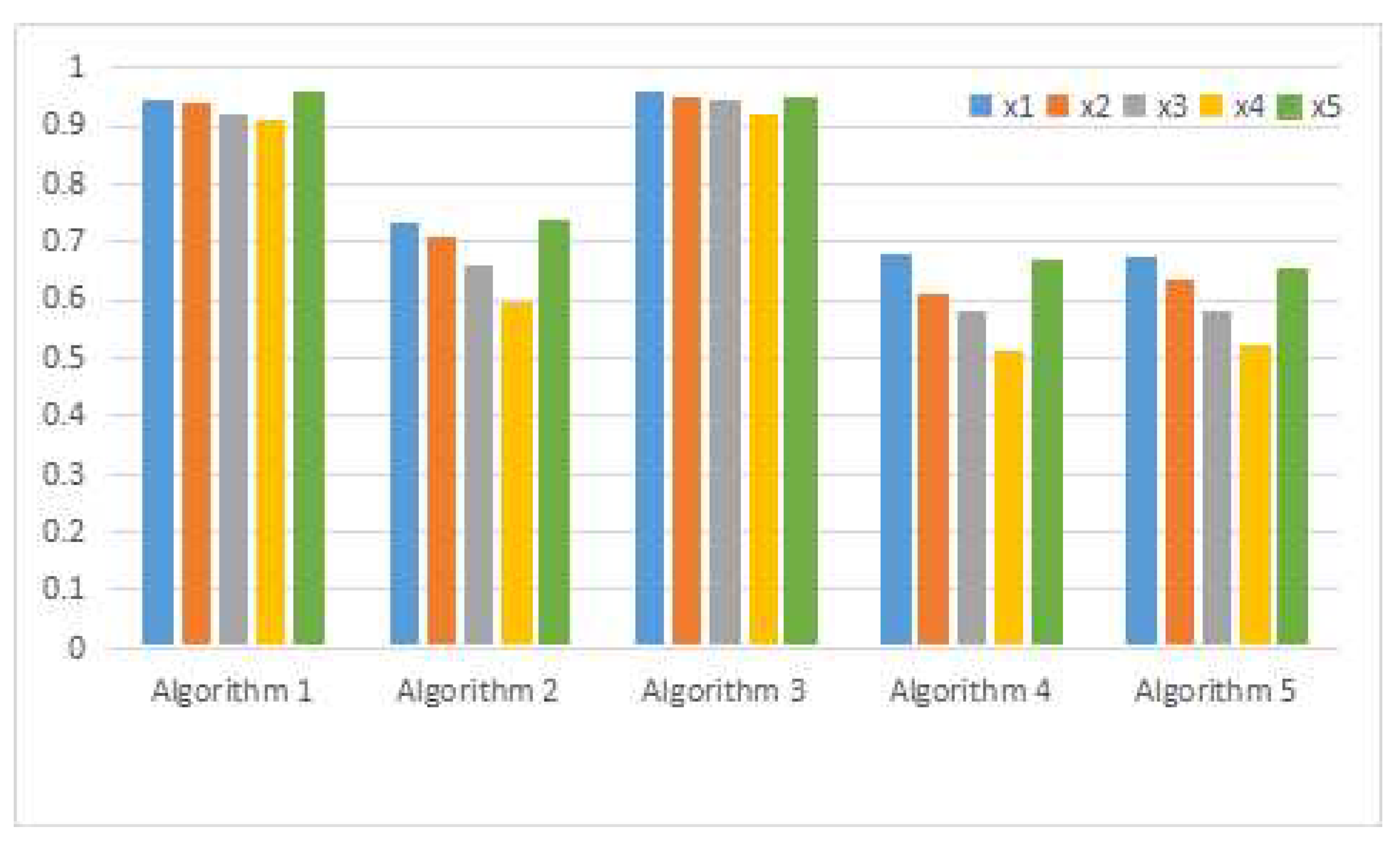
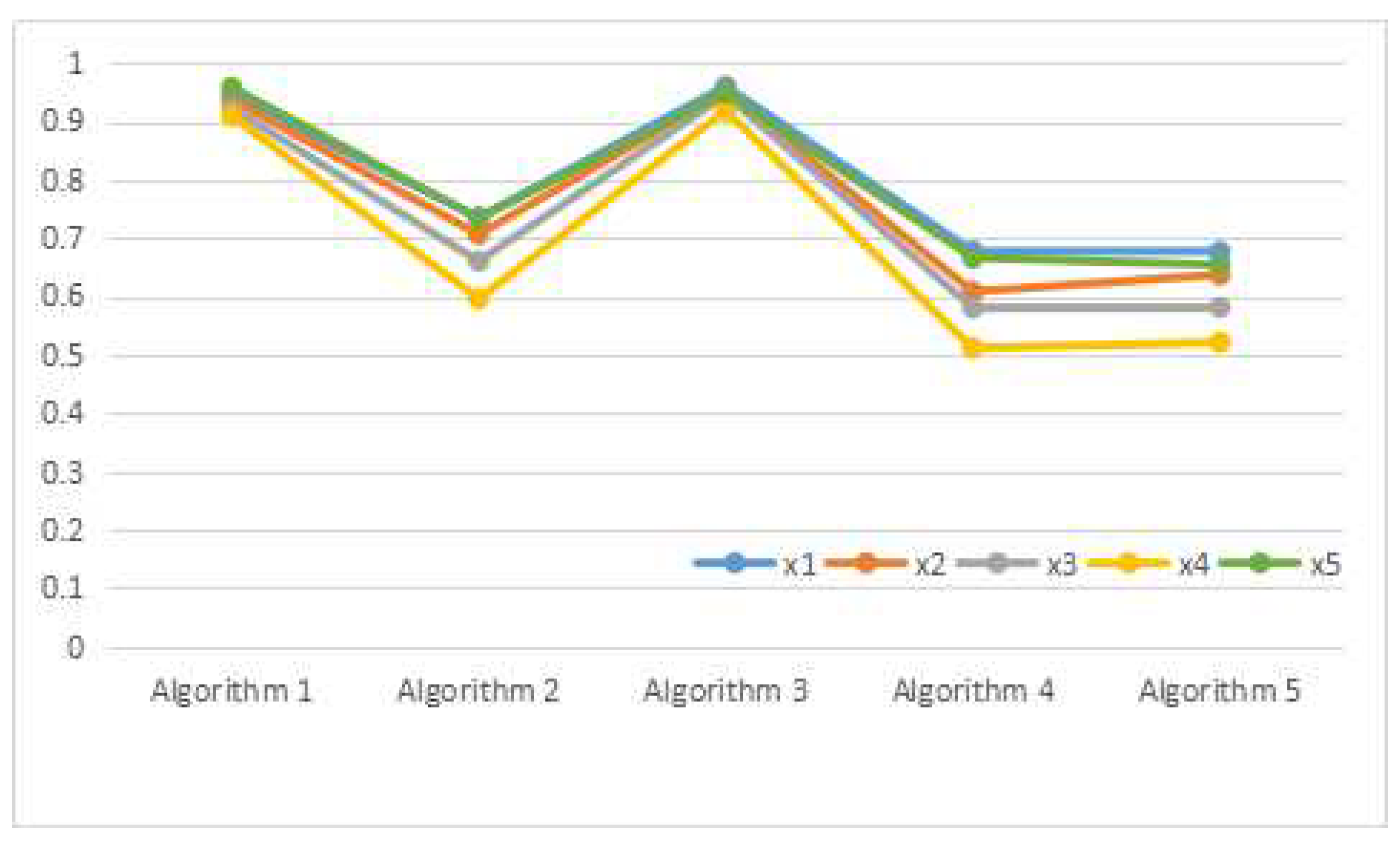
6.4. A Comparison Analysis

To validate the feasibility of the proposed decision making method, a comparative study was conducted with other methods. These methods, which were introduced by Liu [43], Yang et al. [32] and Ye [44], are compared with the proposed approach using SVN information system.

6.4.1. The Results of Liu’s Method

Liu’s method is shown in Algorithm 2.

Algorithm 2 The decision making algorithm [43].

Input: A SVN decision matrix D, a weight vector $\mathbf{w}$ and γ. Output: The score ordering for all alternatives.     1: Compute $$\begin{array}{ll}{n}_k& =\langle T_{n_k},I_{n_k},F_{n_k}\rangle [2mm]\hfill \\ & =HSVNNWA(n_{k1},n_{k2},\cdots ,n_{km})[2mm]\\ & =\langle \frac{\prod _{i=1}^m{(1+(\gamma -1)T_{ki})}^{w_i}-\prod _{i=1}^m{(1-T_{ki})}^{w_i}}{\prod _{i=1}^m{(1+(\gamma -1)T_{ki})}^{w_i}+(\gamma -1)\prod _{i=1}^m{(1-T_{ki})}^{w_i}},[2mm]\\ & \frac{\gamma \prod _{i=1}^m{I}_{ki}^{w_i}}{\prod _{i=1}^m{(1+(\gamma -1)(1-I_{ki}))}^{w_i}+(\gamma -1)\prod _{i=1}^m{I}_{ki}^{w_i}},[2mm]\\ & \frac{\gamma \prod _{i=1}^m{F}_{ki}^{w_i}}{\prod _{i=1}^m{(1+(\gamma -1)(1-F_{ki}))}^{w_i}+(\gamma -1)\prod _{i=1}^m{F}_{ki}^{w_i}}\rangle (k=1,2,\cdots ,l);\end{array}$$   2: Calculate $s(n_k)=\frac{T_{n_k}}{\sqrt{T_{n_k}^2+I_{n_k}^2+F_{n_k}^2}}$;   3: Obtain the ranking for all $s(n_k)$ by using the principle of numerical size and select the most possible patient.

Then, Algorithm 2 can be used for Example 10. Let $n_{ki}=\langle T_{ki},I_{ki},F_{ki}\rangle$ be the evaluation information of $x_k$ on $C_{{}_i}$ in Table 1. That is to say, Table 1 is the SVN decision matrix D. We suppose the weight vector of the criteria is $\mathbf{w}=(0.35,0,25,0.3,0.1)$ and $\gamma =1$.

Step 1: Based on HSVNNWA operator, we get

$$\begin{array}{c}{n}_1=\langle 0.557,0.178,0.482\rangle ,n_2=\langle 0.484,0.283,0.395\rangle ,\hfill \\ n_3=\langle 0.414,0.318,0.347\rangle ,n_4=\langle 0.465,0.286,0.558\rangle ,\hfill \\ n_5=\langle 0.578,0.233,0.486\rangle .\hfill \end{array}$$

Step 2: We get

$$s(n_1)=0.735,s(n_2)=0.706,s(n_3)=0.660,s(n_4)=0.596,s(n_5)=0.734$$

.

Step 3: According to the cosine similarity degrees $s(n_k)$ ($k=1,2,\cdots ,5$), we obtain $x_4<x_3<x_2<x_5<x_1$.

Therefore, Patient $x_1$ is more likely to be sick with Disease B.

6.4.2. The Results of Yang’s Method

Yang’s method is shown in Algorithm 3.

Algorithm 3 The decision making algorithm [32].

Input: A generalized SVN approximation space ($U,V,\tilde{R}$), $B\in SVN(V)$. Output: The score ordering for all alternatives.     1: Calculate the lower and upper approximations $\overline{\tilde{R}}(B)$ and $\underline{\tilde{R}}(B)$;   2: Compute $n_{x_k}=(\overline{\tilde{R}}(B)⨁\underline{\tilde{R}}(B))(x_k)$ ($k=1,2,\cdots ,l$);   3: Compute $$\begin{array}{c}s(n_{x_k},n^{*})=\frac{T_{n_{x_k}}·T_{n^{*}}+I_{n_{x_k}}·I_{n^{*}}+F_{n_{x_k}}·F_{n^{*}}}{\sqrt{T_{n_{x_k}}^2+I_{n_{x_k}}^2+F_{n_{x_k}}^2}·\sqrt{{(T_{n^{*}})}^2+{(I_{n^{*}})}^2+{(F_{n^{*}})}^2}}(k=1,2,\cdots ,l),\hfill \end{array}$$ where $n^{*}=\langle T_{n^{*}},I_{n^{*}},F_{n^{*}}\rangle =\langle 1,0,0\rangle$;   4: Obtain the ranking for all $s(n_{x_k},n^{*})$ by using the principle of numerical size and select the most possible patient.

For Example 10, we suppose Disease $B\in SVN(V)$ and $B=\frac{(0.3,0.6,0.5)}{y_1}+\frac{(0.7,0.2,0.1)}{y_2}+\frac{(0.6,0.4,0.3)}{y_3}+\frac{(0.8,0.4,0.5)}{y_4}$. According to Table 1, the generalized SVN approximation space ($U,V,\tilde{R}$) can be obtained in

Table 4. The generalized SVN approximation space ($U,V,\tilde{R}$).

$\tilde{\mathit{R}}$	${\mathit{x}}_1$	${\mathit{x}}_2$	${\mathit{x}}_3$	${\mathit{x}}_4$	${\mathit{x}}_5$
$y_1$	$\langle 0.7,0.2,0.5\rangle$	$\langle 0.5,0.3,0.2\rangle$	$\langle 0.4,0.5,0.2\rangle$	$\langle 0.6,0.1,0.7\rangle$	$\langle 0.3,0.2,0.6\rangle$
$y_2$	$\langle 0.6,0.2,0.4\rangle$	$\langle 0.5,0.2,0.8\rangle$	$\langle 0.2,0.3,0.6\rangle$	$\langle 0.4,0.5,0.7\rangle$	$\langle 0.7,0.3,0.5\rangle$
$y_3$	$\langle 0.4,0.1,0.5\rangle$	$\langle 0.4,0.5,0.4\rangle$	$\langle 0.5,0.2,0.4\rangle$	$\langle 0.3,0.6,0.5\rangle$	$\langle 0.6,0.3,0.5\rangle$
$y_4$	$\langle 0.1,0.5,0.6\rangle$	$\langle 0.6,0.1,0.7\rangle$	$\langle 0.6,0.3,0.4\rangle$	$\langle 0.5,0.3,0.2\rangle$	$\langle 0.8,0.1,0.2\rangle$

, where $U=\{x_1,x_2,x_3,x_4,x_5\}$ and $V=\{y_1,y_2,y_3,y_4\}$.

Step 1: We get

$$\begin{array}{c}\overline{\tilde{R}}(B)=\{\langle x_1,0.6,0.2,0.4\rangle ,\langle x_2,0.6,0.2,0.4\rangle ,\langle x_3,0.6,0.3,0.4\rangle ,\langle x_4,0.5,0.4,0.5\rangle ,\langle x_5,0.8,0.3,0.5\rangle \},\hfill \\ \underline{\tilde{R}}(B)=\{\langle x_1,0.5,0.6,0.5\rangle ,\langle x_2,0.3,0.6,0.5\rangle ,\langle x_3,0.3,0.5,0.5\rangle ,\langle x_4,0.6,0.6,0.5\rangle ,\langle x_5,0.6,0.6,0.5\rangle \}.\hfill \end{array}$$

Step 2:

$$\begin{array}{cc}\overline{\tilde{R}}(B)⨁\underline{\tilde{R}}(B)=\hfill & \{\langle x_1,0.80,0.12,0.20\rangle ,\langle x_2,0.72,0.12,0.20\rangle ,\langle x_3,0.72,0.15,0.20\rangle ,\langle x_4,0.80,0.24,0.25\rangle ,\hfill \\ & \langle x_5,0.92,0.18,0.25\rangle \}.\hfill \end{array}$$

Step 3: Let $n^{*}=\langle 1,0,0\rangle$. Then,

$$s(n_{x_1},n^{*})=0.960,s(n_{x_2},n^{*})=0.951,s(n_{x_3},n^{*})=0.945,s(n_{x_4},n^{*})=0.918,s(n_{x_5},n^{*})=0.948$$

.

Step 4:

$$s(n_{x_4},n^{*})<s(n_{x_3},n^{*})<s(n_{x_5},n^{*})<s(n_{x_2},n^{*})<s(n_{x_1},n^{*})$$

.

Therefore, Patient $x_1$ is more likely to be sick with Disease B.

6.4.3. The Results of Ye’s Methods

Ye presented two methods [44]. Thus, Algorithms 4 and 5 are presented for Example 10.

Algorithm 4 The decision making algorithm [44].

Input: A SVN decision matrix D and a weight vector $\mathbf{w}$. Output: The score ordering for all alternatives.     1: Compute $$\begin{array}{c}{W}_k(x_k,A^{*})=\frac{{\sum }_{i=1}^m{w}_i[a_{ki}·a_i^{*}+b_{ki}·b_i^{*}+c_{ki}·c_i^{*}]}{\sqrt{{\sum }_{i=1}^m{w}_i[a_{ki}^2+b_{ki}^2+c_{ki}^2]}·\sqrt{{\sum }_{i=1}^m{w}_i[{(a_i^{*})}^2+{(b_i^{*})}^2+{(c_i^{*})}^2]}}(k=1,2,\cdots ,l),\hfill \end{array}$$ where ${\alpha }_i^{*}=\langle a_i^{*},b_i^{*},c_i^{*}\rangle =\langle 1,0,0\rangle$ ($i=1,2,\cdots ,m$);   2: Obtain the ranking for all $W_k(x_k,A^{*})$ by using the principle of numerical size and select the most possible patient.

For Example 10, Table 1 is the SVN decision matrix D. We suppose the weight vector of the criteria is $\mathbf{w}=(0.35,0,25,0.3,0.1)$.

Step 1:

$$W_1(x_1,A^{*})=0.677,W_2(x_2,A^{*})=0.608,W_3(x_3,A^{*})=0.580,W_4(x_4,A^{*})=0.511,W_5(x_5,A^{*})=0.666.$$

Step 2: The ranking order of $\{x_1,x_2,\cdots ,x_5\}$ is $x_4<x_3<x_2<x_5<x_1$. Therefore, Patient $x_1$ is more likely to be sick with Disease B.

Algorithm 5 The other decision making algorithm [44].

Input: A SVN decision matrix D and a weight vector $\mathbf{w}$. Output: The score ordering for all alternatives.     1: Compute $$\begin{array}{c}{M}_k(x_k,A^{*})=\sum _{i=1}^m{w}_i\frac{a_{ki}·a_i^{*}+b_{ki}·b_i^{*}+c_{ki}·c_i^{*}}{\sqrt{a_{ki}^2+b_{ki}^2+c_{ki}^2}·\sqrt{{(a_i^{*})}^2+{(b_i^{*})}^2+{(c_i^{*})}^2}}(k=1,2,\cdots ,l),\hfill \end{array}$$ where ${\alpha }_i^{*}=\langle a_i^{*},b_i^{*},c_i^{*}\rangle =\langle 1,0,0\rangle$ ($i=1,2,\cdots ,m$);   2: Obtain the ranking for all $M_k(x_k,A^{*})$ by using the principle of numerical size and select the most possible patient.

By Algorithms 5, we have:

Step 1:

$$\begin{gathered} M_1(x_1,A^{*})=0.676,M_2(x_2,A^{*})=0.637,M_3(x_3,A^{*})=0.581, \\ {M}_4(x_4,A^{*})=0.521,M_5(x_5,A^{*})=0.654. \end{gathered}$$

Step 2: The ranking order of $\{x_1,x_2,\cdots ,x_5\}$ is $x_4<x_3<x_2<x_5<x_1$. Therefore, Patient $x_1$ is more likely to be sick with Disease B.

All results are shown in

Table 5. The results utilizing the different methods of Example 10.

Methods	The Final Ranking	The Patient Is Most Sick With the Disease B
Algorithm 2 in Liu [43]	$x_4,x_3,x_2,x_5,x_1$	$x_1$
Algorithm 3 in Yang et al. [32]	$x_4,x_3,x_5,x_2,x_1$	$x_1$
Algorithm 4 in Ye [44]	$x_4,x_3,x_2,x_5,x_1$	$x_1$
Algorithm 5 in Ye [44]	$x_4,x_3,x_2,x_5,x_1$	$x_1$
Algorithm 1 in this paper	$x_4,x_3,x_2,x_1,x_5$	$x_5$

, Figure 1 and Figure 2.

Liu [43] and Ye [44] presented the methods by SVN theory. In their methods, the ranking order would be changed by different $\mathbf{w}$ and γ. We as well as Yang et al. [32] used different rough set models to make the decision. Yang et al. present a SVN rough set model based on SVN relations, while we present a new SVN rough set model based on coverings. The results are different by Yang’s and our methods, although the methods are both based on an operator presented by Ye [44].

In any method, if there are more than one most possible patient, then each patient will be the optimal decision. In this case, we need other methods to make a further decision. By means of different methods, the obtained results may be different. To achieve the most accurate results, further diagnosis is necessary in combination with other hybrid methods.

7. Conclusions

This paper is a bridge, linking SVNSs and covering-based rough sets. By introducing some definitions and properties in SVN β-covering approximation spaces, we present two types of SVN covering rough set models. Then, their characterizations and matrix representations are investigated. Moreover, an application to the problem of DM is proposed. The main conclusions in this paper and the further work to do are listed as follows.

• Two types of SVN covering rough set models are first presented, which combine SVNSs with covering-based rough sets. Some definitions and properties in covering-based rough set model, such as coverings and neighborhoods, are generalized to SVN covering rough set models. Neutrosophic sets and related algebraic structures [47,48,49] will be connected with the research content of this paper in further research.
• It would be tedious and complicated to use set representations to calculate SVN covering approximation operators. Therefore, the matrix representations of these SVN covering approximation operators make it possible to calculate them through the new matrices and matrix operations. By these matrix representations, calculations will become algorithmic and can be easily implemented by computers.
• We propose a method to DM problems under one of the SVN covering rough set models. It is a novel method based on approximation operators specific to SVN covering rough sets firstly. The comparison analysis is very interesting to show the difference between the proposed method and other methods.

References

1. Pawlak, Z. Rough sets. Int. J. Comput. Inf. Sci. 1982, 11, 341–356. [Google Scholar]
2. Pawlak, Z. Rough Sets: Theoretical Aspects of Reasoning about Data; Kluwer Academic Publishers: Boston, MA, USA, 1991. [Google Scholar]
3. Bartol, W.; Miro, J.; Pioro, K.; Rossello, F. On the coverings by tolerance classes. Inf. Sci. 2004, 166, 193–211. [Google Scholar]
4. Bianucci, D.; Cattaneo, G.; Ciucci, D. Entropies and co-entropies of coverings with application to incomplete information systems. Fundam. Inform. 2007, 75, 77–105. [Google Scholar]
5. Zhu, W. Relationship among basic concepts in covering-based rough sets. Inf. Sci. 2009, 179, 2478–2486. [Google Scholar]
6. Yao, Y.; Zhao, Y. Attribute reduction in decision-theoretic rough set models. Inf. Sci. 2008, 178, 3356–3373. [Google Scholar] [Green Version]
7. Wang, J.; Zhang, X. Matrix approaches for some issues about minimal and maximal descriptions in covering-based rough sets. Int. J. Approx. Reason. 2019, 104, 126–143. [Google Scholar]
8. Li, F.; Yin, Y. Approaches to knowledge reduction of covering decision systems based on information theory. Inf. Sci. 2009, 179, 1694–1704. [Google Scholar]
9. Wu, W. Attribute reduction based on evidence theory in incomplete decision systems. Inf. Sci. 2008, 178, 1355–1371. [Google Scholar]
10. Wang, J.; Zhu, W. Applications of bipartite graphs and their adjacency matrices to covering-based rough sets. Fundam. Inform. 2017, 156, 237–254. [Google Scholar]
11. Dai, J.; Wang, W.; Xu, Q.; Tian, H. Uncertainty measurement for interval-valued decision systems based on extended conditional entropy. Knowl.-Based Syst. 2012, 27, 443–450. [Google Scholar]
12. Wang, C.; Chen, D.; Wu, C.; Hu, Q. Data compression with homomorphism in covering information systems. Int. J. Approx. Reason. 2011, 52, 519–525. [Google Scholar]
13. Li, X.; Yi, H.; Liu, S. Rough sets and matroids from a lattice-theoretic viewpoint. Inf. Sci. 2016, 342, 37–52. [Google Scholar]
14. Wang, J.; Zhang, X. Four operators of rough sets generalized to matroids and a matroidal method for attribute reduction. Symmetry 2018, 10, 418. [Google Scholar]
15. Wang, J.; Zhu, W. Applications of matrices to a matroidal structure of rough sets. J. Appl. Math. 2013, 2013, 493201. [Google Scholar]
16. Wang, J.; Zhu, W.; Wang, F.; Liu, G. Conditions for coverings to induce matroids. Int. J. Mach. Learn. Cybern. 2014, 5, 947–954. [Google Scholar]
17. Chen, J.; Li, J.; Lin, Y.; Lin, G.; Ma, Z. Relations of reduction between covering generalized rough sets and concept lattices. Inf. Sci. 2015, 304, 16–27. [Google Scholar]
18. Zhang, X.; Dai, J.; Yu, Y. On the union and intersection operations of rough sets based on various approximation spaces. Inf. Sci. 2015, 292, 214–229. [Google Scholar]
19. D’eer, L.; Cornelis, C.; Godo, L. Fuzzy neighborhood operators based on fuzzy coverings. Fuzzy Sets Syst. 2017, 312, 17–35. [Google Scholar] [Green Version]
20. Yang, B.; Hu, B. On some types of fuzzy covering-based rough sets. Fuzzy Sets Syst. 2017, 312, 36–65. [Google Scholar]
21. Zhang, X.; Miao, D.; Liu, C.; Le, M. Constructive methods of rough approximation operators and multigranulation rough sets. Knowl.-Based Syst. 2016, 91, 114–125. [Google Scholar]
22. Wang, J.; Zhang, X. Two types of intuitionistic fuzzy covering rough sets and an application to multiple criteria group decision making. Symmetry 2018, 10, 462. [Google Scholar]
23. Zadeh, L.A. Fuzzy sets. Inf. Control 1965, 8, 338–353. [Google Scholar]
24. Medina, J.; Ojeda-Aciego, M. Multi-adjoint t-concept lattices. Inf. Sci. 2010, 180, 712–725. [Google Scholar]
25. Pozna, C.; Minculete, N.; Precup, R.E.; Kóczy, L.T.; Ballagi, Á. Signatures: Definitions, operators and applications to fuzzy modeling. Fuzzy Sets Syst. 2012, 201, 86–104. [Google Scholar]
26. Jankowski, J.; Kazienko, P.; Watróbski, J.; Lewandowska, A.; Ziemba, P.; Zioło, M. Fuzzy multi-objective modeling of effectiveness and user experience in online advertising. Expert Syst. Appl. 2016, 65, 315–331. [Google Scholar]
27. Vrkalovic, S.; Lunca, E.C.; Borlea, I.D. Model-free sliding mode and fuzzy controllers for reverse osmosis desalination plants. Int. J. Artif. Intell. 2018, 16, 208–222. [Google Scholar]
28. Ma, L. Two fuzzy covering rough set models and their generalizations over fuzzy lattices. Fuzzy Sets Syst. 2016, 294, 1–17. [Google Scholar]
29. Wang, H.; Smarandache, F.; Zhang, Y.; Sunderraman, R. Single valued neutrosophic sets. Multispace Multistruct. 2010, 4, 410–413. [Google Scholar]
30. Atanassov, K. Intuitionistic fuzzy sets. Fuzzy Sets Syst. 1986, 20, 87–96. [Google Scholar]
31. Mondal, K.; Pramanik, S. Rough neutrosophic multi-attribute decision-making based on grey relational analysis. Neutrosophic Sets Syst. 2015, 7, 8–17. [Google Scholar]
32. Yang, H.; Zhang, C.; Guo, Z.; Liu, Y.; Liao, X. A hybrid model of single valued neutrosophic sets and rough sets: Single valued neutrosophic rough set model. Soft Comput. 2017, 21, 6253–6267. [Google Scholar]
33. Zhang, X.; Xu, Z. The extended TOPSIS method for multi-criteria decision making based on hesitant heterogeneous information. In Proceedings of the 2014 2nd International Conference on Software Engineering, Knowledge Engineering and Information Engineering (SEKEIE 2014), Singapore, 5–6 August 2014. [Google Scholar]
34. Cheng, J.; Zhang, Y.; Feng, Y.; Liu, Z.; Tan, J. Structural optimization of a high-speed press considering multi-source uncertainties based on a new heterogeneous TOPSIS. Appl. Sci. 2018, 8, 126. [Google Scholar]
35. Liu, J.; Zhao, H.; Li, J.; Liu, S. Decision process in MCDM with large number of criteria and heterogeneous risk preferences. Oper. Res. Perspect. 2017, 4, 106–112. [Google Scholar]
36. Watróbski, J.; Jankowski, J.; Ziemba, P.; Karczmarczyk, A.; Zioło, M. Generalised framework for multi-criteria method selection. Omega 2018. [Google Scholar] [CrossRef]
37. Faizi, S.; Sałabun, W.; Rashid, T.; Wa̧tróbski, J.; Zafar, S. Group decision-making for hesitant fuzzy sets based on characteristic objects method. Symmetry 2017, 9, 136. [Google Scholar]
38. Faizi, S.; Rashid, T.; Sałabun, W.; Zafar, S.; Wa̧tróbski, J. Decision making with uncertainty using hesitant fuzzy sets. Int. J. Fuzzy Syst. 2018, 20, 93–103. [Google Scholar]
39. Zhan, J.; Ali, M.I.; Mehmood, N. On a novel uncertain soft set model: Z-soft fuzzy rough set model and corresponding decision making methods. Appl. Soft Comput. 2017, 56, 446–457. [Google Scholar]
40. Zhan, J.; Alcantud, J.C.R. A novel type of soft rough covering and its application to multicriteria group decision making. Artif. Intell. Rev. 2018, 4, 1–30. [Google Scholar]
41. Zhang, Z. An approach to decision making based on intuitionistic fuzzy rough sets over two universes. J. Oper. Res. Soc. 2013, 64, 1079–1089. [Google Scholar]
42. Akram, M.; Ali, G.; Alshehri, N.O. A new multi-attribute decision-making method based on m-polar fuzzy soft rough sets. Symmetry 2017, 9, 271. [Google Scholar]
43. Liu, P. The aggregation operators based on archimedean t-conorm and t-norm for single-valued neutrosophic numbers and their application to decision making. Int. J. Fuzzy Syst. 2016, 18, 849–863. [Google Scholar]
44. Ye, J. Multicriteria decision-making method using the correlation coefficient under single-valued neutrosophic environment. Int. J. Gen. Syst. 2013, 42, 386–394. [Google Scholar]
45. Bonikowski, Z.; Bryniarski, E.; Wybraniec-Skardowska, U. Extensions and intentions in the rough set theory. Inf. Sci. 1998, 107, 149–167. [Google Scholar]
46. Pomykala, J.A. Approximation operations in approximation space. Bull. Pol. Acad. Sci. 1987, 35, 653–662. [Google Scholar]
47. Zhang, X.; Bo, C.; Smarandache, F.; Dai, J. New inclusion relation of neutrosophic sets with applications and related lattice structure. Int. J. Mach. Learn. Cybern. 2018, 9, 1753–1763. [Google Scholar]
48. Zhang, X. Fuzzy anti-grouped filters and fuzzy normal filters in pseudo-BCI algebras. J. Intell. Fuzzy Syst. 2017, 33, 1767–1774. [Google Scholar]
49. Zhang, X.; Park, C.; Wu, S. Soft set theoretical approach to pseudo-BCI algebras. J. Intell. Fuzzy Syst. 2018, 34, 559–568. [Google Scholar]
Figure 1. The first chat of different values of patient in utilizing different methods in Example 10.
Symmetry 10 00710 g001
Figure 2. The second chat of different values of patient in utilizing different methods in Example 10.
Symmetry 10 00710 g002