Article

Research on an Adaptive Variational Mode Decomposition with Double Thresholds for Feature Extraction

1
Software Institute, Dalian Jiaotong University, Dalian 116028, China
2
Co-Innovation Center of Shandong Colleges and Universities: Future Intelligent Computing, Yantai 264005, China
3
Traction Power State Key Laboratory of Southwest Jiaotong University, Chengdu 610031, China
4
Guangxi Key Lab of Multi-Source Information Mining & Security, Guangxi Normal University, Guilin 541004, China
5
Guangxi Key Laboratory of Hybrid Computation and IC Design Analysis, Guangxi University for Nationalities, Nanning 530006, China
6
Liaoning Key Laboratory of Welding and Reliability of Rail Transportation Equipment, Dalian Jiaotong University, Dalian 116028, China
*
Author to whom correspondence should be addressed.
Symmetry 2018, 10(12), 684; https://doi.org/10.3390/sym10120684
Submission received: 25 October 2018 / Revised: 13 November 2018 / Accepted: 14 November 2018 / Published: 1 December 2018
(This article belongs to the Special Issue Symmetry in Mechanical Engineering)

Abstract

:
A motor bearing system is a nonlinear dynamics system with nonlinear support stiffness. It is an asymmetry system, which plays an extremely important role in rotating machinery. In this paper, a center frequency method of double thresholds is proposed to improve the variational mode decomposition (VMD) method, then an adaptive VMD (called DTCFVMD) method is obtained to extract the fault feature. In the DTCFVMD method, a center frequency method of double thresholds is a symmetry method, which is used to determine the decomposed mode number of VMD according to the power spectrum of the signal. The proposed DTCFVMD method is used to decompose the nonlinear and non-stationary vibration signals of motor bearing in order to obtain a series of intrinsic mode functions (IMFs) under different scales. Then, the Hilbert transform is used to analyze the envelope of each mode component and calculate the power spectrum of each mode component. Finally, the power spectrum is used to extract the fault feature frequency for determining the fault type of the motor bearing. To test and verify the effectiveness of the DTCFVMD method, the actual fault vibration signal of the motor bearing is selected in here. The experimental results show that the center frequency method of double thresholds can effectively determine the mode number of the VMD method, and the proposed DTCFVMD method can accurately extract the clear time frequency characteristics of each mode component, and obtain the fault characteristics of characteristics; frequency, rotating frequency, and frequency doubling and so on.

1. Introduction

Time-frequency analysis method has been the most commonly applied method in the field of fault diagnosis of rotating machinery [1,2,3]. Vibration signals of rotating machinery usually contain a lot of information about the equipment health states. During equipment operation, when the equipment health state takes a turn for the worse, the impact and impact pulses of the equipment will increase [4,5,6]. Therefore, it is very significant to deeply analyze vibration signals for health monitoring and fault prediction of rotating machinery.
Due to the complex structure and changeable working conditions of rotating machinery, the vibration signals often take on the characteristics of multi-component and non-stationary. The time-frequency analysis method is widely applied to process the vibration signals of rotating machinery in order to extract fault features by using signal decomposition and filtering [7,8,9,10,11,12,13,14,15,16]. There exists a lot of time-frequency analysis methods, such as the Gabor transform, wavelet transform, Hilbert-Huang transform, empirical mode decomposition (EMD), local mean decomposition (LMD), empirical wavelet transform (EWT), and so on [17,18,19,20,21,22,23,24,25,26,27,28,29,30,31,32]. These time-frequency analysis methods can extract fault features from vibration signals, but they have their own problems in vibration signal analysis. The wavelet transform needs to select the wavelet basis function in advance, thus it is a non-adaptive signal analysis method. The applications of EMD and LMD are restricted because of the existence of mode mixing. Although the EEMD and ensemble LMD methods alleviate the mode mixing problem to a certain extent, the computation complexity is sharply increased and the added white noises cannot be removed. variational mode decomposition (VMD) is an adaptive and non-recursive signal decomposition method developed by Dragomiretskiy and Zosso in 2014 [33]. The VMD method is used to the transform mode decomposition problem into a variational solution problem. Additionally, the alternating direction multiplier method is used to optimize the VMD. The signal is decomposed into a k discrete number of sub-signals; near the corresponding center frequency, each component is considered to be tight. The constrained variational optimization problem is used to evaluate the bandwidth of the component. In the optimization, it can obtain a set of mode ensemble with the limited band feature. It is essentially a set of adaptive Wiener filter bank and can separate the modes with different center frequencies. Therefore, the VMD method is widely used to extract the principal modes for fault diagnosis in bearings’ signals. Wang et al. [34] studied the equivalent filtering characteristics of VMD, and proposed a rub-impact fault detection method for realizing rotor-stator fault diagnosis. Yi et al. [35] proposed a novel method of fault feature extraction based on the combination of VMD and the particle swarm optimization (PSO) algorithm. Liu et al. [36] proposed a novel signal denoising method that combines variational mode decomposition and detrended fluctuation analysis. Zhang et al. [37] proposed a novel hybrid fault diagnosis approach by using variational mode decomposition and majoriation-minization based total variation denoising for the denoising and non-stationary feature extraction. Liu et al. [38] proposed an improved variational mode decomposition for time-frequency analysis of fault diagnosis of a turbine rotor. Henao et al. [39] reviewed diagnostic techniques for electrical machines. An et al. [40] proposed a gear fault diagnosis method based on variational mode decomposition and envelope analysis according to the modulation characteristics of the gear vibration signal arising from faults therein. Mahgoun et al. [41] proposed a gear fault detection method by using the VMD method at a variable rotating speed. Abdoos et al. [42] proposed a new hybrid algorithm based on VMD, S-transform, and support vector machines for power quality disturbances’ detection in electrical power systems. Li et al. [43] proposed an independence-oriented VMD method for identifying the fault feature of the wheel set bearing of a high-speed locomotive. From the application of the VMD method, it can see that the VMD method can better extract the multiple features from a vibration signal. However, the VMD method needs to give the mode number in advance. If the given mode number is unreasonable, the VMD method will cause the loss of important modes. Now, the VMD method is widely used to analyze the signal, and the central frequency observation method is used to determine the appropriate mode number. In this method, a number of values of the mode number is preset to repeatedly run VMD several times, and then the results of all trials are observed to determine the appropriate value of the mode number. This method requires manual judgments and experience to determine the appropriate value of the mode number, thus it will greatly limit the adaptability of VMD method. In order to overcome this drawback, some researchers have deeply studied and improved the VMD method. Immovilli and Cocconcelli [44] investigated shaft radial load effect on bearing fault signatures’ detection. Wang et al. [45] proposed a complex variational mode decomposition method for the analysis of complex-valued data. Zhang et al. [46] proposed an improved VMD method with adaptive parameter selection to analyze vibration signals. Mohanty et al. [47] proposed a novel fault identification method based on combining variational mode decomposition, the Hurst exponent, and correlation coefficient. Choi et al. [48] proposed an improvement of variational mode decomposition that can effectively handle problems caused by missing values. Wang et al. [49] proposed a quasi-bivariate VMD method for extracting features with various scales. In addition, the other feature extraction methods are proposed in recent years [50,51,52].
These improved VMD methods can better determine the mode number and extract the multiple features from a vibration signal. However, some limitations remain regarding the adaptability of the VMD method. Therefore, it is necessary to continue to deeply study the appropriate mode number in the VMD. In this paper, a method called VMD with the center frequency method of double thresholds (DTCFVMD) is proposed to determine the appropriate mode number. Then, the DTCFVMD method is introduced into signal analysis to identify the bearing fault type. Finally, the actual fault vibration signal of the motor bearing is selected to test and verify the effectiveness of the DTCFVMD method.

2. Basic Methods

2.1. Variational Mode Decomposition (VMD) Method

The VMD method is an adaptive signal decomposition method by Dragomiretskiy and Zosso [33]. It is used to decompose a real signal into a set of sub-signals. Near the corresponding center frequency, each component is considered to be tight. The constrained variational optimization problem is used to evaluate the bandwidth of the component. Finally, in the optimization, the VMD method can obtain a solution for the constrained variational problem.
In the VMD method, the intrinsic mode function (IMF) is defined as an amplitude modulation- amplitude frequency (AM-FM) signal. Its expression is described as follows:
u k ( t ) = A k ( t ) cos ( φ k ( t ) )  
where, φ k ( t ) is a non-decreasing function, φ k ( t ) 0 , A k ( t ) is the envelopment; the change of the envelopment, A k ( t ) , and the instantaneous frequency, w k ( t ) = φ k ( t ) , is much slower than the phase, φ k ( t ) . In other words, in sufficiently long intervals, [ t δ , t + δ ] , δ 2 π / φ k ( t ) , u k ( t ) can be regarded as a pure harmonic signal with the amplitude, A k ( t ) , and frequency, w k ( t ) .
To evaluate the bandwidth of the mode, for each mode function, u k ( t ) , the Hilbert transform is used to obtain the unilateral spectrum of the signal, ( δ ( t ) + j / π t ) u k ( t ) . δ ( t ) is the distribution function of Dirichlet, * represents the convolution. An exponential term, e j w k t , is added to adjust the estimated center frequency of each mode function of the corresponding analytic signal, and the spectrum of each mode is transferred to the base band, [ ( δ ( t ) + j / π t ) u k ( t ) ] e j w k t . w k represents the center frequency. Then, the Gauss smoothing of the signal is demodulated to obtain the constraint variational problem.
min { u k } , { w k } { k | | t [ ( δ ( t ) + j π t ) u k ( t ) ] e j w k t | | 2 2 }  
subject to:
k u k = f  
To transform the constraint problem into an unconstrained problem, Lagrangian multipliers, λ , and quadratic penalty term, α , are applied to render the unconstrained variational problem. The Lagrangian multipliers, λ , can strictly enforce constraints. The quadratic penalty, α , can ensure the reconstruction accuracy. The augmented Lagrangian is described as:
L ( { u k } , { w k } , λ ) = α k t [ ( δ ( t ) + j π t ) u k ( t ) ] e j w k t 2 2 + f ( t ) k u k ( t ) 2 2 + < λ ( t ) , f ( t ) k u k ( t ) >  
In VMD, the alternating direction method of the multiplicative operator is used to solve the above variational problem. The mode function, u k n + 1 , center frequency, w k n + 1 , and λ are alternated and updated to seek to expand the saddle point of the Lagrange expression. The value problem of the mode function, u k n + 1 , is described as:
u k n + 1 = arg min u k X { α k t [ ( δ ( t ) + j π t ) u k ( t ) ] e j w k t 2 2 + f ( t ) k u k ( t ) + λ ( t ) 2 2 2 }  
The equidistance transformation of Parseval/Plancherel Fourier is used to transform the formula (4) into the frequency domain.
u ^ k n + 1 = arg min u ^ k , u k X { α j ( w ) [ ( 1 + s n g ( w + w k ) ) u ^ k ( w + w k ) 2 2 + f ^ ( w ) i u ^ i ( w ) + λ ^ ( t ) 2 2 2  
The w in the first item is replaced by w w k to obtain the following expression:
u ^ k n + 1 = arg min u ^ k , u k X { α j ( w w k ) [ ( 1 + s n g ( w ) ) u ^ k ( w ) 2 2 + f ^ ( w ) i u ^ i ( w ) + λ ^ ( t ) 2 2 2  
In the approximation terms of reconstruction, the conjugate symmetry of real signals is used to transform the expression (7) into the form of a non-negative frequency integral.
u ^ k n + 1 = arg min u ^ k , u k X { 0 4 α ( w w k ) 2 | u ^ k ( w ) | 2 + 2 | f ^ ( w ) i u ^ i ( w ) + λ ^ ( w ) 2 | 2 d w }  
By conversion, the solution of quadratic optimization problem can be obtained as follows:
u ^ k n + 1 ( w ) = ( ( f ^ ( w ) i = k u ^ i ( w ) + λ ^ ( w ) 2 ) 1 1 + 2 α ( w w k ) 2  
where, u ^ k n + 1 ( w ) is equivalent to the wiener filtering of the current residualwiener filtering equivalent to the current residual, f ^ ( w ) i = k u ^ i ( w ) . The full spectrum of the real mode can be completed symmetrically by Hermite symmetry, and the u ^ k ( w ) is the real part, u k ( t ) , of the inverse Fourier transform.
The center frequency, w k , is the first item of the right side of the expression (5) and the expression (6). Therefore, the updated expression, w k , is described as follows:
w k n + 1 = arg min w k { k t [ ( δ ( t ) + j π t ) u k ( t ) ] e j w k t 2 2 }  
It is like as the mode function, u k , and the center frequency, w k , in the Fourier domain is optimized as follows:
w k n + 1 = arg min w k { 0 ( w w k ) 2 | u ^ k ( w ) | 2 d w }  
The solution of the above quadratic optimization problem is given:
w k n + 1 = 0 w | u ^ k ( w ) | 2 d w 0 | u ^ k ( w ) | 2 d w  
The algorithm process of VMD is described as the follows:
Step 1. Initialize the parameters of VMD, including { u ^ k 1 } , { w k 1 } , and n .
Step 2. Update the u k and w k according to the expression (9) and expression (12).
Step 3. Update the λ .
λ ^ n + 1 ( w ) λ ^ n ( w ) + τ ( f ^ ( w ) k u ^ k n + 1 ( w ) )  
Step 4. Set the error to ε > 0 . If k | | u ^ k n + 1 u ^ k n | | 2 2 | | u ^ k n | | 2 2 < ε is met, the iteration is terminated. Otherwise, return to Step 2.

2.2. Empirical Mode Decomposition and Ensemble Empirical Mode Decomposition

The EMD method is an adaptive decomposition method. The EMD method can decompose non-linear data into a series of amplitude modulated-frequency modulated (AM-FM) components. The EMD decomposes the original signal (S(x)) into a number of IMFs:
S ( t ) = i = 1 n c i ( t ) + r n ( t )  
where rn(t) represents residual error function, and IMF components, c 1 , c 2 , c 3 , , c n , contain different elements, respectively, from a low to high frequency of signals.
The EEMD method is an improved EMD method [53,54]. It can solve the mode mixing problem in the VMD method by adding Gaussian white noise. The decomposition principle of the EEMD method is that the additional white noise is uniformly distributed in the whole time-frequency space, and the time-frequency space is composed of different scale components separated by the filter group. When the signal is added with a uniformly distributed white noise, the signal regions under different scales are automatically mapped to the appropriate scales.

3. An Adaptive VMD with the Center Frequency Method of Double Thresholds

Compared with the EMD and EEMD methods, VMD is a new signal decomposition method. This method has a better theoretical basis. Its essence is multiple adaptive Wiener filter banks, which take on better noise robustness. In the field of mode decomposition, the VMD can successfully separate two pure harmonic signals with similar frequencies and effectively suppress the mode mixing. However, the VMD decomposition needs to set the number of the decomposition in advance. How to effectively determine the number of the decomposition will directly affect the final decomposition results. If the presupposed value of it is greater than the effective mode number in the signal, it will generate the excessive decomposition phenomenon, decomposing the useless false components to interfere with the analysis of the effective components in the original signal. If the presupposed value is less than the effective mode number in the signal, it will generate the undecomposed phenomenon, which cannot completely decompose the effective component. Therefore, it is a very important role to determine the mode number of the VMD method. The research of the VMD method has just started, and it is a research hotspot topic to determine the mode number for the VMD method at present. There are some methods, which are used to determine the mode number, such as the central frequency method, kurtosis method, and optimization algorithms, and so on. The central frequency value of the corresponding IMF component can be obtained by using the VMD decomposition. The central frequency method can directly determine the mode number by using the central frequency value obtained by VMD decomposition, so the central frequency method has been widely used. However, the central frequency method depends on the subjective factors when the mode number is selected. Therefore, on the basis of the central frequency method, the dual threshold of the central frequency method is proposed for the adaptive selection mode number in the VMD decomposition. The central frequency method of double thresholds is proposed to adaptively select the mode number in the VMD decomposition.

3.1. The Center Frequency Method

3.1.1. The Basic Principle and Implementation Steps

Each IMF component obtained by VMD decomposition corresponds to a central frequency, c f , and the center frequency of the decomposed IMF component under each scale is distributed from low frequency to high frequency. Set the maximum value, k max , of the decomposition scale, k , and the signal is decomposed under the decomposition scale, k = 1 , 2 , 3 , , k max . If the difference between the maximum value of the central frequency of the IMF component under the scale, k , and the maximum value of the central frequency of the IMF component under the scale, k + 1 , is very small, the IMF component under the scale, k , is determined to firstly obtain the maximum value of the central frequency. According to the central frequency method, the number, k , of the VMD decomposition is determined.
The implementation steps of the central frequency method are described as follows:
Step 1. Determine the maximum value, k max , of the decomposition scale.
Step 2. The VMD method is used to decompose the original signal into a series of IMF components under different scales ( I M F k ( k = 1 , 2 , 3 , , k max ) ). The central frequency values of each IMF component are calculated to obtain the set, Δ c f I M F k ( k = 1 , 2 , 3 , , k max ) .
Step 3. Calculate the maximum value of the center frequency of the set, c f I M F k , under different scales, as Δ c f _ max I M F k ( k = 1 , 2 , 3 , , k max ) .
Step 4. Calculate the maximum values of the center frequencies of the set, Δ c f _ max I M F k , as Δ c f _ max I M F .
Step 5. Calculate the difference between the maximum center frequency value of all modes and the maximum center frequency value of the mode under scale, k , as Δ c f _ max I M F K = Δ c f _ max I F M Δ c f _ max I F M k . If there is Δ c f _ max k < < Δ c f _ max I M F , the k is the mode decomposition number of the VMD method.
When the central frequency method is used to determine the mode number, k , it is necessary to determine the value, k , according to the Δ c f _ max k < < c f _ max I F M k . In the process, the subjective factors are influenced by human factors. The result will be that the optimal value cannot be obtained to some extent.

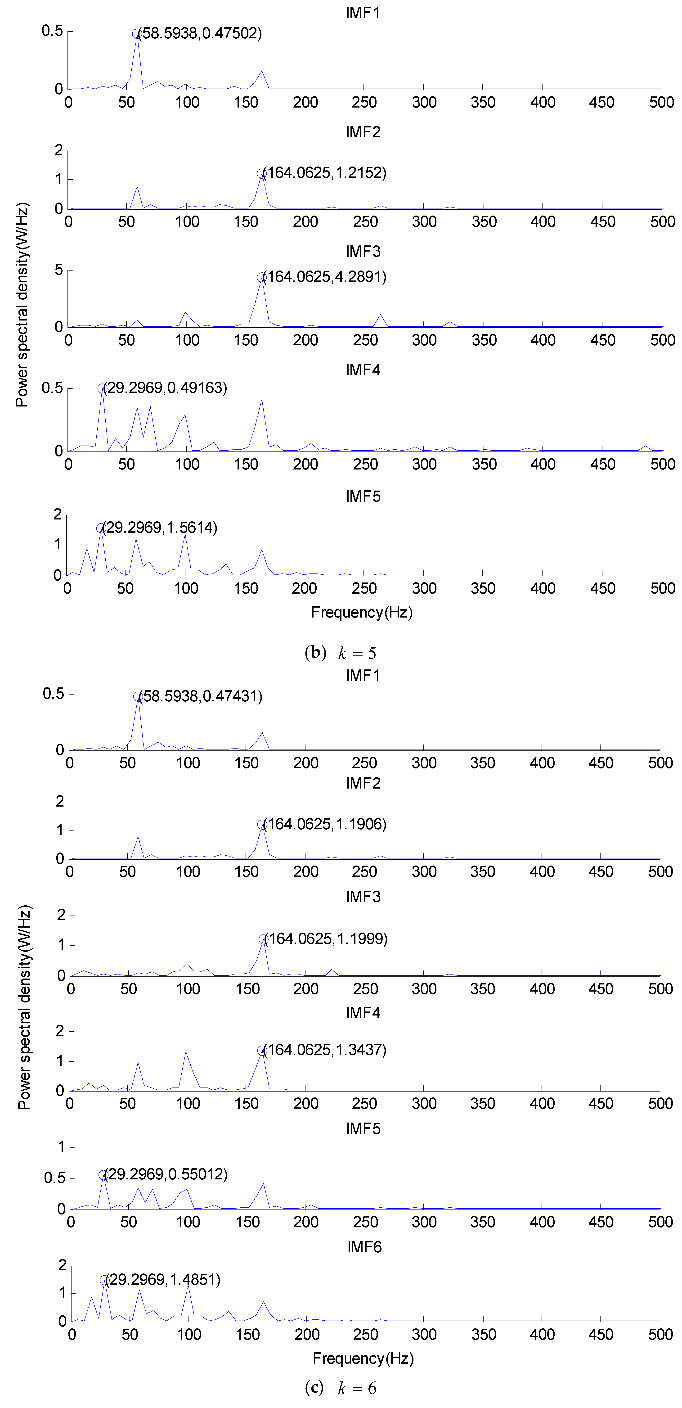
3.1.2. Experimental Analysis

The experiment data comes from the Bearing Data Center of Case Western Reserve University [55]. The deep groove ball bearing of 6205-2RS 6 JEM SKF (SKF company, Goteborg, Sweden) was used in this experiment. The experimental platform is shown in Figure 1. The motor with 1.5 Kw was connected to a dynamometer. The accelerometers at the 12 o’clock position on the drive end and fan end of motor housing were used to collect vibration data. The electro-discharge machining method was used to make the bearing’s inner race fault and outer race fault. The bearing information bearing is described in Table 1. The vibration signals were obtained under no-load (0 hp) at a rotating speed of 1797 r/min. The fault diameter was 0.1778 mm. The inner race fault and outer race fault vibration signals are selected in here. The vibration signals were sampled at 12,800 Hz. Each vibration signal duration was 10 s. The vibration signals were divided into sample segmentations. Each sample covered 2048 data points.
The theoretical calculation values of the fault characteristic frequency were calculated according to the calculation method, as shown in Table 2.
The inner race and outer race faults of the roller bearing are similar in Figure 2 and Figure 3.
The time domain waveform and frequency domain waveform of the inner race fault vibration signal are shown in Figure 4 and Figure 5.
Firstly, the VMD method was used to decompose the inner race fault vibration signal to obtain the central frequency of each IMF component under different scales, as shown in Figure 6.
As can be seen from Figure 6, when there is k = 7 , the center frequency of the seventh IMF component obtains the maximum value of all IMF components. When there is k 3 , the difference between the maximum value of the central frequency of the IMF component and the maximum value of all IMF components is very small under different scales. According to the center frequency method, the value of k is determined as k = 3 . When there is k 4 , the new frequency value appears in the mode. The analysis considers that the corresponding mode of the new frequency value is the effective mode. Therefore, when there is k = 3 , the effective mode cannot be completely decomposed. From the experimental results, it can be found that there is an undecomposed phenomenon for determining the value of k by using the central frequency method.
When the value of k is 5, the time domain waveform and frequency domain waveform of the inner race fault vibration signal are shown in Figure 7 and Figure 8.

3.2. The Center Frequency Method of Double Thresholds

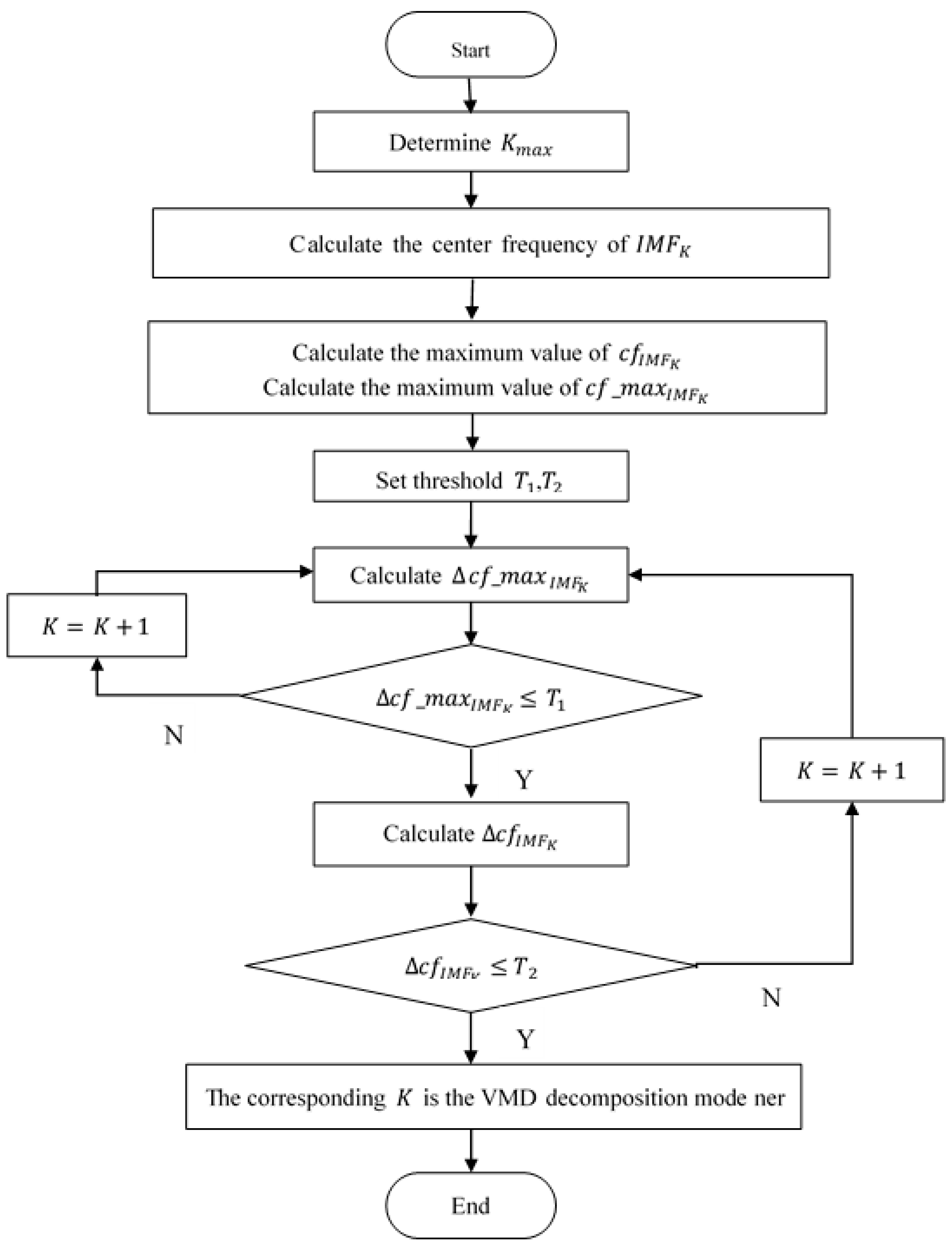
3.2.1. The Idea of the Center Frequency Method of Double Thresholds

For the shortcomings of the center frequency method, a center frequency method of double thresholds is proposed to determine the value of the decomposition scale, k , in this paper. The center frequency method of double thresholds is a symmetry method. Based on the center frequency, the double thresholds of T 1 and T 2 are set. The threshold, T 1 , is used to measure the difference between the maximum value of the central frequency of the corresponding modes under different scales and the maximum value of center frequencies of all modes. It is known by the central frequency method that the center frequency of the obtained IMF component under a certain scale is distributed from low frequency to high frequency. If the difference is greater than T 1 , it indicates that the maximum IMF component of the central frequency in the original signal is not decomposed. The threshold, T 2 , is used to measure the difference between the value of the central frequency of the L th IMF component and the value of the central frequency of the ( L 1 ) th IMF component under the same decomposition scale, k ( k = L ). The VMD can effectively decompose the two pure harmonic signals with similar frequencies, and the IMF components with similar frequencies are retained according to the threshold, T 2 . Set the maximum value, k max , of the decomposition scale, k . The signal is decomposed under decomposition scale, k = 1 , 2 , 3 , , k max , to obtain the value and the maximum value of the center frequency of the corresponding modes, and the maximum value of the center frequency of all modes under different scales. If the difference between the maximum value of the central frequency of the IMF component under a certain scale, k , and the maximum value of the central frequency of the IMF component under a certain scale, k + 1 , is less than T 1 , the difference between the value of the center frequency of the L th IMF component and the value of the center frequency of the ( L 1 ) th IMF component under the decomposition scale, k , is calculated ( k = L ). If the difference value is less than the threshold, T 2 , the minimum value of k meeting the above conditions is regarded as the optimal mode number of the VMD decomposition. The expressions of T 1 and T 2 are described as follows:
T 1 = a c f _ max I M F k      
T 2 = b c f _ max I M F k  
where there is k = 1 , 2 , 3 , , k max .
In a practical application, according to the different application backgrounds, the values of a and b are determined according to the experiences. Therefore, according to the practical application in this paper, there are a = 0.08 and b = 0.15 .

3.2.2. The Flow and Steps of the Center Frequency Method of Double Thresholds

The flow of the center frequency method of double thresholds is shown in Figure 9.
The implementation steps of the center frequency method of double thresholds are as follows:
Step 1. Determine the maximum value, k max , of the decomposition scale.
Step 2. The VMD method is used to decompose the original signal into a series of IMF components under different scales ( I M F k ( k = 1 , 2 , 3 , , k max ) ). The central frequency values of each IMF component is calculated to obtain the set, c f I M F k ( k = 1 , 2 , 3 , , k max ) .
Step 3. Calculate the maximum value of the center frequency of the set, c f I M F k , under different scales, as c f _ max I M F k ( k = 1 , 2 , 3 , , k max ) .
Step 4. Calculate the maximum value of the center frequency of the set, c f _ max I M F k , as c f _ max I M F .
Step 5. Set thresholds, a = 8 % and b = 15 % , for the expressions (15) and (16).
Step 6. Calculate the difference between the maximum center frequency value of all modes, as Δ c f _ max I M F k = c f _ max I F M c f _ max I F M k ( k = 1 , 2 , 3 , , k max ) .
Step 7. If there is Δ c f _ max k T 1 , Step 8 is executed. Otherwise, execute k = k + 1 and go to Step 6.
Step 8. Calculate the difference value of the central frequency of the L th IMF component and the value of the central frequency of the ( L 1 ) th IMF component of the set, c f I M F ( k = L ), and is calculated as Δ c f I M F = c f I M F k L c f I M F k L 1 . If there is Δ c f I M F T 2 , the corresponding k ( k = 1 , 2 , 3 , , k max ) of Δ c f I M F is the optimal mode number of the VMD method. Otherwise, execute k = k + 1 and go to Step 6.

3.3. Effectiveness Analysis of the Center Frequency Method of Double Thresholds

The center frequency method of double thresholds is used to determine the number of VMD decomposition modes. When there is k = 2 , the Δ c f _ max I M F k T 1 is not be met. When there is k = 3 , 4 , the Δ c f _ max I M F k T 2 is not be met. When there is k = 5 , the condition of judgment is met at the same time. Therefore, k = 5 is the optimal mode number of VMD decomposition. Compared with the central frequency method, the difference of the maximum value of the central frequency of the IMF component in the determined modes by two methods is very small, which shows that the component of the maximum value of the central frequency in the original signal has been decomposed. When there is k = 5 , the central frequency value of two additional IMF components did not appear in k = 3 . Therefore, the k = 5 is better than k = 3 according to the effective mode.
The time domain waveform and frequency domain waveform of the outer race fault vibration signal are shown in Figure 10 and Figure 11.
The outer race fault vibration signal is decomposed by VMD, and the central frequency value of each IMF component under different scales are shown in Figure 12.
As can be seen from Figure 12, when there is k = 7 , the center frequency value of the seventh IMF component obtains the maximum value of all IMF components. When there is k 2 , the difference between the maximum value of the central frequency of the IMF component and the maximum value of all IMF components is very small under different scales. According to the center frequency method, the value of k is determined as k = 2 . When there is k 3 , the new frequency value appears in the mode. The analysis considers that the corresponding mode of the new frequency value is the effective mode. Therefore, when there is k = 2 , the effective mode cannot be completely decomposed. The center frequency method of double thresholds is used to determine the number of VMD decomposition modes. When there is k = 2 , 3 , the Δ c f _ max I M F k T 2 is not be met. When there is k = 4 , the condition of judgment is met at the same time. Therefore, k = 4 is the optimal mode number of VMD decomposition. Compared with the central frequency method, the difference of the maximum value of the central frequency of the IMF component in the determined modes by the two methods is very small, which shows that the component of the maximum value of the central frequency in the original signal has been decomposed. When there is k = 4 , the central frequency value of two additional IMF components did not appear in k = 2 . Therefore, the k = 4 is better than k = 2 according to the effective mode.
When the value of k is 4, the time domain waveform and frequency domain waveform of the outer race fault vibration signal are shown in Figure 13 and Figure 14.
From the above experimental results and analysis, it can be found that the mode number of VMD with the central frequency method of double thresholds is superior to the mode number of VMD with the central frequency method. In the VMD method, the central frequency method of double thresholds can effectively solve the problem that the person determines the value of k according to Δ c f _ max k < < Δ c f _ max I M F k . At the same time, the central frequency method of double thresholds makes up for the defect that the central frequency method cannot keep the IMF components with similar frequency values. Therefore, the central frequency method of double thresholds can determine the value of k in the maximum extent, which is the optimal mode number.

4. Feature Extraction Method Based on the DTCFVMD and Hilbert Transform

4.1. Feature Extraction Method

When the rolling bearings have a fault, its vibration signal contains a lot of running state information, which are non-stationary and multicomponent modulation signals. Due to the weak modulation source, early fault signals and noise interference from surrounding equipment and the environment, it is difficult to extract and identify the fault feature frequency. The VMD method is an adaptive and non-recursive signal decomposition method. It adopts a completely non-recursive method to realize the frequency domain decomposition of a signal, which has a strong decomposition ability, good anti-noise performance, and fast processing speed. Therefore, the proposed DTCFVMD method is used to decompose the nonlinear and non-stationary vibration signals of bearings to obtain a series of intrinsic mode functions under different scales. Then, the Hilbert transform is used to analyze the envelope of each mode component and calculate the power spectrum of each mode component, which is used to extract the fault feature frequency for determining the fault type of the motor bearing. The feature extraction model based on the DTCFVMD and Hilbert transform is shown in Figure 15.

4.2. Steps of Feature Extraction

The steps of the feature extraction model based on the DTCFVMD and Hilbert transform are described as follows:
Step 1. Preprocess the collected vibration signals of the motor rolling bearing, including de-noising, filtering, and so on.
Step 2. Propose a center frequency method of double thresholds to improve the VMD method for obtaining the adaptive VMD(DTCFVMD) method.
Step 3. The preprocessed vibration signal is decomposed by using the proposed DTCFVMD method to obtain a series of IMFs.
Step 4. Analyze the envelope of each mode component by using the Hilbert transform.
Step 5. Calculate the power spectrum of each mode component to extract the fault feature frequency.
Step 6. The fault feature frequency is compared with theoretical inherent fault frequency to accurately determine the fault type of the motor rolling bearing.

5. Verification and Results Analysis

5.1. The Effectiveness Verification

The power spectrum represents the relationship between signal power and frequency; that is, the distribution of the signal power in the frequency domain. The Hilbert transform is used to solve the envelope of each IMF component, then the power spectrum of the envelope is solved. The maximum frequency value of the power spectral density is marked in order to express the fault characteristic frequency, rotating frequency, and frequency multiplication by power spectrum analysis.
According to the center frequency method of double thresholds, the optimal mode number of VMD decomposition for the inner race vibration signal and outer race vibration signal are 5 and 4, respectively. In order to verify the validity of the optimal mode, the signal power spectrum is used to extract the fault characteristic and estimate the effective frequency.
For the inner race fault vibration signal, the power spectrum of each IMF component under k = 4 , k = 5 , and k = 6 is shown in Figure 16 and Table 3.
As can be seen from Figure 16 and Table 3, 29.3 Hz represents the rotating frequency, 58.6 Hz represents the frequency doubling of the rotating frequency, and 164.1 Hz represents the fault characteristic frequency of the inner race. When there is k = 5 , the rotating frequency can be obtained from the frequency spectrum, but the rotating frequency cannot be obtained from the frequency spectrum when there is k = 4 . When there are k = 5 and k = 6 , the rotating frequency, the frequency doubling of the rotating frequency, and the fault characteristic frequency of the inner race can be obtained from the frequency spectrum. When there is k = 6 , it has one more fault characteristic frequency at 164.1 Hz than k = 5 . However, the frequency value repeats, so k = 5 is the optimal mode number of the VMD decomposition.
For the outer race vibration signal, the power spectrum of each IMF component under k = 4 , k = 5 , and k = 6 is shown in Figure 17 and Table 4.
As can be seen from Figure 17 and Table 4, 29.3 Hz represents the rotating frequency, 87.9 Hz represents the frequency tripling of the rotating frequency, 105.5 Hz represents the fault characteristic frequency of the outer race, and 46.9 Hz represents the difference between the fault characteristic frequency and the frequency doubling of the rotating frequency of the outer race. When there is k = 4 , the rotating frequency can be obtained from the frequency spectrum, but the rotating frequency cannot be obtained from the frequency spectrum when there is k = 3 . When there are k = 4 and k = 5 , the frequency tripling of the rotating frequency, the difference between the fault characteristic frequency, and the frequency doubling of the rotating frequency of the outer race can be obtained from the frequency spectrum. When there is k = 5 , it is not able to obtain the rotating frequency. Therefore, k = 4 is the optimal mode number of the VMD decomposition.
The frequency value of each IMF component extracted from the power spectrum shows that the value of k determined by the central frequency method of double thresholds is the optimal mode number of the VMD method. Therefore, it is proved that the proposed central frequency method of double thresholds is effective.

5.2. Comparison and Analysis

To verify the effectiveness of VMD with the center frequency method of double thresholds, the VMD with the center frequency method of double thresholds (DTCFVMD) is compared with the EMD and EEMD methods. The DTCFVMD, EMD, and EEMD methods are used to decompose the vibration signals of the inner ring and outer ring to obtain a series of IMFs. Then, the Hilbert transform is used to obtain the power spectrum of the decomposed IMF components. The effectiveness of DTCFVMD is explained by analyzing the effective frequency components extracted from the power spectrum.
The frequency values extracted by the power spectrum of each IMF component of the inner race vibration signal by using the DTCFVMD ( k = 5 ), EMD, and EEMD methods are shown in Table 5.
In Table 5, 29.3 Hz represents the rotating frequency, 58.6 Hz represents the frequency doubling of the rotating frequency, and 164.1 Hz represents the fault characteristic frequency of the inner race. As can be seen from Table 5, the number of effective frequencies of the power spectrum in the IMF component by using the EEMD method is more than that of the EMD method. Therefore, the decomposition effect of the EEMD method is better than that of the EMD method. Compared with the DTCFVMD method, the number of effective frequencies of IMF components by using the EEMD method is less than that of the EMD method and the EEMD method, and each mode can extract the effective frequency value. However, there exists some invalid frequency values in the modes of the EMD decomposition and the EEMD decomposition. In general, the decomposition effect of the DTCFVMD method is better than the decomposition effect of the EMD method and the EEMD method.
The frequency values extracted by the power spectrum of each IMF component of the outer race vibration signal by using the DTCFVMD ( k = 4 ), EMD, and EEMD methods are shown in Table 6.
In Table 6, 29.3 Hz represents the rotating frequency, 87.9 Hz represents the frequency tripling of the rotating frequency, 105.5 Hz represents the fault characteristic frequency of the outer race, 52.7 Hz represents the fault characteristic frequency of 1/2, 11.7 Hz represents the fault characteristic frequency of 1/9, and 46.9 Hz represents the difference between the fault characteristic frequency and the frequency doubling of the rotating frequency of the outer race. As can be seen from Table 6, the number of effective frequencies of the power spectrum in the IMF component by using the EEMD method is more than that of the EMD method, and the EEMD method can obtain the rotating frequency. Therefore, the decomposition effect of the EEMD method is better than that of the EMD method. Compared with the DTCFVMD method, the number of effective frequencies of IMF components by using the EEMD method is less than that of the EMD method and the EEMD method, and each mode can extract the effective frequency value. However, there exists some invalid frequency values in the modes of the EMD decomposition and the EEMD decomposition. In general, the decomposition effect of the DTCFVMD method is better than the decomposition effect of the EMD method and the EEMD method.

6. Conclusions

Time-frequency analysis methods are the most commonly applied methods. They are very significant to deeply analyze vibration signals for monitoring the health state of rotating machinery. The VMD is an adaptive and non-recursive signal decomposition method, which can decompose a real valued input signal into an ensemble of sub-signals or modes with specific sparsity properties. However, it has the disadvantage of the experienced selection mode number. Therefore, a center frequency method of double thresholds was proposed to determine the decomposed mode number of the VMD method. It can adaptively obtain the optimal mode number that matches the analyzed signal, and decompose the vibration signal into a series of IMFs under different scales. The Hilbert transform method was used to calculate the power spectrum of each mode component to determine the fault type. The actual fault vibration signal of the motor bearing was selected to test and verify the effectiveness of the proposed DTCFVMD method. The experiment results demonstrate that the proposed DTCFVMD method can determine the optimal value of k by using the central frequency method of double thresholds for the inner race and outer race of the motor bearing. The proposed DTCFVMD method was compared with the VMD method, EMD, and EEMD methods for verifying the effectiveness of vibration analysis and feature extraction. Therefore, the proposed DTCFVMD method is an effective method to analyze the vibration signal. It can provide a new idea to improve the VMD method for analyzing the vibration analysis and extracting fault features of rotating machinery.
Due to the ineffectiveness of the proposed DTCFVMD method for analyzing the vibration signal of the rolling element of motor bearings, and the equipment and working conditions becoming more complex, the VMD method is needed to be further deeply studied. In future work, the new methods are proposed to analyze the vibration signal of different equipment, conditions, and industries.

Author Contributions

The methodology, H.Z.; validation, S.Z. and H.L. (Hailong Liu); writing—original draft preparation, W.D.; writing—review and editing, H.L. (Haodong Liu); funding acquisition, H.Z. and J.W.

Funding

This research was funded by the National Natural Science Foundation of China under Grant 51605068, Grant 51475065, Grant 61771087,Grant 51875072, Grant 11461006 and Grant 61772006, the Innovative Talents Promotion Plan of Liaoning Colleges and Universities under Grant LR2017058, Open Project Program of the Traction Power State Key Laboratory of Southwest Jiaotong University under Grant TPL1705 and Grant TPL1803, the Research Fund of the Guangxi Key Lab of Multi-source Information Mining and Security under Grant MIMS17-03, Shandong Social Science Planning Research Special under Grant 18CHLJ18, High Education Science and Technology Planning Program of Shandong Provincial Education Department under Grant J18KA340, the Science and Technology Program of Guangxi under Grant AB17129012, the Science and Technology Major Project of Guangxi under Grant AA17204096, the Special Fund for Scientific and Technological Bases and Talents of Guangxi under Grant 2016AD05050, the Special Fund for Bagui Scholars of Guangxi and Liaoning BaiQianWan Talents Program.

Acknowledgments

The authors would like to thank all the reviewers for their constructive comments. The program for the initialization, study, training, and simulation of the proposed algorithm in this article was written with the tool-box of MATLAB 2016b produced by the Math-Works, Inc.

Conflicts of Interest

The authors declare no conflict of interest.

References

  1. Yu, J.; He, Y.J. Planetary gearbox fault diagnosis based on data-driven valued characteristic multigranulation model with incomplete diagnostic information. J. Sound Vib. 2018, 429, 63–77. [Google Scholar] [CrossRef]
  2. Deng, W.; Yao, R.; Zhao, H.M.; Yang, X.H.; Li, G.Y. A novel intelligent diagnosis method using optimal LS-SVM with improved PSO algorithm. Soft Comput. 2017, 1–18. [Google Scholar] [CrossRef]
  3. Zhu, D.C.; Zhang, Y.X.; Liu, S.Y.; Zhu, Q. Adaptive combined HOEO based fault feature extraction method for rolling element bearing under variable speed condition. J. Mech. Sci. Technol. 2018, 32, 4589–4599. [Google Scholar] [CrossRef]
  4. Zhou, J.C.; Du, Z.X.; Liao, Y.H.; Tang, A.H. An optimization design of vehicle axle system based on multi-objective cooperative optimization algorithm. J. Chin. Inst. Eng. 2018. [Google Scholar] [CrossRef]
  5. Wang, L.P.; Chen, B.Y.; Chen, C.; Chen, Z.; Liu, G. Application of linear mean-square estimation in ocean engineering. China Ocean Eng. 2016, 30, 149–160. [Google Scholar] [CrossRef]
  6. Liu, Y.Q.; Yi, X.K.; Zhai, Z.G.; Gu, J.X. Feature extraction based on information gain and sequential pattern for English question classification. IET Softw. 2018. [Google Scholar] [CrossRef]
  7. Zhang, S.F.; Shen, W.; Li, D.S.; Zhang, X.W.; Chen, B.Y. Nondestructive ultrasonic testing in rod structure with a novel numerical Laplace based wavelet finite element method. Latin Am. J. Solids Struct. 2018, 15, 1–17. [Google Scholar] [CrossRef]
  8. Zhou, J.; Fang, X.Y.; Tao, L. A sparse analysis window for discrete Gabor transform. Circuits Syst. Signal Process. 2017, 36, 4161–4180. [Google Scholar] [CrossRef]
  9. Luo, J.; Chen, H.L.; Zhang, Q.; Xu, Y.T.; Huang, H.; Zhao, X.H. An improved grasshopper optimization algorithm with application to financial stress prediction. Appl. Math. Model. 2018, 64, 654–668. [Google Scholar] [CrossRef]
  10. Lu, S.L.; He, Q.B.; Yuan, T.; Kong, F.R. Online fault diagnosis of motor bearing via stochastic–resonance-based adaptive filter in an embedded system. IEEE Trans. Syst. Man Cybern. Syst. 2017, 47, 1111–1122. [Google Scholar] [CrossRef]
  11. Shen, L.; Chen, H.L.; Yu, Z.; Kang, W.C.; Zhang, B.; Li, H.; Yang, B.; Liu, D. Evolving support vector machines using fruit fly optimization for medical data classification. Knowl.-Based Syst. 2016, 96, 61–75. [Google Scholar] [CrossRef]
  12. Deng, W.; Zhao, H.M.; Zou, L.; Li, G.Y.; Yang, X.H.; Wu, D.Q. A novel collaborative optimization algorithm in solving complex optimization problems. Soft Comput. 2017, 21, 4387–4398. [Google Scholar] [CrossRef]
  13. Zhang, Q.; Jin, B.; Wang, X.; Lei, S.; Shi, Z.; Zhao, J.; Liu, Q.; Peng, R. The mono (catecholamine) derivatives as iron chelators: Synthesis, solution thermodynamic stability and antioxidant properties research. R. Soc. Open Sci. 2018, 5, 171492. [Google Scholar] [CrossRef] [PubMed]
  14. Xu, J.F.; Ren, Z.R.; Li, Y.; Skjetne, R.; Halse, K.H. Dynamic simulation and control of anactive roll reduction system using freeflooding tanks with vacuum pumps. J. Offshore Mech. Arctic Eng. 2018, 140, 061302. [Google Scholar] [CrossRef]
  15. Guo, S.K.; Chen, R.; Wei, M.M.; Li, H.; Liu, Y.Q. Ensemble data reduction techniques and Multi-RSMOTE via fuzzy integral for bug report classification. IEEE Access 2018, 6, 5934–45950. [Google Scholar] [CrossRef]
  16. Zhang, Q.; Chen, H.L.; Luo, J.; Xu, Y.T.; Wu, C.; Li, C. Chaos enhanced bacterial foraging optimization for global optimization. IEEE Access 2018. [Google Scholar] [CrossRef]
  17. Kang, L.; Du, H.L.; Zhang, H.; Ma, W.L. Systematic research on the application of steel slag resources under the background of big data. Complexity 2018, 2018. [Google Scholar] [CrossRef]
  18. Wu, D.Q.; Huo, J.Z.; Zhang, G.F.; Zhang, W.H. Minimization of logistics cost and carbon emissions based on quantum particle swarm optimization. Sustainability 2018, 10, 3791. [Google Scholar] [CrossRef]
  19. Immovilli, F.; Bianchini, C.; Lorenzani, E.; Bellini, A.; Fornasiero, E. Evaluation of combined reference frame transformation for interturn fault detection in permanent-magnet multiphase machines. IEEE Trans. Ind. Electron. 2015, 62, 1912–1920. [Google Scholar] [CrossRef]
  20. Sun, F.R.; Yao, Y.D.; Li, X.F. The heat and mass transfer characteristics of superheated steam coupled with non-condensing gases in horizontal wells with multi-point injection technique. Energy 2018, 143, 995–1005. [Google Scholar] [CrossRef]
  21. Fu, H.; Li, Z.; Liu, Z.; Wang, Z. Research on big data digging of hot topics about recycled water use on micro-blog based on particle swarm optimization. Sustainability 2018, 10, 2488. [Google Scholar] [CrossRef]
  22. Guo, S.K.; Chen, R.; Li, H.; Gao, J.; Liu, Y.Q. Crowdsourced Web application testing under real-time constraints. Int. J. Softw. Eng. Knowl. Eng. 2018, 28, 751–779. [Google Scholar] [CrossRef]
  23. Ren, Z.R.; Jiang, Z.Y.; Skjetne, R.; Zhen, G. Development and application of a simulator for offshore windturbine blades installation. Ocean Eng. 2018, 166, 380–395. [Google Scholar] [CrossRef]
  24. Jiang, S.; Lian, M.; Lu, C.; Gu, Q.; Ruan, S.; Xie, X. Ensemble prediction algorithm of anomaly monitoring based on big data analysis platform of open-pit mine slope. Complexity 2018, 2018. [Google Scholar] [CrossRef]
  25. Sun, F.R.; Yao, Y.D.; Chen, M.Q.; Li, X.F.; Zhao, L.; Meng, Y.; Sun, Z.; Zhang, T.; Feng, D. Performance analysis of superheated steam injection for heavy oil recovery and modeling of wellbore heat efficiency. Energy 2017, 125, 795–804. [Google Scholar] [CrossRef]
  26. Peng, Y.; Lu, B.L. Discriminative extreme learning machine with supervised sparsity preserving for image classification. Neurocomputing 2017, 261, 242–252. [Google Scholar] [CrossRef]
  27. Mandic, D.P.; Rehman, N.U.; Wu, Z.H. Empirical mode decomposition-based time-frequency analysis of multivariate signals. IEEE Signal Process. Mag. 2013, 30, 74–86. [Google Scholar] [CrossRef]
  28. Wang, L.; Xu, X.; Liu, G.; Chen, B.; Chen, Z. A new method to estimate wave height of specified return period. J. Oceanol. Limnol. 2017, 35, 1002–1009. [Google Scholar] [CrossRef]
  29. Guo, S.K.; Liu, Y.Q.; Chen, R.; Sun, X.; Wang, X.X. Using an improved SMOTE algorithm to deal imbalanced activity classes in smart homes. Neural Process. Lett. 2018. [Google Scholar] [CrossRef]
  30. Yang, A.M.; Yang, X.L.; Chang, J.C.; Bai, B.; Kong, F.B.; Ran, Q.B. Research on a fusion scheme of cellular network and wireless sensor networks for cyber physical social systems. IEEE Access 2018, 6, 18786–18794. [Google Scholar] [CrossRef]
  31. Deng, W.; Zhao, H.M.; Yang, X.H.; Xiong, J.X.; Sun, M.; Li, B. Study on an improved adaptive PSO algorithm for solving multi-objective gate assignment. Appl. Soft Comput. 2017, 59, 288–302. [Google Scholar] [CrossRef]
  32. Gilles, J. Empirical wavelet transform. IEEE Trans. Signal Process. 2013, 61, 3999–4010. [Google Scholar] [CrossRef]
  33. Dragomiretskiy, K.; Zosso, D. Variational mode decomposition. IEEE Trans. Signal Process. 2014, 62, 531–544. [Google Scholar] [CrossRef]
  34. Wang, Y.X.; Markert, R.; Xiang, J.W. Research on variational mode decomposition and its application in detecting rub-impact fault of the rotor system. Mech. Syst. Signal Process. 2015, 60–61, 243–251. [Google Scholar] [CrossRef]
  35. Yi, C.C.; Lv, Y.; Dang, Z. A fault diagnosis scheme for rolling bearing based on particle swarm optimization in variational mode decomposition. Shock Vib. 2016, 2016, 9372691. [Google Scholar] [CrossRef]
  36. Liu, Y.Y.; Yang, G.L.; Li, M. Variational mode decomposition denoising combined the detrended fluctuation analysis. Signal Process. 2016, 125, 349–364. [Google Scholar] [CrossRef]
  37. Zhang, S.F.; Wang, Y.X.; He, S.L. Bearing fault diagnosis based on variational mode decomposition and total variation denoising. Meas. Sci. Technol. 2016, 27, 075101. [Google Scholar] [CrossRef]
  38. Liu, S.K.; Tang, G.J.; Wang, X.L. Time-frequency analysis based on improved variational mode decomposition and teager energy operator for rotor system fault diagnosis. Math. Probl. Eng. 2016, 2016, 1713046. [Google Scholar] [CrossRef]
  39. Henao, H.; Capolino, G.A.; Fernandez-Cabanas, M.; Filippetti, F.; Bruzzese, C.; Strangas, E.; Pusca, R.; Estima, J.; Riera-Guasp, M.; Hedayati-Kia, S. Trends in fault diagnosis for electrical machines: A review of diagnostic techniques. IEEE Ind. Electron. Mag. 2014, 8, 31–42. [Google Scholar] [CrossRef]
  40. An, X.L.; Pan, L.P.; Zhang, F. Analysis of hydropower unit vibration signals based on variational mode decomposition. J. Vib. Control 2017, 23, 1938–1953. [Google Scholar] [CrossRef]
  41. Mahgoun, H.; Chaari, F.; Felkaoui, A. Detection of gear faults using variational mode decomposition (VMD). Mech. Ind. 2016, 17, 207. [Google Scholar] [CrossRef]
  42. Abdoos, A.A.; Mianaei, P.K.; Ghadikolaei, M.R. Combined VMD-SVM based feature selection method for classification of power quality events. Appl. Soft Comput. 2016, 38, 637–646. [Google Scholar] [CrossRef]
  43. Li, Z.P.; Chen, J.L.; Zi, Y.Y.; Pan, J. Independence-oriented VMD to identify fault feature for wheel set bearing fault diagnosis of high speed locomotive. Mech. Syst. Signal Process. 2017, 85, 512–529. [Google Scholar] [CrossRef]
  44. Immovilli, F.; Cocconcelli, M. Experimental investigation of shaft radial load effect on bearing fault signatures detection. IEEE Trans. Ind. Appl. 2017, 53, 2721–2729. [Google Scholar] [CrossRef]
  45. Wang, Y.X.; Liu, F.Y.; Jiang, Z.S. Complex variational mode decomposition for signal processing applications. Mech. Syst. Signal Process. 2017, 86, 75–85. [Google Scholar] [CrossRef]
  46. Zhang, X.; Miao, Q.; Zhang, H.; Wang, L. A parameter-adaptive VMD method based on grasshopper optimization algorithm to analyze vibration signals from rotating machinery. Mech. Syst. Signal Process. 2018, 108, 58–72. [Google Scholar] [CrossRef]
  47. Mohanty, S.; Gupta, K.K.; Raju, K.S. Hurst based vibro-acoustic feature extraction of bearing using EMD and VMD. Measurement 2018, 117, 200–220. [Google Scholar] [CrossRef]
  48. Choi, G.B.; Oh, H.S.; Kim, D.H. Enhancement of variational mode decomposition with missing values. Signal Process. 2018, 142, 75–86. [Google Scholar] [CrossRef]
  49. Wang, W.K.; Pan, C.; Wang, J.J. Quasi-bivariate variational mode decomposition as a tool of scale analysis in wall-bounded turbulence. Exp. Fluids 2018, 59, 1. [Google Scholar] [CrossRef]
  50. Zhao, H.M.; Yao, R.; Xu, L.; Yuan, Y.; Li, G.Y.; Deng, W. Study on a novel fault damage degree identification method using high-order differential mathematical morphology gradient spectrum entropy. Entropy 2018, 20, 682. [Google Scholar] [CrossRef]
  51. Duan, C.; Huo, J.; Li, F.; Yang, M.; Xi, H. Ultrafast room-temperature synthesis of hierarchically porous metal–organic frameworks by a versatile cooperative template strategy. J. Mater. Sci. 2018, 53, 16276–16287. [Google Scholar] [CrossRef]
  52. Deng, W.; Zhang, S.J.; Zhao, H.M.; Yang, X.H. A novel fault diagnosis method based on integrating empirical wavelet transform and fuzzy entropy for motor bearing. IEEE Access 2018, 6, 35042–35056. [Google Scholar] [CrossRef]
  53. Park, S.; Kim, S.; Choi, J.H. Gear fault diagnosis using transmission error and ensemble empirical mode decomposition. Mech. Syst. Signal Process. 2018, 108, 262–275. [Google Scholar] [CrossRef]
  54. Zhao, H.M.; Sun, M.; Deng, W.; Yang, X.H. A new feature extraction method based on EEMD and multi-scale fuzzy entropy for motor bearing. Entropy 2017, 19, 14. [Google Scholar] [CrossRef]
  55. Bearing Data Center. Available online: http://csegroups.case.edu/bearingdatacenter/home (accessed on 6 July 2016).
Figure 1. The experimental platform.
Symmetry 10 00684 g001
Figure 2. The inner race fault of the roller bearing.
Symmetry 10 00684 g002
Figure 3. The outer race fault of the roller bearing.
Symmetry 10 00684 g003
Figure 4. The time domain waveform of the inner race fault vibration signal.
Symmetry 10 00684 g004
Figure 5. The frequency domain waveform of the inner race fault vibration signal.
Symmetry 10 00684 g005
Figure 6. The central frequency of each IMF component under different scales.
Symmetry 10 00684 g006
Figure 7. The time domain waveform of each IMF for the inner race at k = 5.
Symmetry 10 00684 g007
Figure 8. The frequency domain waveform of each IMF for the inner race at k = 5.
Symmetry 10 00684 g008
Figure 9. The flow of the center frequency method of double thresholds.
Symmetry 10 00684 g009
Figure 10. The time domain waveform of the outer race fault vibration signal.
Symmetry 10 00684 g010
Figure 11. The frequency domain waveform of the outer race fault vibration signal.
Symmetry 10 00684 g011
Figure 12. The central frequency values of each IMF component under different scales.
Symmetry 10 00684 g012
Figure 13. The time domain waveform of each IMF for the outer race at k = 4.
Symmetry 10 00684 g013
Figure 14. The frequency domain waveform of each IMF for the inner race at k = 4.
Symmetry 10 00684 g014
Figure 15. The feature extraction model based on the DTCFVMD and Hilbert transform.
Symmetry 10 00684 g015
Figure 16. The power spectrum of each IMF component under (a) k = 4 , (b) k = 5 , and (c) k = 6 .
Symmetry 10 00684 g016aSymmetry 10 00684 g016b
Figure 17. The power spectrum of each IMF component under (a) k = 3 , (b) k = 4 , and (c) k = 5 .
Symmetry 10 00684 g017aSymmetry 10 00684 g017b
Table 1. The bearing information of the 6205-2RS JEM SKF deep groove ball bearing.
Inside DiameterOutside DiameterThicknessBall DiameterPitch DiameterRoller NumberRotating Speed
25 mm52 mm15 mm8.182 mm44.2 mm91797 r/min
Table 2. Fault characteristic frequencies.
Inner RaceOuter RaceRolling Element Switching Frequency
162.2 (Hz)107.3 (Hz)141.1 (Hz)29.2 (Hz)
Table 3. Frequency values of power spectrum of each IMF under k = 4 , k = 5 , and k = 6 .
IMF1 (Hz)IMF2 (Hz)IMF3 (Hz)IMF4 (Hz)IMF5 (Hz)IMF6 (Hz)
k = 4 58.6164.1164.1164.1
k = 5 58.6164.1164.129.329.3
k = 6 58.6164.1164.1164.129.329.3
Table 4. Frequency values of power spectrum of each IMF component under k = 3 , k = 4 , and k = 5 .
IMF1 (Hz)IMF2 (Hz)IMF3 (Hz)IMF4 (Hz)IMF5 (Hz)
k = 3 87.9105.546.9
k = 4 87.9105.546.929.3
k = 5 87.9105.5105.546.946.9
Table 5. Frequency values extracted by the power spectrum of each IMF component of the inner race vibration signal.
M1 (Hz)M2 (Hz)M3 (Hz)M4 (Hz)M5 (Hz)M6 (Hz)M7 (Hz)M8 (Hz)M9 (Hz)M10 (Hz)M11 (Hz)M12 (Hz)
EMD164.1164.1164.129.323.441.05.95.95.95.95.9
EEMD164.1164.1164.158.635.229.35.911.711.75.95.95.9
DTCFVMD58.6164.1164.129.329.3
Table 6. Frequency values extracted by the power spectrum of each IMF component of the outer race vibration signal.
M1
(Hz)
M2
(Hz)
M3
(Hz)
M4
(Hz)
M5
(Hz)
M6
(Hz)
M7
(Hz)
M8
(Hz)
M9
(Hz)
M10
(Hz)
M11
(Hz)
M12
(Hz)
EMD105.5105.5111.387.917.623.411.711.711.75.9
EEMD105.5105.5105.5105.587.929.352.75.95.95.95.95.9
DTCFVMD87.9105.546.929.3

