Novel Parameterized Distance Measures on Hesitant Fuzzy Sets with Credibility Degree and Their Application in Decision-Making

Abstract

The subject of this study is to explore the role of cardinality of hesitant fuzzy element (HFE) in distance measures on hesitant fuzzy sets (HFSs). Firstly, three parameters, i.e., credibility factor, conservative factor, and a risk factor are introduced, thereafter, a series of novel distance measures on HFSs are proposed using these three parameters. These newly proposed distance measures handle the relationship between the cardinal number and the element values of hesitant fuzzy set well, and are suitable to combine subjective and objective decision-making information. When using these functions, decision makers with different risk preferences are allowed to give different values for these three parameters. In particular, this study transfers the hesitance degree index to a credibility of the values in HFEs, which is consistent with people’s intuition. Finally, the practicability of the newly proposed distance measures is verified by two examples.

1. Introduction

To handle the uncertainty in real life problems effectively, Zadeh proposed the concept “fuzzy set” [1]. Thereafter, some extensions of fuzzy sets were proposed, for example, interval-valued fuzzy sets proposed by Zadeh [2,3,4], intuitionistic fuzzy sets proposed by Atanassov [5], and interval-valued intuitionistic fuzzy sets proposed by Atanassov and Gargov [6]. Most recently, Torra and Narukawa introduced hesitant fuzzy sets (HFSs) to deal with hesitant situations, which were not well managed by the previous tools [7,8]. In HFSs, the membership is a union of several memberships of fuzzy sets. Practices show that HFS is a useful mathematical tool for dealing with this kind of uncertainty. Nowadays, lots of branches of HFSs have been studied, such as intuitionistic hesitant fuzzy sets (see reference [9]), dual hesitant fuzzy sets (see reference [10]), etc.

Distance and similarity measures are two important research objects in fuzzy set theory and they have attracted the attention of many scholars. Zwick, Carlstein and Budescu [11], Pappis and Karacapilidis [12] proposed a comparative analysis on similarity measures on fuzzy sets, respectively. Wang introduced two influential similarity measures on fuzzy sets [13]. As for HFSs, Xu and Xia proposed a series of classical distance measures on HFSs [14,15]. Thereafter, Peng et al. proposed a novel hesitant fuzzy weighted distance measure [16]. Then, Rodríguez et al. gave a clear perspective of HFSs [17]. Li et al. pointed out that the existing distance and similarity measures fail to consider the cardinal numbers of HFEs [18]. Thereafter, Li et al. proposed a concept of hesitance degree of HFEs and HFSs to introduce a decision maker’s hesitance situation. They also proposed a series of distance and similarity measures on HFSs, which take both the values and the cardinal numbers of HFEs into consideration. In addition, Tang et al. introduced some continuous hesitant fuzzy distance measures which also consider the element number of HFEs [19]. It is noteworthy that the distance measures on HFSs are important in decision-making. As for this application, Alcantud et al. summarized the latest related studies in their work [20].

The distance measures proposed by Li et al. are innovative [18]. In particular, they introduced the concept of hesitance degree on HFSs. This is a new beginning, where the proposed distance and similarity measures should be explored further with consideration of hesitant degree. The aims of this study are to proceed towards the direction where the distance and similarity measures should develop according to reference [18]. Specifically, this study proposes a series of novel distance measures on HFSs. The main characteristic of the proposed distance measures is that they contain three parameters, i.e., credibility factor, conservative factor, and a risk factor. These newly proposed distance measures handle the relationship between the cardinal number and the element values of hesitant fuzzy set well. When using these functions, decision makers with different risk preferences are allowed to give different values for the three parameters.

The remaining part of this study is arranged as follows: Section 1 reviewed some basic notions on HFSs and introduced some classical distance measures. Section 2 proposes a series of novel distance measures on HFSs. Section 3 provides two examples to show the validity of the novel distance measures. Finally, innovations of this study are concluded in Section 4.

2. Preliminaries

This section introduces some basic notions on HFSs. Throughout this paper, $X=\{x_1,x_2,\cdots ,x_n\}$ is denoted as discourse set. In addition, denote h as HFS, denote $h\left(x\right)$ as HFE, and denote H as the set of all HFSs on X.

Definition 1.

[8,21] Let X be a fixed set, a HFS on X is a function such that for any element in X, there is a subset of $[0,1]$ corresponding to it. Symbolically, the function is represented as $E=\{\langle x,h_E\left(x\right)\rangle \mid x\in X\}$, where $h_E\left(x\right)$ is a value set in $[0,1]$, representing the possible membership degrees of $x\in X$ to the set E. For convenience’s sake, $h_E\left(x\right)$ is called an HFE.

Definition 2.

[14] Let $h_1$ and $h_2$ be two HFSs on $X=\{x_1,x_2,\cdots ,x_n\}$; then, the distance measure between $h_1$ and $h_2$ is defined as $d(h_1,h_2)$, which satisfies: $\left(i\right)$ $0\le d(h_1,h_2)\le 1$; $\left(ii\right)$ $d(h_1,h_2)=0$, if and only if $h_1=h_2$; $\left(iii\right)$ $d(h_1,h_2)=d(h_2,h_1)$. The similarity measure between $h_1$ and $h_2$ is defined as $s(h_1,h_2)$, which satisfies the following properties: $\left(i\right)$ $0\le s(h_1,h_2)\le 1$; $\left(ii\right)$ $s(h_1,h_2)=1,ifandonlyif{h}_1=h_2$; $\left(iii\right)$ $s(h_1,h_2)=s(h_2,h_1)$.

To introduce HFSs clearly, Xu and Xia proposed two properties on HFSs as follows [14].

Property 1.

Assume that d is a distance measure between HFSs $h_1$ and $h_2$, then, $s(h_1,h_2)=1-d(h_1,h_2)$ is a similarity measure between HFSs $h_1$ and $h_2$. If s is a similarity measure between HFSs $h_1$ and $h_2$, then, $d(h_1,h_2)=1-s(h_1,h_2)$ is a distance measure between HFSs $h_1$ and $h_2$.

Thereafter, Xu and Xia introduced the classical hesitant normalized Hamming distance, classical Euclidean distance and classical generalized hesitant normalized distance [14]. Limited to the layout, they are not introduced in this study. Reference [18] noticed that the divergence of HFSs $h_1$ and $h_2$ includes two parts, i.e., the difference of their cardinal numbers and the difference of their values. Following this idea, reference [18] officially introduced the concept of hesitance degree of HFEs as follows.

Definition 3.

[18] Let h be a HFS on $X=\{x_1,x_2,\cdots ,x_n\}$. For any $x_i\in X,$ denote $l\left(h\left(x_i\right)\right)$ as the cardinal number of $h\left(x_i\right)$. Then, denote $u\left(h\left(x_i\right)\right)=1-{\displaystyle \frac{1}{l\left(h\left(x_i\right)\right)}}$, and denote $u\left(h\right)={\displaystyle \frac{1}{n}}{\displaystyle \sum _{i=1}^n}u\left(h\left(x_i\right)\right)$. Understandably, $u\left(h\left(x_i\right)\right)$ represents the hesitant degree of $h\left(x_i\right)$, and $u\left(h\right)$ represents the hesitant degree of h.

Based on Definition 3, reference [18] proposed a series of novel distance and similarity measures on HFSs as follows.

Definition 4.

[18] Let $h_1$ and $h_2$ be two HFSs on $X=\{x_1,x_2,\cdots ,x_n\}$; then, a normalized Hamming distance including hesitance degree between $h_1\left(x_i\right)$ and $h_2\left(x_i\right)$ is defined as

$$d_{hh}(h_1,h_2)={\displaystyle \frac{1}{2n}}·\sum _{i=1}^n\left[|u\left(h_1\left(x_i\right)\right)-u\left(h_2\left(x_i\right)\right)|+{\displaystyle \frac{1}{l_{x_i}}}\sum _{j=1}^{l_{x_i}}|h_1^j\left(x_i\right)-h_2^j\left(x_i\right)|\right].$$

(1)

A normalized Euclidean distance is defined as

$$d_{he}(h_1,h_2)={\left[{\displaystyle \frac{1}{2n}}·\sum _{i=1}^n\left(|u\left(h_1\left(x_i\right)\right)-u\left(h_2\left(x_i\right)\right){|}^2+{\displaystyle \frac{1}{l_{x_i}}}\sum _{j=1}^{l_{x_i}}{|h_1^j\left(x_i\right)-h_2^j\left(x_i\right)|}^2\right)\right]}^{{\displaystyle \frac{1}{2}}}.$$

(2)

A normalized generalized distance is defined as

$$d_{hg}(h_1,h_2)={\left[{\displaystyle \frac{1}{2n}}·\sum _{i=1}^n\left(|u\left(h_1\left(x_i\right)\right)-u\left(h_2\left(x_i\right)\right){|}^{\lambda }+{\displaystyle \frac{1}{l_{x_i}}}\sum _{j=1}^{l_{x_i}}{|h_1^j\left(x_i\right)-h_2^j\left(x_i\right)|}^{\lambda }\right)\right]}^{{\displaystyle \frac{1}{\lambda }}},$$

(3)

where $\lambda >0$, $h_1^j\left(x_i\right)$ and $h_2^j\left(x_i\right)$ denote the jth ordinal values in $h_1\left(x_i\right)$ and $h_2\left(x_i\right)$ respectively.

When the different preference between the hesitance degrees and the membership values is considered, the distance measures with preference are proposed as

$$d_{phh}(h_1,h_2)={\displaystyle \frac{1}{n}}·\sum _{i=1}^n\left[\alpha |u\left(h_1\left(x_i\right)\right)-u\left(h_2\left(x_i\right)\right)|+{\displaystyle \frac{\beta }{l_{x_i}}}\sum _{j=1}^{l_{x_i}}|h_1^j\left(x_i\right)-h_2^j\left(x_i\right)|\right],$$

(4)

$$d_{phe}(h_1,h_2)={\left[{\displaystyle \frac{1}{n}}·\sum _{i=1}^n\left(\alpha |u\left(h_1\left(x_i\right)\right)-u\left(h_2\left(x_i\right)\right){|}^2+{\displaystyle \frac{\beta }{l_{x_i}}}\sum _{j=1}^{l_{x_i}}{|h_1^j\left(x_i\right)-h_2^j\left(x_i\right)|}^2\right)\right]}^{{\displaystyle \frac{1}{2}}},$$

(5)

and

$$d_{phg}(h_1,h_2)={\left[{\displaystyle \frac{1}{n}}·\sum _{i=1}^n\left(\alpha |u\left(h_1\left(x_i\right)\right)-u\left(h_2\left(x_i\right)\right){|}^{\lambda }+{\displaystyle \frac{\beta }{l_{x_i}}}\sum _{j=1}^{l_{x_i}}{|h_1^j\left(x_i\right)-h_2^j\left(x_i\right)|}^{\lambda }\right)\right]}^{{\displaystyle \frac{1}{\lambda }}},$$

(6)

where $\lambda >0$, $0\le \alpha$, $\beta \le 1$, and $\alpha +\beta =1$.

When $\alpha =0$, it means that the influence of the hesitant degree of HFE is ignored; then, $d_{phh}$, $d_{phe}$, and $d_{phg}$ are degenerated into the distance measure $d_h$, $d_e$, and $d_g$ proposed in reference [14], respectively. When the weight of the element $x\in X$ is considered, the following weighted distance measures are proposed. Denote the weight of $x_i\in X$ is $w_i(i=\{1,2,\cdots ,n\}$, where $0\le w_i\le 1$ and ${\displaystyle \sum _{i=1}^n}{w}_i=1$; then, reference [18] proposed the following weighted distance:

$$d_{whh}(h_1,h_2)={\displaystyle \frac{1}{2}}·\sum _{i=1}^n{w}_i\left[|u\left(h_1\left(x_i\right)\right)-u\left(h_2\left(x_i\right)\right)|+{\displaystyle \frac{1}{l_{x_i}}}\sum _{j=1}^{l_{x_i}}|h_1^j\left(x_i\right)-h_2^j\left(x_i\right)|\right],$$

(7)

$$d_{whe}(h_1,h_2)={\left[{\displaystyle \frac{1}{2}}·\sum _{i=1}^n{w}_i\left(|u\left(h_1\left(x_i\right)\right)-u\left(h_2\left(x_i\right)\right){|}^2+{\displaystyle \frac{1}{l_{x_i}}}\sum _{j=1}^{l_{x_i}}{|h_1^j\left(x_i\right)-h_2^j\left(x_i\right)|}^2\right)\right]}^{{\displaystyle \frac{1}{2}}},$$

(8)

$$d_{whg}(h_1,h_2)={\left[{\displaystyle \frac{1}{2}}·\sum _{i=1}^n{w}_i\left(|u\left(h_1\left(x_i\right)\right)-u\left(h_2\left(x_i\right)\right){|}^{\lambda }+{\displaystyle \frac{1}{l_{x_i}}}\sum _{j=1}^{l_{x_i}}{|h_1^j\left(x_i\right)-h_2^j\left(x_i\right)|}^{\lambda }\right)\right]}^{{\displaystyle \frac{1}{\lambda }}},$$

(9)

where $\lambda >0$.

When the weight of each element $x\in X$, and the different preference between the influence of hesitance degrees and membership values are all taken into account, a series of weighted distance measures with preference can also be proposed. For details, please refer to reference [18].

3. Main Results

3.1. Analysis on Hesitance Degree

Reference [18] noticed that the cardinality of HFEs is very important in proposing distance and similarity measures on HFSs, and then reference[18] proposed the concept of hesitant degree. We think this work is a pioneer contribution to the theory of HFSs. Further analysis shows that the index hesitant degree only reflects the hesitance degree when decision makers consider the membership for an HFE, and it has no direct relationship with the distance between HFEs. To explain this issue further, considering that Equation (1) is the basis of the series of distance measures proposed by reference [18], one counter-intuitive case of Equation (1) is provided here.

Assume that there is a set $X=\left\{x\right\}$, and assume that there are two patterns which are described in HFSs setting, i.e., $h_1=\left\{0.97,0.95,0.88,0.86,0.82\right\}$ and $h_2=\left\{0.45\right\}$. Assume that there is a sample that is described by an HFE $h=\left\{0.43,0.44,0.45,0.46,0.47\right\}.$ Then, which pattern does h belong to? To answer this question, a principle is considered when $d(h_{i0},h)=min\left\{d(h_1,h),d(h_2,h)\right\}$, one can get that the sample h belongs to pattern $h_{i0}$.

First, this study extends $h_2$ as $h_2=\left\{0.45,0.45,0.45,0.45,0.45\right\}$. Then, it finds that the difference of the membership values between h and $h_1$ are much larger than that of the membership values between h and $h_2$. Though the hesitant degrees of h and $h_1$ are the same, it is very obvious that h belongs to the pattern $h_2$. Meanwhile, by Equation (1), it gets that $d_{hh}(h,h_1)=0.2230$, $d_{hh}(h,h_1)=0.406$. Thus, h belongs to the pattern $h_1$, which is counter-intuitive.

The introduced case illustrates that it is necessary to further consider the distance measures on HFSs. By borrowing concepts from statistics, the hesitant degree of the HFE can be transferred as credibility factor of the membership values of the HFE, where the bigger the hesitant degree, the lower the credibility of the membership values of the HFE. From this viewpoint, some novel distance measures are proposed in the coming subsection.

3.2. Novel Distance Measures with Three Factors

Before introducing the novel distance measures, a basic concept is introduced as follows.

Definition 5.

Denote h as a HFS on $X=\{x_1,x_2,\cdots ,x_n\}$ and for any $x_i\in X$, denote $l\left(h\left(x_i\right)\right)$ as the cardinal number of $h\left(x_i\right)$, denote $c\left(h\left(x_i\right)\right)=l{\left(h\left(x_i\right)\right)}^{-1}$ as the credibility factor of $h\left(x_i\right)$.

Thereafter, a series of novel distance measures are proposed as follows.

Definition 6.

Denote $h_1$ and $h_2$ as two HFSs on $X=\{x_1,x_2,\cdots ,x_n\}.$ Then, the normalized Hamming distance between $h_1\left(x_i\right)$ and $h_2\left(x_i\right)$ is defined as

$$d_h(h_1\left(x_i\right),h_2\left(x_i\right))={\displaystyle \frac{1}{l_{x_i}}}\sum _{j=1}^{l_{x_i}}|h_1^j\left(x_i\right)-h_2^j\left(x_i\right)|$$

(10)

with a credibility factor $c(h_1\left(x_i\right),h_2\left(x_i\right))={\left[c\left(h_1\left(x_i\right)\right)c\left(h_2\left(x_i\right)\right)\right]}^{{\displaystyle \frac{1}{2}}}.$ Denote

$$c^{\ast }(h_1\left(x_i\right),h_2\left(x_i\right))={\displaystyle \frac{{\left[c\left(h_1\left(x_i\right)\right)c\left(h_2\left(x_i\right)\right)\right]}^{{\displaystyle \frac{1}{2}}}}{{\displaystyle \sum _{i=1}^n}{\left[c\left(h_1\left(x_i\right)\right)c\left(h_2\left(x_i\right)\right)\right]}^{{\displaystyle \frac{1}{2}}}}}$$

(11)

as the normalized credibility factor. Then, a series of novel Hamming, Euclidean, and generalized distances between $h_1$ and $h_2$ are proposed as

$$d_{chh}(h_1,h_2)=\sum _{i=1}^n{c}^{\ast }(h_1\left(x_i\right),h_2\left(x_i\right))·d_h(h_1\left(x_i\right),h_2\left(x_i\right)),$$

(12)

$$d_{che}(h_1,h_2)={\left[\sum _{i=1}^n{\left[c^{\ast }(h_1\left(x_i\right),h_2\left(x_i\right))·d_h(h_1\left(x_i\right),h_2\left(x_i\right))\right]}^2\right]}^{{\displaystyle \frac{1}{2}}},$$

(13)

$$d_{chg}(h_1,h_2)={\left[\sum _{i=1}^n{\left[c^{\ast }(h_1\left(x_i\right),h_2\left(x_i\right))·d_h(h_1\left(x_i\right),h_2\left(x_i\right))\right]}^{\lambda }\right]}^{{\displaystyle \frac{1}{\lambda }}},$$

(14)

where $\lambda >0$, $h_1^j\left(x_i\right)$ and $h_2^j\left(x_i\right)$ are the jth ordinal values in $h_1\left(x_i\right)$ and $h_2\left(x_i\right)$, respectively.

In the situation that the weight of the element $x\in X$ is considered, some weighted distance measures for HFSs are obtained. Denote the weight of $x_i\in X$ as $w_i(i=\{1,2,\cdots ,n\}$, where $0\le w_i\le 1$ and ${\displaystyle \sum _{i=1}^n}{w}_i=1$; then, a series of weighted distance measures are structured as

$$d_{wchh}(h_1,h_2)=c·\sum _{i=1}^n{w}_i{c}^{\ast }(h_1\left(x_i\right),h_2\left(x_i\right))·d_h(h_1\left(x_i\right),h_2\left(x_i\right)),$$

(15)

$$d_{wche}(h_1,h_2)={\left[\sum _{i=1}^n{w}_i·{\left[c^{\ast }(h_1\left(x_i\right),h_2\left(x_i\right))·d_h(h_1\left(x_i\right),h_2\left(x_i\right))\right]}^2\right]}^{{\displaystyle \frac{1}{2}}},$$

(16)

$$d_{wchg}(h_1,h_2)={\left[\sum _{i=1}^n{w}_i·{\left[c^{\ast }(h_1\left(x_i\right),h_2\left(x_i\right))·d_h(h_1\left(x_i\right),h_2\left(x_i\right))\right]}^{\lambda }\right]}^{{\displaystyle \frac{1}{\lambda }}},$$

(17)

where $\lambda >0$, $h_1^j\left(x_i\right)$ and $h_2^j\left(x_i\right)$ are the jth ordinal values in $h_1\left(x_i\right)$ and $h_2\left(x_i\right)$, respectively.

In order to deeply understand the relationship between the cardinalities and the values of HFEs, a conservative factor α and a risk factor β are considered, and a series of novel distance measures are proposed as

$$d_{wchh}(h_1,h_2)=\sum _{i=1}^n{w}_i{c}^{\ast }{(h_1\left(x_i\right),h_2\left(x_i\right))}^{\alpha }·d_h{(h_1\left(x_i\right),h_2\left(x_i\right))}^{\beta },$$

(18)

$$d_{wche}(h_1,h_2)={\left[\sum _{i=1}^n{w}_i·{\left[c^{\ast }{(h_1\left(x_i\right),h_2\left(x_i\right))}^{\alpha }·d_h{(h_1\left(x_i\right),h_2\left(x_i\right))}^{\beta }\right]}^2\right]}^{{\displaystyle \frac{1}{2}}},$$

(19)

$$d_{wchg}(h_1,h_2)={\left[\sum _{i=1}^n{w}_i·{\left[c^{\ast }{(h_1\left(x_i\right),h_2\left(x_i\right))}^{\alpha }·d_h{(h_1\left(x_i\right),h_2\left(x_i\right))}^{\beta }\right]}^{\lambda }\right]}^{{\displaystyle \frac{1}{\lambda }}},$$

(20)

where $\alpha ,\beta \in [0,1]$.

In the following section, the usefulness of the proposed distance measures is illustrated by two numerical examples.

4. Numerical Examples

Example 1.

[18] Let Y be the set of all equilateral triangles, where $Y=\left\{(\alpha ,\beta ,\gamma )|\alpha =\beta =\gamma ={60}^{\circ }\right\}.$ Then, every triangle could be considered as a fuzzy set in Y. For instance, for a triangle A with three angles as (${60}^{\circ }$, ${85}^{\circ }$, ${35}^{\circ }$), some people may be thought as an equilateral triangle, and take 0.7 as the membership value of fuzzy set; however, some other people may not think that it can be dealt with as an equilateral triangle, and take 0.3 as the membership value of fuzzy set. This means that triangle A can be dealt with by using an HFS concept. Suppose that there are two kinds of triangles which are denoted using HFEs as $A_1=\left\{0.7,0.35\right\}$ and $A_2=\left\{0.4\right\}$, and a triangle $A_0=\left\{0.6\right\}$ to be recognized.

By using Equation (1), it gets that $d_{hh}(A_1,A_0)=0.3375,d_{hh}(A_2,A_0)=0.1$. By Equation (2), it gets that $d_{he}(A_1,A_0)=0.3783,d_{he}(A_2,A_0)=0.1414.$ By comparing the two distances, it gets that $A_0$ belongs to $A_2$. Meanwhile, by using Equation (10), it gets that $d_h(A_1,A_0)=0.175$ with a credibility factor $d_c(A_1,A_0)=0.707$, and it gets that $d_h(A_2,A_0)=0.2$ with a credibility factor $d_c(A_2,A_0)=1$. Therefore, for decision makers who are willing to take risks, it is obtained that $A_0$ belongs to the class of $A_1$; for decision makers who are conservative, it is obtained that $A_0$ belongs to the class of $A_2$. The essence of the difference is that the element numbers of the HFEs are dealt with in different ways. This also illustrates the importance of the three parameters.

Example 2.

[14,18] Energy plays a very important role in socio-economic development in different countries. Suppose that there are five energy projects to be invested, which are defined as $A_i\left(i=1,2,\cdots ,5\right)$. Meanwhile, suppose that there are four attributes to be considered, which are technological ($P_1$); environmental ($P_2$); socio-political ($P_3$); and economic ($P_4$). The attribute weight is obtained as $W=\left(0.15,0.3,0.2,0.35\right).$ Thereafter, a group of experts are invited to evaluate the performance of the five alternatives with respect to the four attributes on the concept “excellence”. By using HFSs, the evaluation results are obtained as

Table 1. Hesitant fuzzy decision matrix.

Alternative	${\mathit{P}}_1$	${\mathit{P}}_2$	${\mathit{P}}_3$	${\mathit{P}}_4$
$A_1$	$\left\{0.5,0.4,0.3\right\}$	$\left\{0.9,0.8,0.7,0.1\right\}$	$\left\{0.5,0.4,0.2\right\}$	$\left\{0.9,0.6,0.5,0.3\right\}$
$A_2$	$\left\{0.5,0.3\right\}$	$\left\{0.9,0.7,0.6,0.5,0.2\right\}$	$\left\{0.8,0.6,0.5,0.1\right\}$	$\left\{0.7,0.4,0.3\right\}$
$A_3$	$\left\{0.7,0.6\right\}$	$\left\{0.9,0.6\right\}$	$\left\{0.7,0.5,0.3\right\}$	$\left\{0.6,0.4\right\}$
$A_4$	$\left\{0.8,0.7,0.4,0.3\right\}$	$\left\{0.7,0.4,0.2\right\}$	$\left\{0.8,0.1\right\}$	$\left\{0.9,0.8,0.6\right\}$
$A_5$	$\left\{0.9,0.7,0.6,0.3,0.1\right\}$	$\left\{0.8,0.7,0.6,0.4\right\}$	$\left\{0.9,0.8,0.7\right\}$	$\left\{0.9,0.7,0.6,0.3\right\}$

.

Denote the “ideal alternative” as $A^{\ast }=\left\{1\right\}$. By using the technique for order preference by similarity to an ideal solution (see references [22,23]), and the newly proposed distance measures, the five energy projects (alternatives) are ranked, and the optimal one is obtained. Firstly, we extend the HFEs provided in Table 1, so that all the HFEs have the same cardinal number. Secondly, by using Equations (15)–(17), and taking $\alpha =1,$ $\beta =1,$ and $\lambda =1,2,6,10$, respectively, the deviations between each alternative and the ideal alternative are obtained, which are shown in Figure 1. Obviously, it gets that $A_5\succ A_3\succ A_4\succ A_1\succ A_2$, and the optimal alternative is $A_5$. This ranking results and the optimal alternative are consistent with the results proposed by reference [14].

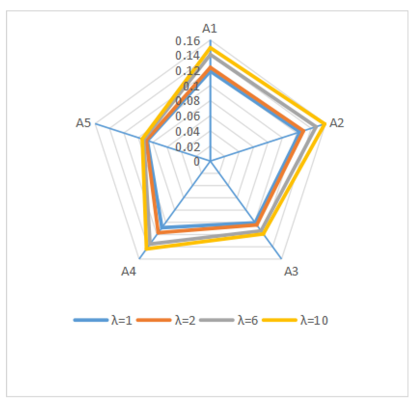
Thereafter, take $(\alpha ,\beta )$ as $(0.9,0.1)$, $(0.7,0.3)$, $(0.5,0.5)$, $(0.3,0.7)$, $(0.1,0.9)$, and take $\lambda =1,2,6,10$, respectively. By using Equation (20), the corresponding comprehensive deviations between each alternative and the ideal alternative are obtained, which are shown as

Table 2. Deviations between each alternative and the ideal alternative where $(\alpha ,\beta )=(0.9,0.1)$.

$\mathit{\lambda }$	${\mathit{A}}_1$	${\mathit{A}}_2$	${\mathit{A}}_3$	${\mathit{A}}_4$	${\mathit{A}}_5$	Ranking
$\lambda =1$	0.2612926	0.2612927	0.2631	0.2628	0.2582	$A_5\succ A_1\succ A_2\succ A_4\succ A_3$
$\lambda =2$	0.2622	0.2645	0.2636	0.2646	0.2585	$A_5\succ A_1\succ A_2\succ A_3\succ A_4$
$\lambda =6$	0.2661	0.2774	0.2656	0.2723	0.2593	$A_5\succ A_3\succ A_1\succ A_4\succ A_2$
$\lambda =10$	0.2699	0.2891	0.2672	0.2801	0.2602	$A_5\succ A_3\succ A_1\succ A_4\succ A_2$

,

Table 3. Deviations between each alternative and the ideal alternative where $(\alpha ,\beta )=(0.7,0.3)$.

$\mathit{\lambda }$	${\mathit{A}}_1$	${\mathit{A}}_2$	${\mathit{A}}_3$	${\mathit{A}}_4$	${\mathit{A}}_5$	Ranking
$\lambda =1$	0.2983	0.3021	0.2869	0.2904	0.2751	$A_5\succ A_3\succ A_4\succ A_1\succ A_2$
$\lambda =2$	0.3003	0.3054	0.2880	0.2940	0.2752	$A_5\succ A_3\succ A_4\succ A_1\succ A_2$
$\lambda =6$	0.3083	0.3186	0.2921	0.3073	0.2758	$A_5\succ A_3\succ A_4\succ A_1\succ A_2$
$\lambda =10$	0.3156	0.3304	0.2960	0.3178	0.2763	$A_5\succ A_3\succ A_1\succ A_4\succ A_2$

,

Table 4. Deviations between each alternative and the ideal alternative where $(\alpha ,\beta )=(0.5,0.5)$.

$\mathit{\lambda }$	${\mathit{A}}_1$	${\mathit{A}}_2$	${\mathit{A}}_3$	${\mathit{A}}_4$	${\mathit{A}}_5$	Ranking
$\lambda =1$	0.3409	0.3494	0.3143	0.3227	0.2944	$A_5\succ A_3\succ A_4\succ A_1\succ A_2$
$\lambda =2$	0.3445	0.3528	0.3173	0.3298	0.2958	$A_5\succ A_3\succ A_4\succ A_1\succ A_2$
$\lambda =6$	0.3588	0.3662	0.3274	0.3515	0.3002	$A_5\succ A_3\succ A_4\succ A_1\succ A_2$
$\lambda =10$	0.3707	0.3780	0.3347	0.3641	0.3032	$A_5\succ A_3\succ A_4\succ A_1\succ A_2$

,

Table 5. Deviations between each alternative and the ideal alternative where $(\alpha ,\beta )=(0.3,0.7)$.

$\mathit{\lambda }$	${\mathit{A}}_1$	${\mathit{A}}_2$	${\mathit{A}}_3$	${\mathit{A}}_4$	${\mathit{A}}_5$	Ranking
$\lambda =1$	0.3900	0.4041	0.3459	0.3604	0.3166	$A_5\succ A_3\succ A_4\succ A_1\succ A_2$
$\lambda =2$	0.3959	0.4076	0.3524	0.3729	0.3205	$A_5\succ A_3\succ A_4\succ A_1\succ A_2$
$\lambda =6$	0.4192	0.4211	0.3715	0.4051	0.3316	$A_5\succ A_3\succ A_4\succ A_1\succ A_2$
$\lambda =10$	0.4368	0.4329	0.3822	0.4197	0.3385	$A_5\succ A_3\succ A_4\succ A_2\succ A_1$

and

Table 6. Deviations between each alternative and the ideal alternative where $(\alpha ,\beta )=(0.1,0.9)$.

$\mathit{\lambda }$	${\mathit{A}}_1$	${\mathit{A}}_2$	${\mathit{A}}_3$	${\mathit{A}}_4$	${\mathit{A}}_5$	Ranking
$\lambda =1$	0.4465	0.4674	0.3823	0.4044	0.3418	$A_5\succ A_3\succ A_4\succ A_1\succ A_2$
$\lambda =2$	0.4559	0.4711	0.3941	0.4247	0.3497	$A_5\succ A_3\succ A_4\succ A_1\succ A_2$
$\lambda =6$	0.4914	0.4848	0.4250	0.4694	0.3702	$A_5\succ A_3\succ A_4\succ A_2\succ A_1$
$\lambda =10$	0.5157	0.4963	0.4390	0.4864	0.3833	$A_5\succ A_3\succ A_4\succ A_2\succ A_1$

.

Table 2, Table 3, Table 4, Table 5 and Table 6 show that the alternative ranking order varies when the parameters are valued differently. Therefore, decision makers with different subjective preferences can choose specific parameters according to their experiences and attitudes. It means that the proposed parameterized distance measures are beneficial for the combination of subjective and objective decision-making information.

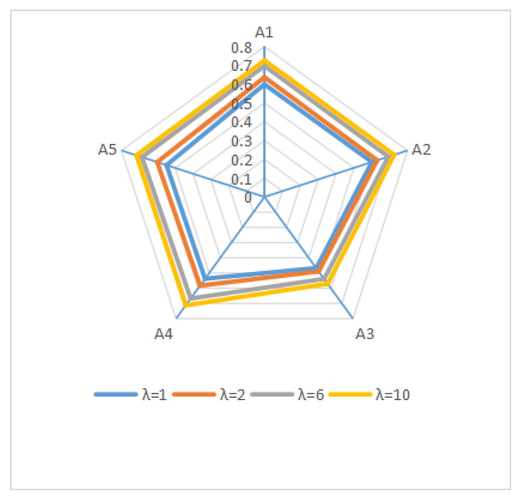
Moreover, the above results are not consistent with reference [18]. By using distance measures proposed in reference [18], the distances between each alternative and optimal alternative are obtained as Figure 2. In particular, the alternative ranking results are obtained as: (1) when $\lambda =1$, it gets $A_3\succ A_4\succ A_5\succ A_1\succ A_2$; (2) when $\lambda =2$, it gets $A_3\succ A_4\succ A_5\succ A_2\succ A_1$; (3) when $\lambda =6$, it gets $A_3\succ A_4\succ A_5\succ A_2\succ A_1$; and (4) when $\lambda =10$, it gets $A_3\succ A_4\succ A_5\succ A_2\succ A_1$.

Contrastive analysis shows that the distance from alternative $A_5$ and the ideal alternative varies greatly. By investigation, the reasons for this results are concluded as follows: (i) The element numbers of HFE $A_5$ is bigger than those of the other four HFEs. When distance measures proposed in reference [18] are used, the element numbers of HFEs are viewed as a part of the distance between them; therefore, the distance between $A_5$ and the ideal alternative is larger. ($ii$) In the newly proposed distance measures, the cardinality of HFE is transferred to credibility factor; therefore, the corresponding distance between $A_5$ and the ideal alternative is smaller. ($iii$) The distance measures proposed in reference [14] is suitable to weight the values in HFEs. When calculating the distance between $A_5$ and the optimal alternative, unduly large or small deviations on the aggregation results are assigned low weights. Therefore, the calculation results obtained by reference [14] and this study are consistent with each other.

In essence, the characteristic of the distance measures proposed in this study is that they can combine the subjective and objective information well. They are good complements to decision-making theory. This case also illustrates that the decision-making process is not a pure mathematical calculation, and decision makers should choose the most suitable distance measure according to the specific decision-making environment. This is also the reason why decision-making is fascinating.

5. Conclusions

In this study, the role of cardinality of HFE in distance measures on HFSs is analysed. Moreover, a series of parameterized distance measures on HFSs are proposed. The main innovation points of this study are as follows:

• In classical distance measures, the hesitance degree index of HFE is often calculated in addition to operations with the values of HFEs in classical distance measures. In contrast, the distance measures proposed in this study transfer the hesitance degree index to a credibility factor. Specifically, the credibility factor of HFE is calculated in multiplication operations with the values of HFEs in newly proposed distance measures, which handles the relationship between the cardinal number and the element values of hesitant fuzzy set well.
• In the newly proposed distance measures, there are three parameters. These parameters can be adjusted by decision makers according to the specific decision-making environment, which is beneficial for combining subjective and objective decision-making information, making the decision-making results more objective.

However, every method does have its limitations, and it is hoped that these novel distance measures could become perfect step-by-step in practice.