Utilizing Remotely Sensed Observations to Estimate the Urban Heat Island Effect at a Local Scale: Case Study of a University Campus

Abstract

The urban heat island (UHI) effect has become a significant focus of research in today’s era of climate change, and a key consideration for the next generation of urban planning focused on green and livable cities. UHI has traditionally been measured using in situ data and ground-based measurements. However, with the increased availability of satellite-based thermal observations of the Earth, remotely sensed observations are increasingly being utilized to estimate surface urban heat island (SUHI), using land surface temperature (LST) as a critical indicator, due to its spatial coverage. In this study, we estimated LST based on Landsat-8 observations to demonstrate the relationship between LST and the characteristics of the land use and land cover on the campus of King Abdulaziz University (KAU), Jeddah, Saudi Arabia. We found a consistent variation of between 7 and 9 degrees Celsius for LST across campus, spanning all summer and winter seasons between 2014 and 2019. The LST correlates strongly with both green vegetation and built-up land cover, with a slightly stronger correlation with the latter. The relationship between LST and green vegetation has a notable seasonality, with higher correlation in the summer seasons compared to the winter seasons. Our study also found an overall increase in LST between 2014 and 2019, due to intentional changes in the built-up land cover, for example from the conversion of natural green surfaces to artificial surfaces. The findings of this study highlight the utility of the remotely sensed observation of LST to assess the SUHI phenomenon and can be used to inform future planning aimed at securing green and livable urban areas in the face of a changing climate.

1. Introduction

Land surface temperature (LST), which is also referred to as the ‘surface radiometric temperature’ [1] or ‘radiative “skin” temperature’ [2], can be measured remotely, for example by satellite or airborne remote sensing. LST can be used to estimate radiation budgets and heat balance, and so can be used as a control for global climatological models [3]. LST is also a key factor when estimating the urban heat island (UHI) effect, i.e., when an urban area exhibits higher atmospheric and surface temperatures compared to adjacent rural areas [4], with a significant impact on the ecology, environment, and society [5]. In general, the UHI effect can be categorized into three main types: boundary layer urban heat island (BLUHI), canopy layer urban heat island (CLUHI) and surface urban heat island (SUHI) [6]. In this study, we examine the SUHI, as measured on the surface. Ensuring that cities are green and livable in the face of a changing climate requires careful consideration of the implications of SUHIs in urban planning [7]. Accurate and timely information regarding spatial and temporal variations in LST are essential for climatological, ecological, hydrological, and biogeochemical applications [8].

Patterns of land use and land cover (LULC) on Earth are essential factors affecting LST. Different LULC patterns are distinguished by unique reflectance and roughness, thereby leading to variations in LST [9,10]. Other factors, such as seasonality, climatological conditions [11], and the spatial clustering of the land cover [12], including its composition, configuration, complexity, intensity, morphology, and heterogeneity [3,13,14,15,16] are also key variables affecting LST.

Because LST is impacted by the characteristics of the land [17], LULC changes within urban areas and their fringes have a direct impact on LST [18,19]. In general, urban artificial impervious surfaces (roads, industrial areas, and other buildings) are associated with higher LST [20,21], compared to water bodies and vegetation land cover, which mitigate the microclimate conditions and lower the temperature in urban areas [22]. As a result, an increase in the area of asphalt roads and commercial and industrial land use, along with a decrease in the area of urban parks and gardens, other green spaces, and agricultural land is often associated with increased surface temperature [23], especially during the daytime [21]. Other factors affecting LST include, for example, building materials [10], the density of built-up structures, building heights, and population density [24]. Although the relationship between LST and the distribution of built-up land cover is not always linear and can vary by geography and seasonality [25], previous studies have found an association between LST and vegetation or built-up land cover, as measured utilizing remotely sensed observations; for example, using the normalized difference vegetation index (NDVI) and the normalized difference built-up index (NDBI) [26,27,28,29,30].

While previous studies have evaluated SUHI on the scale of a city or neighborhood, very few have measured and examined the SUHI effect on a local or micro scale by means of satellite observations. Many of the studies that examine micro-scale variations of UHI have used either in situ air measurements or airborne measurements at the surface level (e.g. [31,32]), with less emphasis on satellite-based observations.

Various micro-scale factors can potentially reduce the SUHI effect for local climate mitigation. For example, according to [33], SUHI can be eliminated when wind speed reaches a certain velocity, based on a “city-size-dependent threshold.” Similarly, an open low-rise gridiron precinct can potentially impact ventilation performance and, as a result, outdoor thermal comfort. According to [34], precinct ventilation performance has a clear positive impact in diminishing the SUHI effect by reducing humidity. When considered and implemented in urban planning, natural ventilation can often reduce the air temperature and enhance the subjective comfort experience [35,36]. A local climate zone (LCZ) relates to a classification system that aims to unify heat island measurement; LCZ was one of the first climate-based classifications for heat island studies [37]. The classification of the zones is not related to time, culture, or location, but it is quantifiable, based on land cover, building morphology, and thermal climate.

In light of the scarcity of studies that evaluate the relationship between LST and SUHI on a local scale, the main objective of this study was to examine the SUHI effect on a local scale, i.e., a university campus in Saudi Arabia. The study derived LST from publicly available Landsat-8 observations in the period 2013–2019, to identify and explain the relationship between LST and LULC. The analysis was implemented using the Google Earth Engine (GEE) (we provide a description about GEE in Section 2). This paper contributes to the existing body of literature by demonstrating the potential of Landsat-based observations to be used to estimate temporal trends in LST (annual and seasonal) at a local scale, and the relationship between these trends and changes in LULC characteristics. The study aimed to link LST and LULC to micro-scale planning decisions and show that Landsat-based measurements can be used to capture local and micro-scale changes in LST patterns.

2. Materials and Methods

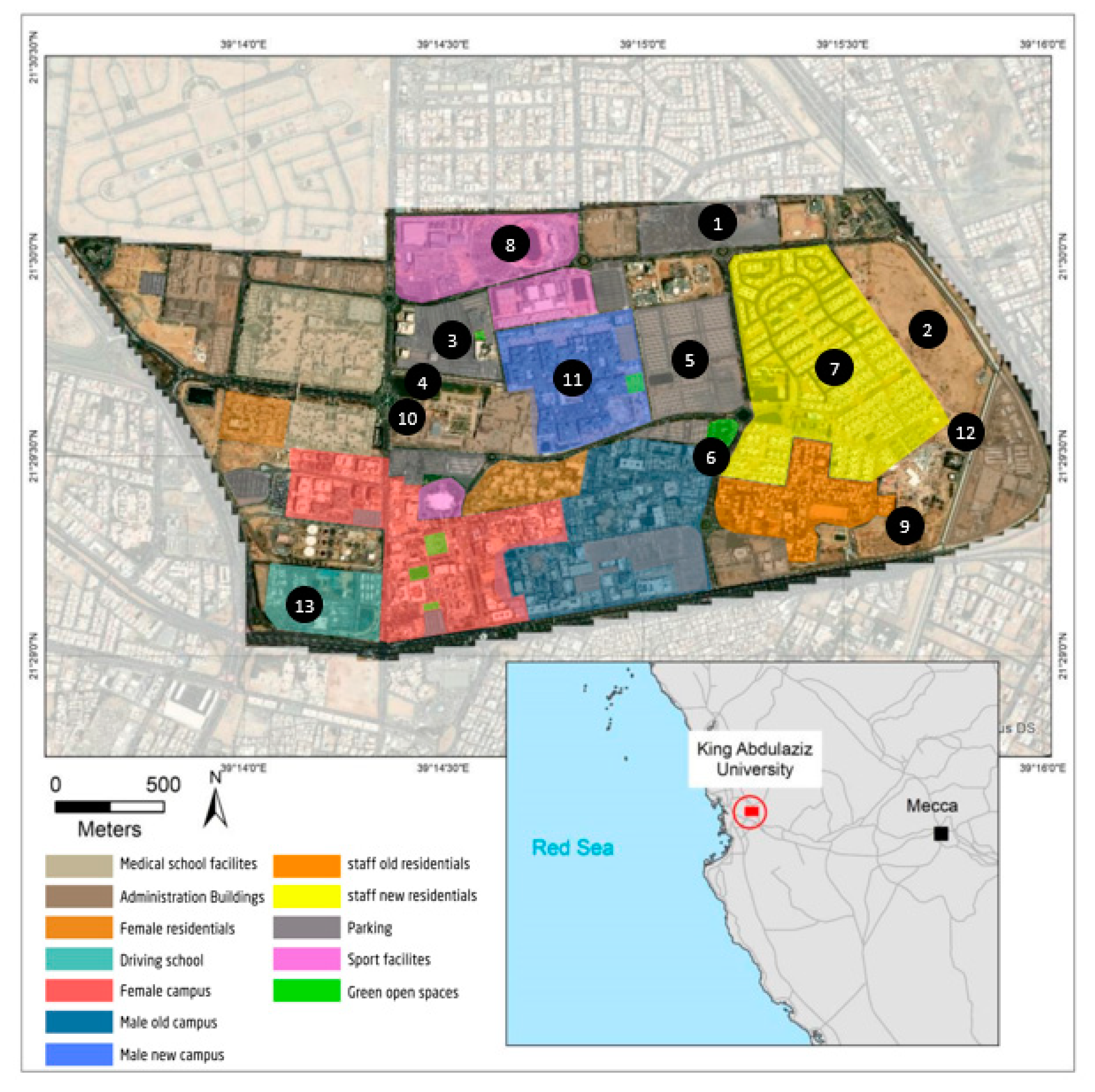
In this study, we analyzed the relationship between annual and seasonal variations in LST and changes in LULC in the King Abdulaziz University campus (KAU), between 2013 and 2019. We estimated and derived LST based on Landsat-8 observations (Tier 1 raw scenes). Furthermore, we estimate the characteristics of the land cover based on spectral indices. This is because the spectral indices prove to be an effective of mapping land cover [38] and provide better classification results [39]. In addition, it was derived from Landsat-8, as a proxy for vegetation land cover (NDVI), and for soil and built-up land cover ((NDBI) and Urban Index (UI)). Currently, there are two operating Landsat satellites, Landsat-7 (launched in 1999; carries the enhanced thematic mapper (ETM+) sensor) and Landsat-8 (launched in 2013; carries the operational land imager and TIRS camera). While both satellites can be used to derive LST, Landsat-8 has narrower spectral bands compared to Landsat 7, and TIRS provides additional capabilities for the estimation of LST compared to previous versions of Landsat. While previous studies have shown the potential of estimating LST from Landsat 7 data, some methods, such as the single-channel method which we used in this study, rely on Landsat-8’s B10 or B11 thermal bands.

We performed the analysis in Google Earth Engine (GEE), which is a platform that is frequently used for planetary-scale analysis in a wide range of applications [40], including mapping populations [41,42] and urban areas [43], as well as monitoring LULC changes and their relationship to SUHI [44,45].

2.1. Study Area

We evaluated the relationship between LST and land cover changes in KAU. Established in 1967, KAU occupies an area of 2224 acres (9 km²) in Jeddah, Saudi Arabia (between 21°29′N and 21°30′N latitude and 39°14′E and 39°16′E longitude). When KAU was established, the university buildings were constructed, primarily from natural stone, bricks, and concrete. The university campus has since grown, and new buildings have been constructed to expand faculties and accommodate more students. The newer buildings on campus often use granitic rock for decoration of the walls and floors [46]. The campus area includes faculty buildings, classrooms, the university hospital, sports facilities and the equestrian club, labs, central library, and administrative buildings and centers, as well as staff and female student housing. The campus has five public open spaces in the female campus and three in the male campus (Figure 1). These spaces account for 0.62% of the campus area. Furthermore, due to limited public transportation to serve the staff and students, there are many areas designated for car parking, which accounts for 10.42% of the campus area. (Figure 2 presents air photos of selected sites on campus. A detailed description of these sites and their characteristics is provided in Appendix A (

Table A1. Description of KAU sites, as presented in Figure 2.

	Area Description
1	It is located in the north of the University. Open area. Land cover is asphalt (parking area and the old driving school). Some parts include old and unused buildings and warehouses. It has some vegetation around the buildings.
2	It is located east of the campus. Open area. Land cover is compacted soil, and in the past, it was more natural, with natural vegetation. Currently, it has no vegetation or buildings.
3	It is located in the central part of the campus, toward the north. Parking space—not shaded. Only the parking close to the buildings is shaded with a tensile structure. Land cover is asphalt. From the east and the west, surrounded by administrative granite buildings and classrooms. There is no vegetation inside the area, but there are street trees in the north.
4	It is located in the central part of the campus, toward the west. Shaded and not shaded parking. Sports tent and female campus built with precast concrete buildings. Mature vegetation and lawn.
5	It is located in the center of the campus, toward the northeast. Shaded parking space. The shaded structure in the north part was completed in 2018. Land cover is asphalt. There are no buildings or vegetation inside the area.
6	It is located in the center of the campus, toward the east. Green space. Mature vegetation and lawn for the land cover and interlock tiles for the walkways.
7	It is located in the eastern part of the campus. Staff housing villas. It has open areas around mosques and pocket gardens. The building materials used for elevations are paint, due to the budget of the project. The building’s construction does not include green building approaches.
8	It is located in the northern part of the campus. Campus stadium and sports facilities. It includes the main stadium, small football fields and main gym buildings, made of granite and cladding. At the end of 2018, the natural turf was changed to artificial in the stadium and the football fields.
9	It is located in the southern part of the campus. Open area. Land cover is compacted land. It has scattered natural vegetation. The south of the area is Abdullah AlSuliman Street (main road). In the northwest border is the old staff housing made by precast concrete.
10	It is located in the central part of the campus, toward the northwest It is the main street to the higher administrivia buildings. The road edges and the roundabout have various types of vegetation.
11	It is located in the central part of the campus. The main academic and administrative buildings are made of granite. It has main unbuilt open spaces in the middle, which have very little natural vegetation. It has minimal vegetation in small areas (shrubs).
12	It is located in the southeastern part of the campus. Open area The land cover is natural land, with very little natural vegetation. It has warehouses and some construction waste.
13	It is located in the southwestern part of the campus. It is a female driving school, built in 2018. Until the end of 2017, it was a natural open area with native plants. The current land cover is asphalt with small buildings. It has no vegetation inside it, but there are mature trees from the west and the north.

)).

2.2. Data

2.2.1. Estimating LST

As with the methodology proposed by [47], we estimated LST based on Landsat-8 observations using a single-channel method, which has previously been shown to provide relatively accurate LST retrieval [48] and has been widely used due to its simplicity [49,50].

We relied on Band 10 (thermal infrared 1, resampled from 100 m to 30 m, 10.60–11.19 µm). Previous studies suggest that stray light artifacts due to out-of-field radiance that scatters onto the detectors are often found in TIRS data, adding a signal across the field-of-view that is non-uniform, and approximately twice as large in Band 11 as it is in Band 10 [48]. We estimated the average LST during the summer (21 June to 22 Sept) and the winter (22 Dec to 20 March) of each year between 2013 to 2019 (totaling 14-time intervals).

The procedure involves the following steps:

Identify Landsat scenes: We obtained Landsat 8 Collection 1 Tier 1 DN values, representing scaled, calibrated at-sensor radiance, which are available in GEE. Tier 1 includes Level-1 Precision Terrain (L1TP) processed data with well-defined radiometry, inter-calibrated across different Landsat sensors. We retrieved all Landsat-8 scenes that were captured during each time interval (we selected only scenes with less than 5% cloud coverage).

TOA spectral radiance: We converted the raw reflectance value in Band 10 (B10) of each scene into a TOA spectral radiance (radiance measured by the sensor). Two parameters are required to convert the DN value into TOA: the radiance multiplicative and the radiance add, which we extracted from the metadata of each scene using this expression:

$$TOA\left(L\right)=\left(ML\ast DN\right)+AL$$

(1)

where TOA (L) is the top of atmosphere radiance of B10, ML is the multiplicative rescaling factor of B10 in a given image, DN is the reflectance value of B10, and AL is the additive rescaling factor of B10 in a given image.

LST can be determined using the following expression:

$$LST=\gamma \ast \left[1/\epsilon \ast \left(\psi 1·Lsen+\psi 2\right)+\psi 3\right]+\delta$$

(2)

where ψ1, ψ2, and ψ3 can be derived as a function of total atmospheric water vapor content (w) using the following matrix approximation:

$$\left[\begin{array}{c}\psi 1\\ \psi 2\\ \psi 3\end{array}\right]=\left[\begin{array}{ccc}{C}_{11}& C_{12}& C_{13}\\ C_{21}& C_{22}& C_{23}\\ C_{31}& C_{32}& C_{33}\end{array}\right]\left[\begin{array}{c}w{v}^2\\ wv\\ 1\end{array}\right]$$

(3)

where w is the water vapor, and coefficients c_ij are derived from [47] as follows:

$$C=\left[\begin{array}{ccc}0.14714& -0.15583& 1.1234\\ -1.1836& -0.37607& -0.52894\\ -0.04554& 1.8719& -0.39071\end{array}\right]$$

(4)

We retrieved water vapor content information from NCEP/NCAR. The NCEP/NCAR Reanalysis Project is a joint initiative between the National Centers for Environmental Prediction (NCEP, formerly NMC) and the National Center for Atmospheric Research (NCAR). The goal of the project is to produce atmospheric analyses based on historical data, along with analyses of the current atmospheric state (climate data assimilation system, CDAS) (also available in GEE). We retrieved surface water vapor information for the corresponding date of each Landsat scene (four observations per day) and calculated the average water vapor over the four observations per day. We calculated emissivity (ε) according to the following expression [47]:

$$\epsilon ={\epsilon }_{nonveg}\ast \left(1-FVC\right)+{\epsilon }_{veg}\ast FVC$$

(5)

where fractional vegetation cover (FVC) is calculated as:

$$FVC=\left[\left(NDVI-NDV{I}_{min}\right)/\left(NDV{I}_{max}+NDV{I}_{min}\right)\right]^2$$

(6)

Moreover, $\epsilon$ is the surface emissivity of vegetated (${\epsilon }_{veg}$) and soil (${\epsilon }_{nonveg}$). surfaces. Like [51], we assumed soil and vegetation emissivities of 0.97 and 0.99, respectively.

Finally, we converted the LST values in Kelvin to degrees Celsius. We estimated the LST for each pixel in each Landsat scene over each interval (season) and calculated per pixel, per season LST values as the average value of all overlapping pixels in an interval. As explained above, the main objective of this study was to estimate seasonal variations in LST and their relationship to LULC changes. In this respect, it should be mentioned that, while LST, by its nature, may fluctuate due to microclimate conditions, the characteristics of LULC do not tend to change much monthly. While some previous studies have examined the relationship between temperature and LULC by using single daily images [52], other studies have captured long-term variations using monthly, seasonal [53] or annual composites [54]. In this research, we examined seasonal and annual variations in LST, rather than daily or bi-weekly trends. This method aims to capture broad seasonal trends in LST and LULC (estimated as the average across an entire season), rather than to examine daily climatological trends that are less related to LULC patterns.

2.2.2. LULC Characteristics

To establish the relationship between LST and the characteristics of land cover, we relied on several remote-sensor-derived spectral indices, which we obtained from Landsat-8 Collection 1 Tier 1 calibrated TOA reflectance composites (available in GEE).

NDVI: NDVI [55] conveys the relationship between visible red light (which is absorbed by chlorophyll) and near-infrared wavelength (which is scattered by leaf mesophyll cells). It is calculated as:

$$\frac{\left(NIR-RED\right)}{\left(NIR+RED\right)}$$

(7)

where NIR is the near-infrared wavelength, and the RED is the red wavelength (Bands 5 and 4, respectively, in Landsat 8). NDVI ranges from (−1) to (+1). An NDVI value was calculated for each pixel per season (average value for all overlapping pixels in scenes with less the 25% cloud coverage during a season).

NDBI: NDBI [56] conveys the relationship between medium infrared and near-infrared wavelengths. It is calculated as:

$$\frac{\left(SWIR1-NIR\right)}{\left(SWIR1+NIR\right)}$$

(8)

where SWIR1 is the reflectance in the shortwave infrared wavelength (1.57– 1.65 µm), and NIR is the reflectance in the near-infrared wavelength (Bands 6 and 5, respectively, in Landsat 8). NDBI ranges from (−1) to (+1). An NDBI value was calculated for each pixel per season (average value for all overlapping pixels in all scenes with less the 25% cloud coverage during a season).

UI: UI [57] normalizes the NIR and SWIR 2 bands (Bands 7 and 5 in Landsat 8) and relies on the inverse relationship between the brightness of the NIR and SWIR in built-up areas. Previous studies have used UI to measure urbanization and urban sprawl [58] and to extract the extent of built-up land cover from remotely sensed observations [59]. The index is calculated as follows:

$$\frac{\left(SWIR2-NIR\right)}{\left(SWIR2+NIR\right)}$$

(9)

A UI value is calculated for each pixel per season (average value for all overlapping pixels in scenes with less than 25% cloud coverage during a season).

2.2.3. Aggregation to the Hexagon Level and Analysis

• Aggregation to the hexagon unit of analysis (hexagonal tessellation)

For this study, we used a hexagon tessellation mapping procedure to estimate the relationship between patterns of LST and LULC. Aggregating pixel-level data to a given unit of analysis is necessary when analyzing LULC characteristics at different geographical scales. The approach of relying on hexagonal tessellation for LULC research, which can also be referred to as ‘zone mapping’ [60], has previously been used in the remote sensing domain [61,62]. It allows the creation of areas that are relatively homogenous in terms of their land cover and land use spectral reflectance, as well as their LST. Here, we created a grid of cells (hexagonal tessellation) of 2546 hexagons that span the campus; each hexagon is around 3100 m² (compared to an approximate area of a Landsat pixel being 900 m², i.e., around 3–4 Landsat pixels overlapping with one hexagon). For each hexagon, we calculated the average LST, NDVI, NDBI, and UI values of each overlapping pixel.

• Correlation and multiple regression analysis

We relied on the hexagons in the hexagonal tessellation as the units of analysis. We evaluated the correlation (Spearman correlation test) between LST and each of the indices. In addition, we calculated the per-hexagon slope of change (SOC) of LST, NDVI, NDBI, and UI values over the period 2014 to 2019 (we define SOC as the rate of change or slope of a linear function between LST and the spectral indices). Furthermore, we performed a multiple regression analysis to estimate the potential of the explanatory variables to explain, together, variations in LST. Multiple regression analysis has previously been used in the field of remote sensing research; for example, by [63], who estimated the potential of 28 remotely sensed derived variables to explain variations in air temperature, or by [64], who performed a thermal unmixing approach, calculated using multiple linear regression to evaluate the relation between LULC patterns and LST.

• Getis-Ord Gi* for hot spot analysis

We also evaluated changes in patterns of LST and patterns of LULC using the Getis-Ord Gi*method for hot spot analysis [65]. This method is ideal for identifying local patterns in the spatial distribution of data, which could not have been revealed using global statistical measures [65]. In other words, because global statistics conducted over an entire area of interest are often too coarse and are insensitive to local “nuances,” the Getis-Ord Gi* method was used to locate and identify clusters of concentration of high or low values [66]. Given a set of weighted features, Getis-Ord Gi* statistics identify statistically hot and cold spots. Here, we calculated the Getis-Ord Gi* statistic for each hexagon in the dataset, which allowed us to identify hexagons that exhibit high and low values that are spatially clustered. The Getis-Ord Gi* statistic is calculated as [67]:

$$G_i^{*}=\frac{{{\displaystyle \sum }}_{j=1}^n{w}_{i,j}{x}_j-\overline{X}{{\displaystyle \sum }}_{j=1}^n{w}_{i,j}}{\sqrt[s]{\frac{\left[n{{\displaystyle \sum }}_{j=1}^n{w}_{i,j}^2-{({{\displaystyle \sum }}_{j=1}^n{w}_{i,j})}^2\right]}{n-1}}}$$

(10)

where $x_j$ is an attribute value of feature j, $w_{i,j}$ represents a spatial weight between feature i and j, while n is the number of features, and:

$$\overline{X}=\frac{{{\displaystyle \sum }}_{j=1}^n{x}_j}{n}$$

(11)

$$S=\sqrt{\frac{{{\displaystyle \sum }}_{j=1}^n{x}_j^2}{n}-{\left(\overline{X}\right)}^2}$$

(12)

3. Results

This section is divided into four sub-sections. First, we present the spatial and temporal patterns of LST. Then, we present a detailed analysis of the relationship between spatial and temporal patterns of LST and LULC, along with the results of correlation and regression tests to estimate the relationship between changes in LST and changes in LULC. Finally, we present the results of the Getis-Ord Gi* hot spot analysis, to identify temporal changes in hot and cold spots of LST and LULC.

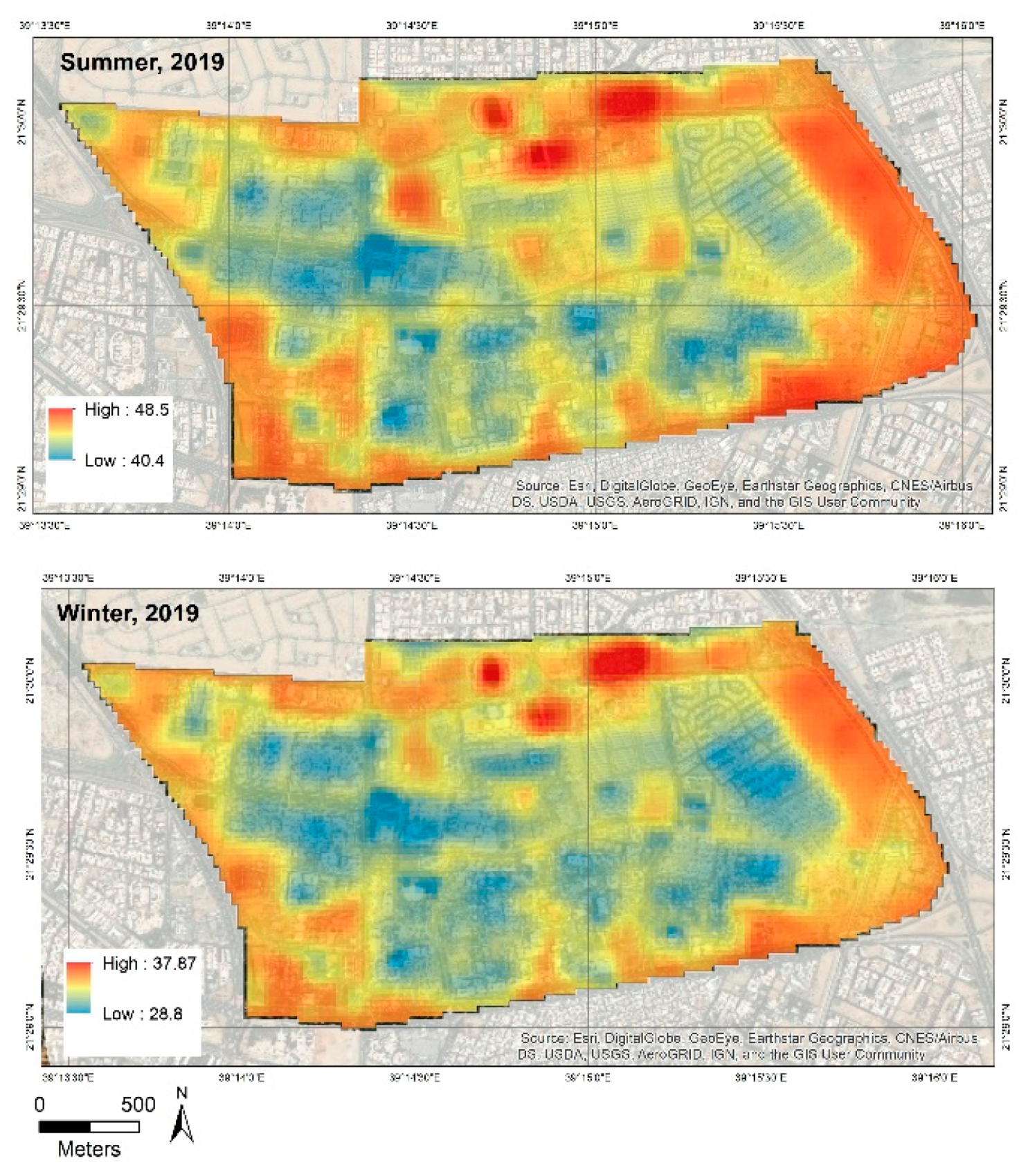
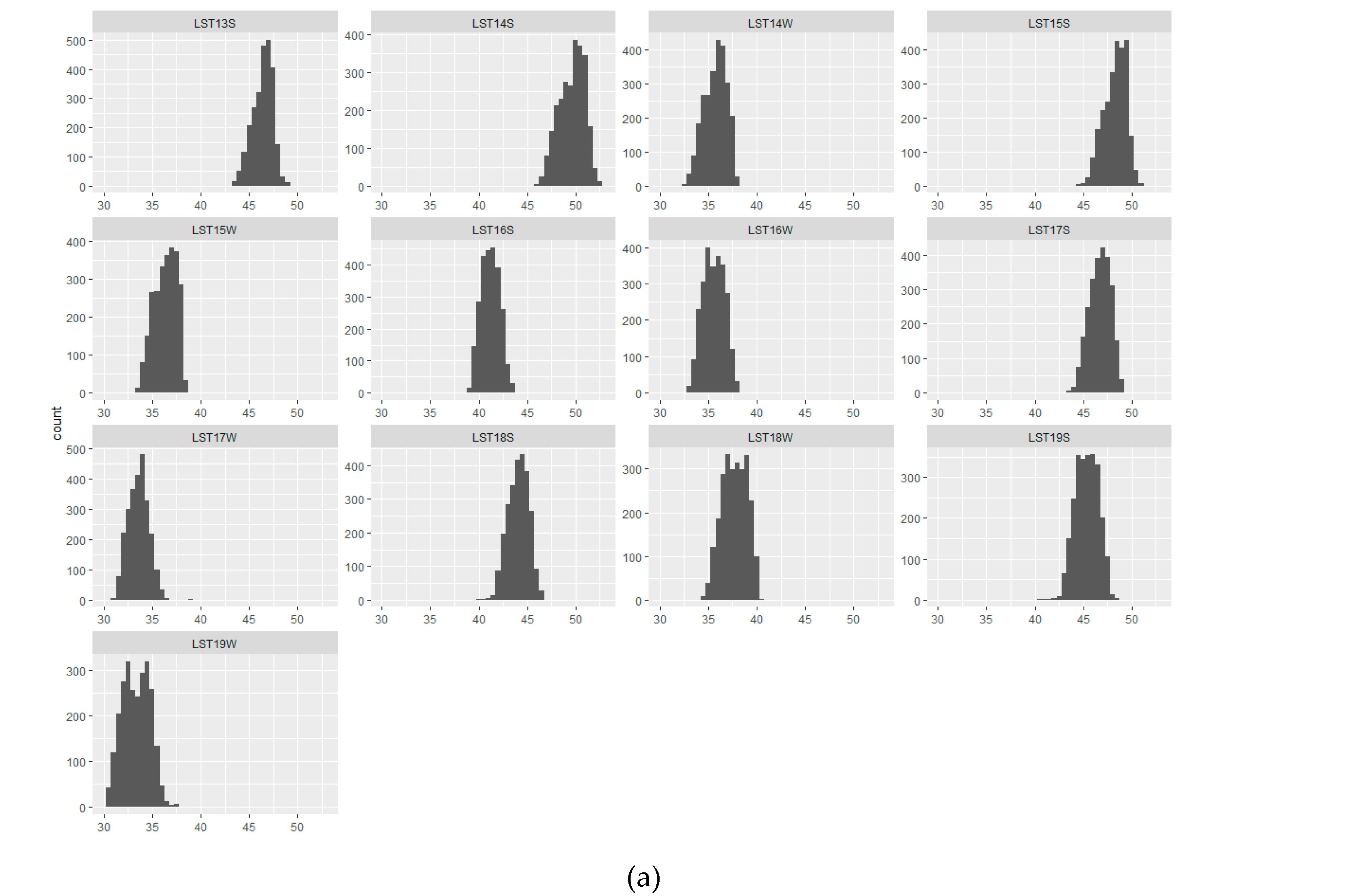
3.1. Spatial and Temporal Patterns of LST

The analysis shows clear spatial and temporal variations in the distribution of the LST across the KAU campus. As can be seen in Figure 3 (seasonal trends in average LST in the period between 2013 and 2019), the average remotely sensed, derived seasonal LST ranged between 45.96 °C (Std = 2.57 °C) in the summer, and 35.39 °C (Std = 1.53 °C) in the winter. The highest summer temperature was recorded in 2014, and the highest winter temperature was recorded in 2018. In addition, we find a clear variation in the spatial distribution of LST across campus. Figure 4 presents, as an illustration, the distribution of LST in the summer and winter of 2019. In summer 2019, the LST ranged between 48.5 °C and 40.4 °C. In the winter of 2019, LST ranged between 37.87 °C and 28.7 °C. The results suggest some similarities between summer and winter in the distribution of the LST.

In general, we find that open spaces that are not covered with green vegetation (typically, bare land or other types of surface, such as asphalt and compressed soil) are characterized by a relatively high LST. This trend is observed, for example, over the open areas in the northern part of campus (area number 1, Figure 2), and east to the staff housing (area number 2, Figure 2), as well as over several paved parking spaces (e.g., areas number 3, Figure 2). For example, in summer 2019, the temperature over the main campus parking lot (area number 3, Figure 2) was 6.5 °C higher than over the green space south of the parking lot (area number 4, Figure 2) (i.e., 47.18 °C compared to 40.72 °C, respectively) (the distance between these areas is approximately 250 meters). Due to a lack of public transportation within the campus and between the campus and Jeddah and surrounding cities, there are many parking spaces (e.g., areas number 3 and 5, Figure 2), most of which are not proximal to trees or shading structures. The LST over these parking spaces is up to 6 °C higher, compared to the temperature over adjacent green spaces across campus. Some of the cooler areas on campus include the space near the sports tent (area number 4, Figure 2), the park in the central-eastern part of the campus (which is characterized by mature trees and various planting types) (area number 3, Figure 2), and even the shaded parking space west of the staff housing (area number 5, Figure 2). These trends are also evident in the winter. In winter 2019, the temperature over the parking spaces across campus was around 34.5 °C (areas number 3 and 5, Figure 2), compared to the temperature over the green spaces, which was approximately 30.7 °C (areas number 6 and 4, Figure 2).

Study area number 7, which is new staff housing at the University, shows a consistently low LST, both in winter and in summer. A potential explanation for this result could be the white-painted roof of staff housing, which is a rarity on the KAU campus and the orientation of the buildings. These buildings are structures on a 45°-degree angle to the direction of the wind, which enhances natural ventilation. In addition, the form of the buildings and the staggered layout help in accentuating the wind movement between blocks. Hence, the orientation of the buildings, which allows for wind movement and increased velocity, together with the painted roof, may explain, at least in part, the lower LST observed over Area 7 (staff housing).

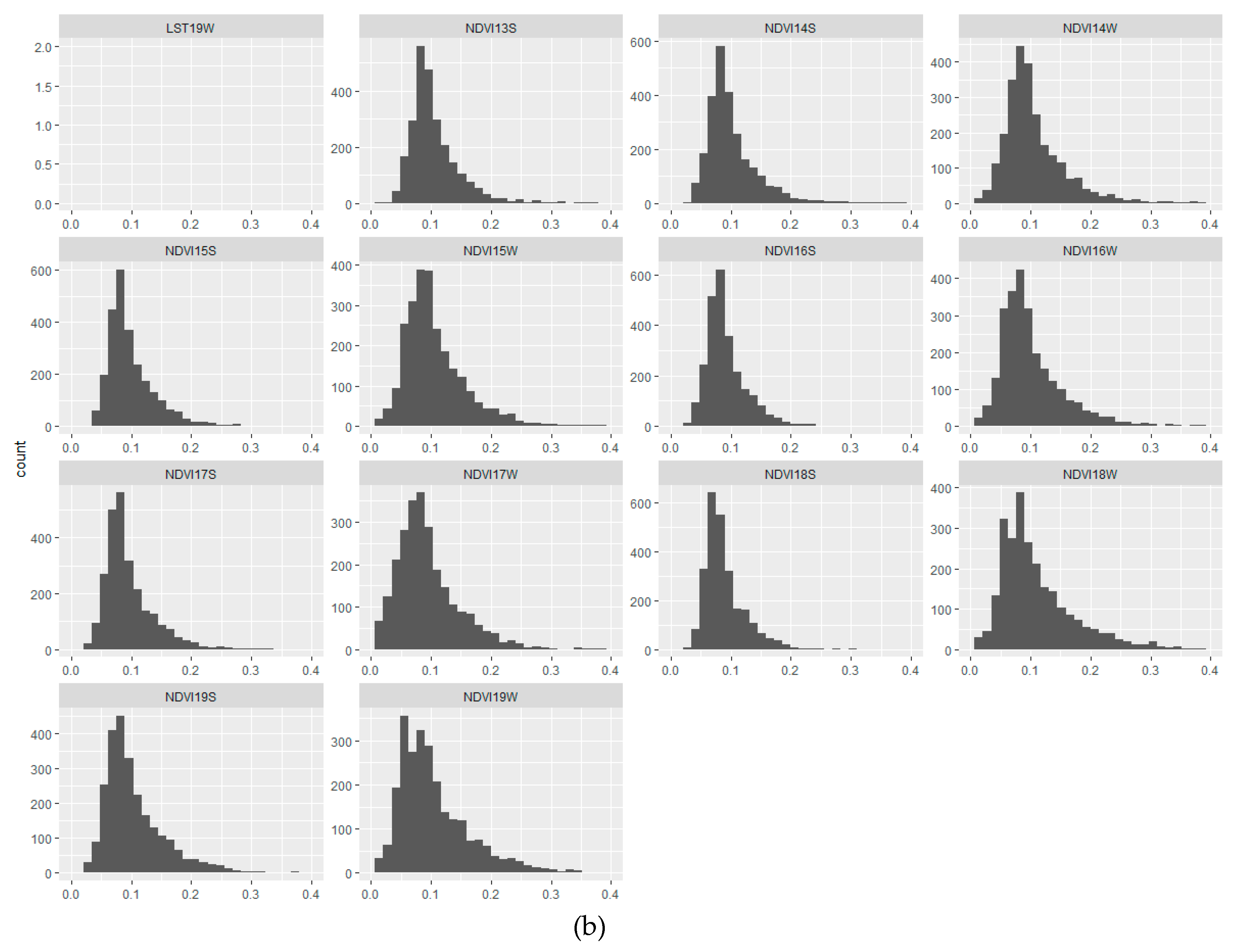
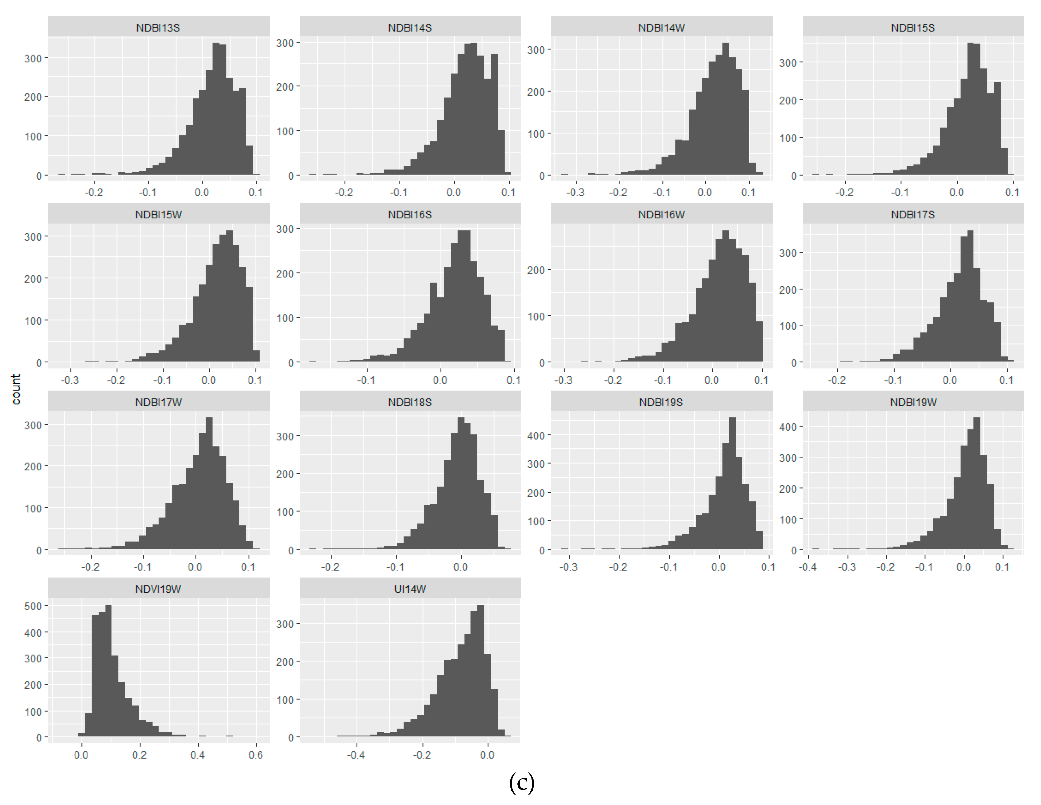
3.2. The Relation between Patterns of LST and LULC

The spatial variations in LST can be explained, at least partly, by the distribution of green vegetation across the campus. To identify the relationship between the distribution of green vegetation and built-up land cover with LST, we overlaid hexagons with the highest NDVI and NDBI values (i.e., hexagons with an average NDVI and NDBI values that exceeded a set threshold, which we defined as the 80th percentile of the NDVI and NDBI value of all hexagons in the dataset). Figure 5 presents, as an illustration, the hexagons that exhibit the highest NDVI and NDBI values in the winter and summer of 2019, against LST (these hexagons are characterized by an NDVI value that is greater than 0.115 and 0.136 and with an NDBI value greater than 0.049 and 0.043 for the winter and summer, respectively). As clearly illustrated in Figure 5, hexagons that exhibit the highest NDVI value are also characterized by relatively low temperatures, while hexagons that exhibit high NDBI are characterized by higher temperatures. This trend is observed in the winter and the summer. In other words, higher LST corresponds with less green vegetation and more built-up land cover.

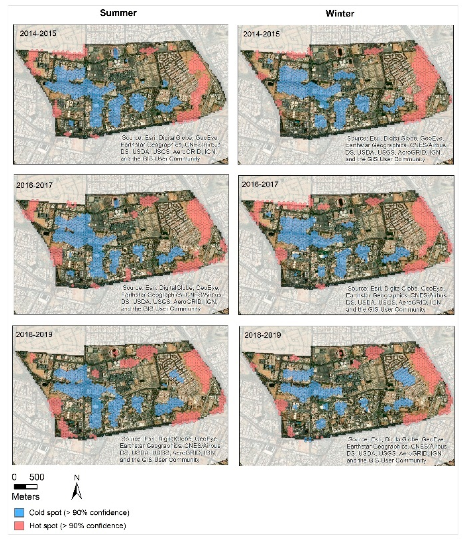
3.3. Getis-Ord Gi* Hot Spot Analysis

To identify temporal trends in LST, we performed hot spot analysis using Getis-Ord Gi* [65], which allows the estimation of hot and cold spots by examining features and their neighbors. For example, a feature (hexagon) is characterized as a statistically hot spot if both it and other surrounding features (hexagons) have high values [25]. Because the correlation and regression tests are performed at the geographical unit of the hexagon, we also perform the Getis-Ord Gi* at the hexagonal unit. This allows us to estimate the extent to which the observed changes in the correlations between the variables are also reflected in their spatial patterns. We calculated the average temperature in the summers and winters of 2014–2015, 2016–2017, and 2018–2019, and identified significantly hot and cold spots based on Getis-Ord Gi* analysis (we choose to calculate the average over two-year intervals to identify changes in the patterns over the time visually). We found changes in the spatial patterns of LST across the campus, which we related to changes in LULC. For example, the campus stadium (area number 8, Figure 2) changed from a cold spot (in 2014–2015 and 2016–2017) to a hot spot (in 2018–2019). We linked this to changes in the stadium’s field ground from natural to artificial turf (in 2018, all sports grounds on campus were changed to artificial turf to reduce maintenance and irrigation costs), which has probably resulted in a significant increase in the LST. Another example can be found in the southwestern part of the campus (the driving school, area number 13, Figure 2). Until the end of 2017, this area was an open empty ground, covered with green vegetation (native plants) and designated for future development. At the beginning of 2018, this area was developed to become the University’s driving school. While this area does not have many structures, it incorporates a large asphalt surface for parking and driving practice. This new development resulted in this area becoming a hot spot in 2018–2019. Some new cold spots in 2018–2019 were found around the staff housing in the east part of the campus (area number 7, Figure 2), and are probably the result of the implementation of green open spaces upon the completion of the construction project in 2019.

To evaluate the relationship between changes in LST and changes in LULC, we calculated hot and cold spots for built-up land cover (NDBI and UI) and green vegetation (NDVI) (we used Getis-Ord Gi*). As can be seen in Figure 6 (hot and cold spots of live vegetation), several changes can be observed across time in the patterns of green vegetation (i.e., areas that exhibit significantly high NDVI values). In 2018–2019, for example, there were some new hot spots of green vegetation along the main street and entrance to the Higher Management Building (area number 10, Figure 2), which are likely to be the result of incorporating new green vegetation and natural turf. Several hot spots of built-up land cover (measured according to NDBI) can be seen, especially along the eastern and southern boundaries of the campus. A significant hot spot of built-up land cover can be seen around the academic square, or the new male campus, which is located at the center area of the campus (area number 11, Figure 2). This area incorporates large faculty and administration buildings and has little green vegetation. This area is also a hot spot with high LST (Figure 7). Changes in the observed spatial patterns of built-up areas (according to NDBI) in the period between 2014 and 2019 can be seen in the area surrounding the staff housing (area number 12, Figure 2), which was a hot spot of high NDBI in 2014–2015 (the construction of this area was completed at the end of 2018) (Figure 8). In parallel with the change of this area from a hot spot of NDBI to a non-hot spot, this area became a cold spot for LST. Additionally, in 2014–2015, the area in the southern part of the campus (area number 13, Figure 2) used to be a cold spot of NDBI. This area was constructed in 2018. As a result, this area showed an increase in LST between 2014–2015 and 2018–2019, causing it to change gradually from a cold spot of LST to a non-cold spot.

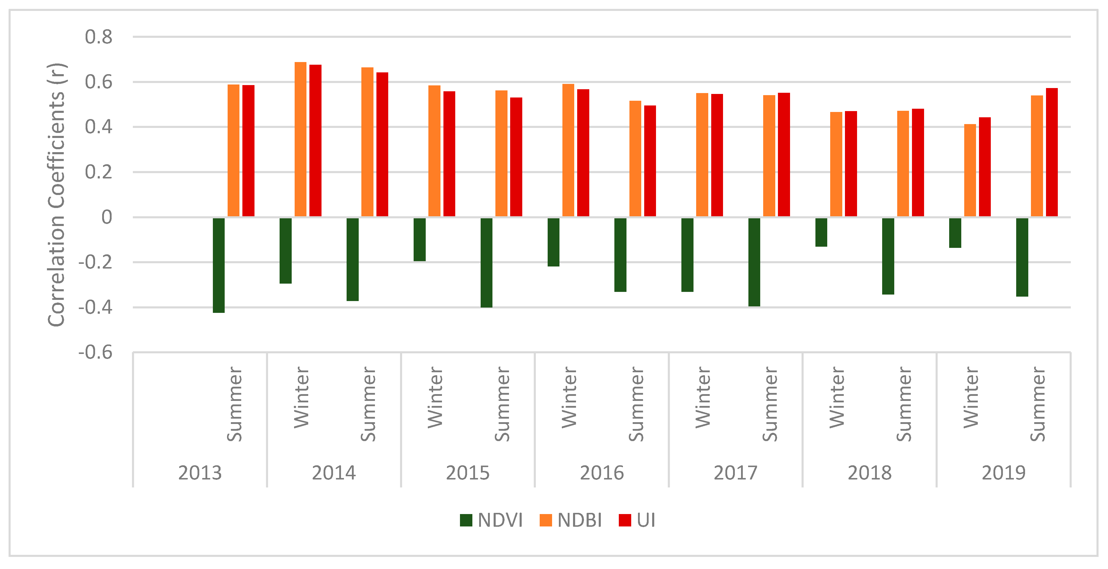
3.4. LST and LULC Correlation and Regression Tests

To further evaluate the relationship between LST and the patterns of LULC, we performed a correlation test to estimate the correlation between green vegetation (NDVI) and built-up land cover (NDBI and UI) and LST. We provide, in Appendix A (Figure A1), as an illustration, the distributions (histograms) of LST, NDVI and NDBI values across all the hexagons in the study area. As can be observed, the values are not normally distributed and are skewed either to the right (NDVI) or left (NDBI). A Shapiro–Wilk normality test confirmed that the values are not normally distributed (

Table 1. Shapiro–Wilk test for normality. Examination of the distribution of LST, NDVI, NDBI, and UI during the summer and winter (2013–2019).

	Summer
	LST
	2013	2014	2015	2016	2017	2018	2019
W	0.98415	0.97712	0.97977	0.99088	0.98885	0.99146	0.99125
p-value	0.000	0.000	0.000	0.000	0.000	0.000	0.000
	NDVI
W	0.84757	0.83903	0.84063	0.8825	0.86209	0.86565	0.86902
p-value	0.000	0.000	0.000	0.000	0.000	0.000	0.000
	NDBI
W	0.93511	0.93776	0.92624	0.95469	0.9552	0.95504	0.91619
p-value	0.000	0.000	0.000	0.000	0.000	0.000	0.000
	UI
W	0.93363	0.93168	0.92503	0.93798	0.94714	0.93924	0.91778
p-value	0.000	0.000	0.000	0.000	0.000	0.000	0.000
	Winter
	LST
	2013	2014	2015	2016	2017	2018	2019
W		0.98003	0.97472	0.98669	0.99127	0.97977	0.76887
p-value		0.000	0.000	0.000	0.000	0.000	0.000
	NDVI
W		0.84543	0.87519	0.86753	0.9208	0.87598	0.85601
p-value		0.000	0.000	0.000	0.000	0.000	0.000
	NDBI
W		0.93954	0.93541	0.94447	0.95796	0.93837	0.91166
p-value		0.000	0.000	0.000	0.000	0.000	0.000
	Urban Index (UI)
W		0.92928	0.93733	0.94189	0.95279	0.9403	0.91984
p-value		0.000	0.000	0.000	0.000	0.000	0.000

presents the results of the test, indicating a p-value of 0, i.e., the test rejects the hypothesis of a normal distribution). While the Pearson Correlation test measures the linear relationship between two variables, the Spearman rank-order test measures the rank order of two variables and is a nonparametric version of the Pearson test. Spearman’s test may be more appropriate than the Pearson test, especially when the variables are characterized by a high kurtosis and can be used to determine if there is an association between two nonparametric variables. Here, we performed a Spearman’s rank-difference coefficient test to estimate the relationship (correlation) between the variables.

We calculated this correlation for each time interval (season) (Figure 9). The results show a significant and positive correlation between LST, NDBI, and UI (up to r = 0.69 and r = 0.68, respectively, p < 0.001 for both), in parallel to a significant negative correlation between NDVI and LST (up to r = −0.43, p < 0.001). These results suggest that LST is negatively correlated with green vegetation and positively correlated with built-up land cover. Interestingly, while the correlation between LST, NDBI, and UI does not vary much by season, the correlation between LST and NDVI does vary by season, with a stronger (negative) correlation in the summer compared to the winter (indicated by a correlation of up to r = −0.42 in the summer and up to r = −0.33 in the winter; p < 0.001 for both). These results imply that, first, LST is more impacted by the distribution of built-up land cover on campus than by the distribution of vegetation, and second, that the effect of vegetation on moderating the temperature is more significant in the summer than in the winter.

Next, to evaluate the explanatory power of the spectral indices to predict LST, we performed a multiple regression analysis. The results (presented in

Table 2. Multiple regression analysis to estimate the potential of the three examined spectral indices (NDVI, NDBI, and UI), to predict LST in the summer and the winter seasons of 2013–2019.

	Summer
	2013	2014	2015	2016	2017	2018	2019
NDVI	R2 = 0.2445 *	R2 = 0.1946 *	R2 = 0.233 *	R2 = 0.1513 *	R2 = 0.2303 *	R2 = 0.1867 *	R2 = 0.1901 *
	F(1,2544) = 824.6	F(1,2544) = 615.9	F(1,2544) = 774.3	F(1,2544) = 454.9	F(1,2544) = 762.4	F(1,2544) = 585.1	F(1,2544) = 598.4
	RMSE = 0.895	RMSE = 1.162	RMSE = 1.002	RMSE = 0.876	RMSE = 0.954	RMSE = 0.960	RMSE = 1.064
NDVI + NDBI	R2 = 0.3704 *	R2 = 0.439 *	R2 = 0.3512 *	R2 = 0.2819 *	R2 = 0.338 *	R2 = 0.2675 *	R2 = 0.3093 *
	F(1,2543) = 749.7	F(1,2543) = 996.7	F(1,2543) = 689.9	F(1,2543) = 500.6	F(1,2543) = 650.7	F(1,2543) = 465.8	F(1,2543) = 570.8
	RMSE = 0.817	RMSE = 0.970	RMSE = 0.922	RMSE = 0.806	RMSE = 0.885	RMSE = 0.911	RMSE = 0.983
NDVI + NDBI + UI	R2 = 0.3746 *	R2 = 0.4468 *	R2 = 0.3511 *	R2 = 0.2817 *	R2 = 0.3414 *	R2 = 0.2795 *	R2 = 0.3506 *
	F(1,2542) = 509	F(1,2542) = 686	F(1,2542) = 459.9	F(1,2542) = 333.7	F(1,2542) = 440.7	F(1,2542) = 330	F(1,2542) = 459.1
	RMSE = 0.814	RMSE = 0.963	RMSE = 0.922	RMSE = 0.806	RMSE = 0.883	RMSE = 0.904	RMSE = 0.953
	Winter
NDVI	-	R2 = 0.1168 *	R2 = 0.0715 *	R2 = 0.0856 *	R2 = 0.1352 *	R2 = 0.0466 *	R2 = 0.0356 *
		F(1,2544) = 337.6	F(1,2544) = 197.1	F(1,2544) = 239.2	F(1,2544) = 399	F(1,2544) = 125.4	F(1,2544) = 94.93
		RMSE = 1.081	RMSE = 1.105	RMSE = 1.05	RMSE = 0.970	RMSE = 1.240	RMSE = 1.658
NDVI + NDBI	-	R2 = 0.4675 *	R2 = 0.3838 *	R2 = 0.3757 *	R2 = 0.2953 *	R2 = 0.2909 *	R2 = 0.1428 *
		F(1,2543) = 1118	F(1,2543) = 793.6	F(1,2543) = 766.8	F(1,2543) = 534.3	F(1,2543) = 523.1	F(1,2543) = 213.1
		RMSE = 0.837	RMSE = 0.899	RMSE = 0.865	RMSE = 0.876	RMSE = 1.072	RMSE = 1.563
NDVI + NDBI + UI	-	R2 = 0.4868 *	R2 = 0.3994 *	R2 = 0.3816 *	R2 = 0.2981 *	R2 = 0.3168 *	R2 = 0.1735 *
		F(1,2542) = 805.7	F(1,2542) = 565.1	F(1,2542) = 524.4	F(1,2542) = 361.4	F(1,2542) = 394.3	F(1,2542) = 179.1
		RMSE = 0.822	RMSE = 0.888	RMSE = 0.861	RMSE = 0.874	RMSE = 1.053	RMSE = 1.534

Note: * p < 0.01.

) show that, together, NDVI, NDBI, and UI explain up to 49% of the variation in LST (in winter, 2014). In all seasons examined, we found that the explanatory power of NDVI is relatively low (up to R² = 24% in summer, 2013), and that it is lower in the summer than in the winter. We also found that the addition of NDBI and UI as additional explanatory variables improves the prediction, in which there is much less variation between winter and summer.

Finally, to evaluate the relationship between temporal changes in LST and LULC (namely, green vegetation and built-up land cover), we performed a Spearman correlation test to (

Table 3. Spearman correlation test of the correlation between changes in LST, NDVI, NDBI, and UI: absolute difference (Difference) and SOC between 2014 and 2019.

From	To		NDVI	NDBI	UI
(average)	(average)		Summer
2014–2015	2016–2017	Difference	−0.32 *	0.26 *	0.24 *
2016–2017	2018–2019	Difference	−0.03 **	0.31 *	0.35 *
2014–2015	2018–2019	Difference	−0.11 *	0.34 *	0.37 *
		SOC	−0.10 *	0.3 *	0.32 *
			Winter
2014–2015	2016–2017	Difference	-	0.36 *	0.330 *
2016–2017	2018–2019	Difference	0.05 **	0.13 *	0.21 *
2014–2015	2018–2019	Difference	-	0.29 *	0.32 *
		SOC	0.01 *	0.32 *	0.35 *

Note: * p < 0.01, ** p < 0.1.

) estimate the correlation between changes (absolute difference) in LST, NDVI, NDBI, and UI and between the SOC of the values over the period 2014 to 2019 (we define SOC as the rate of change or slope of a linear function between LST and the spectral indices). The results show a significant positive correlation, primarily between changes in LST and changes in built-up land cover (NDBI, UI) (up to r = 0.37 for changes in UI and LST between 2014–2015 and 2018–2019). The correlation is much weaker when examining the relationship between changes in LST and green vegetation (NDVI) (we only found a correlation for changes in LST and NDVI between the summer of 2014–2015 and 2016–2017 (r = −0.32)). We found a correlation between the SOC of LST and the SOC of NDBI and UI, both in the winter and in the summer (r = 0.32 and r = 0.35 for the correlation between the SOC in LST and UI during the winter and the summer seasons in the period between 2014 and 2019), indicating that the faster the change in UI values, the faster the changes in LST.

4. Discussion

The SUHI effect, i.e., when an urban area exhibits a higher atmospheric and surface temperature than adjacent rural areas [4], has been the subject of a large body of studies. Many factors affect the extent and nature of SUHI, including LULC characteristics [68] and their spatial patterns and configuration [17]. Changes in the characteristics of LULC, including the extent of impervious surfaces and built-up structures, have implications for the local and regional-scale climate, including on the SUHI [17,25,69,70]. Because green spaces and vegetation can mitigate the impact of the SUHI [71] effect and decrease the temperature [72,73], urban university campuses, which often have large areas of vegetation and green space, play a valuable role in mitigating the SUHI effect and helping to reduce its negative impact [74].

Until recently, the SUHI studies mainly use three type of data: in situ temperature observation, remote sensing data and climate models simulation [75]. However, with the ever-growing availability, accuracy, and sensitivity of satellite observations, an increasing number of studies are utilizing thermal remotely sensed data to measure LST as a proxy for SUHI [76,77].

This study utilized the LST measurement derived from remotely sensed observations to understand the SUHI characteristics at a local microscale, and the relation with LULC patterns, which is based on many studies, becomes highly essential in SUHI studies [78].

In this study, we showed the potential utility of LST measurements derived from remotely sensed observations to understand the SUHI characteristics at a local micro-scale, and the relationship with patterns of LULC. We relied on Landsat-8 observations to estimate LST and its relationship with the characteristics and spatial patterns of LULC at the scale of a university campus (KAU in Saudi Arabia).

We found that the distribution of hot and cold spots of LST is closely linked to the characteristics of the land cover on campus, namely, vegetation and built-up land cover. Green spaces (i.e., areas characterized by high NDVI values) exhibit significantly lower temperatures compared to their surroundings, while areas characterized by built-up land cover (i.e., high NDBI and UI values) exhibit higher temperatures relative to their surroundings. The characteristics of the LULC on campus have a significant impact on the variation of LST. As with previous studies that show that green urban parks can be cooler by 5–7 °C relative to their surroundings [79] and other types of built-up land cover [80], we found that the LST varies greatly between green and artificial surfaces. For example, the estimated temperature over the main campus parking lot (in Summer 2019) was 6.5 °C higher than over the adjacent green space.

The relationship we found between LST and the LULC characteristics are also indicated by a significantly negative correlation between LST and NDVI (r = −0.49) and a significantly positive correlation between LST and NDBI and UI (up to r = 0.66 and r = 0.64, respectively). Thus, in agreement with the findings of [29], these results suggest a weaker correlation between LST and NDVI compared to the correlations between LST, NDBI, and UI, indicating that the built-up indices (NDBI and UI) may be better predictors/descriptors of LST than NDVI. Furthermore, the strong positive correlation between LST, NDBI, and UI demonstrates the potential impact of rapid urbanization processes on the SUHI effect and illustrates how the built environment alters the temperature, even at a local scale. For example, policies related to the conversion of natural green vegetation to artificial turf may—as observed, for example, in the case of the University sports stadium—have immense implications for the microclimate by increasing LST significantly.

We report that while the correlation between LST, NDBI, and UI does not vary significantly between seasons, the correlation between LST and NDVI does vary by season, with a higher (negative) correlation in the summer than in the winter. These findings, which indicate the potential of green spaces to mitigate the temperature across campus, especially in the summer, align with the findings of [81], who reported that the relationship between LST and NDVI is much weaker than with NDBI, and varies by season. Similar results were suggested by [82], who showed a strong negative correlation between LST and NDVI, especially during the warm months.

The results suggest that, in the period from 2014 to 2019, changes occurred in the spatial patterns of LST hot and cold spots across campus. These changes can be explained by differences in the characteristics of the surface; for example, the conversion of green vegetation (including native vegetation) to built-up and paved land cover; for example, the campus sports stadium was converted from green vegetation to artificial turf (AT) in 2018. While AT has become increasingly popular for sports, residential and commercial uses [83], it often results in significantly higher temperatures compared to natural green surfaces. According to [83], due to the lack of evaporation, the temperatures of AT surfaces can exceed those of natural grass by as much as 21 °C and of air temperature by 17 °C.

Lastly, we investigated the relationship between the rate of change of LST over time and the rate of change in the characteristics of land cover and land use. We did this by calculating a SOC measure, which indicates the slope of a regression line between LST, NDVI, NDBI, and UI and time. As with the results described above, we found a positive correlation between the SOC of LST and the SOCs of NDBI and UI, and a negative correlation with the SOC of NDVI, again with stronger correlations in summer than winter.

To summarize, the findings we report in this study demonstrate how remotely sensed, derived LST measures can be used to assess temporal changes in surface temperatures at local scales (the scale of a university campus). Our findings also illustrate the impact that patterns of land cover and land use have on micro-scale SUHI. Understanding the impact of LULC on the SUHI is fundamental for urban planning, from a regional to a micro-scale, and should be a top priority for any planning that aims to promote not only sustainable and livable cities, but also sustainable, livable and inviting university campuses. We note several limitations to this study and the potential extension for future evaluation. First, in this study, we relied on seasonal composites based on Landsat-8 observations, which were calculated as the average value of all scenes in an entire season. These measures do not capture daily and weekly fluctuation, due to microclimate conditions. Second, because Landsat-8 data are available only from 2013, this study examined the relationship between changes in LST and LULC in the period from 2013 to 2019. A future study could evaluate this relationship also with Landsat-7 observations (which are available from 1999), although they do not include the TIR sensor. Third, the main objective of this study was to estimate LST measures based on remotely sensed data (Landsat). Although previous studies have evaluated the accuracy of the remotely sensed estimations using in situ data, an extension to this study would collect additional in situ measurements in the university campus to validate the accuracy of the predictions. Finally, we related the observed changes in LST to changes in patterns of LULC (for example, the conversion of the sports stadium from natural to artificial turf). An extension to this study could validate these assumptions by including additional control and comparison studies, including through in situ measurements.

5. Conclusions

The year 2019 is likely to have been the second warmest recorded by instruments, and the past five years and the decade 2010–2019 were the warmest on record [84]. While these trends have been observed globally, arid and semi-arid countries, such as Saudi Arabia, are especially vulnerable to the challenges imposed by climate change. Goal 11 of the 2030 Agenda for Sustainable Development (“sustainable cities and communities”) seeks to “make cities and human settlements inclusive, safe, resilient, and sustainable.” In addition, one of the programs of the Saudi Arabian National Transformation Program is the Quality of Life Program, which aims to enhance livability in Saudi cities. While achieving this target is challenging, sustainable urban planning can help mitigate some of the impacts of climate change.

Evidence of the impact of climate change on the living environment includes the intensified SUHI phenomenon. The SUHI effect characterizes not only cities, but also smaller geographical scales, including university campuses. Remotely sensed data is effective for the estimation of LST—a fundamental proxy for SUHI. Previous studies have used remotely sensed derived LST, primarily for analysis at large scales. Here, we highlight its effectiveness for LST estimation on a micro-scale (university campus). The results of this study demonstrate (1) how thermal remote sensing can be used for localized LST estimations; (2) the significance of green spaces in moderating the surface temperature in a university campus—especially during the hot summer of an arid region; (3) that NDBI and UI spectral indices are superior to NDVI in explaining LST variations.

Developing methods to determine the heat island effect on campuses and understand the relationship with land use, land cover, and planning, can facilitate improvements in the outdoor experience of students and staff on campus. These methods can also be used to provide recommendations for future sustainable planning that would ultimately improve the quality of life on campus and help universities make energy consumption more efficient and become more sustainable.

References

1. Dash, P.; Göttsche, F.-M.; Olesen, F.-S.; Fischer, H. Land surface temperature and emissivity estimation from passive sensor data: Theory and practice-current trends. Int. J. Remote Sens. 2002, 23, 2563–2594. [Google Scholar] [CrossRef]
2. Yang, Y.Z.; Cai, W.H.; Yang, J. Evaluation of MODIS Land Surface Temperature Data to Estimate Near-Surface Air Temperature in Northeast China. Remote Sens. 2017, 9, 410. [Google Scholar] [CrossRef] [Green Version]
3. Mallick, J.; Kant, Y.; Bharath, B.D. Estimation of land surface temperature over Delhi using Landsat-7 ETM+. J. Ind. Geophys. Union. 2008, 12, 131–140. [Google Scholar]
4. Oke, T.R. City size and the urban heat island. Atmos. Environ. 1967 1973, 7, 769–779. [Google Scholar] [CrossRef]
5. Maimaitiyiming, M.; Ghulam, A.; Tiyip, T.; Pla, F.; Latorre-Carmona, P.; Halik, Ü.; Sawut, M.; Caetano, M. Effects of green space spatial pattern on land surface temperature: Implications for sustainable urban planning and climate change adaptation. ISPRS J. Photogramm. Remote Sens. 2014, 89, 59–66. [Google Scholar] [CrossRef] [Green Version]
6. Ana-Maria, B.; Mihai-Ionut, D.; Stelian, G.M.; Ștefana, B. Challanges regarding the study of urban heat islands Ruleset for researchers. In Proceedings of the Risk Reduction for Resilient Cities, Bucharest, Romania, 3–4 November 2016. [Google Scholar]
7. Aflaki, A.; Mirnezhad, M.; Ghaffarianhoseini, A.; Ghaffarianhoseini, A.; Omrany, H.; Wang, Z.-H.; Akbari, H. Urban heat island mitigation strategies: A state-of-the-art review on Kuala Lumpur, Singapore and Hong Kong. Cities 2017, 62, 131–145. [Google Scholar] [CrossRef] [Green Version]
8. Wan, Z.; Dozier, J. A generalized split-window algorithm for retrieving land-surface temperature from space. IEEE Trans. Geosci. Remote Sens. 1996, 34, 892–905. [Google Scholar]
9. Deng, Y.; Wang, S.; Bai, X.; Tian, Y.; Wu, L.; Xiao, J.; Chen, F.; Qian, Q. Relationship among land surface temperature and LUCC, NDVI in typical karst area. Sci. Rep. 2018, 8, 1–12. [Google Scholar] [CrossRef] [PubMed]
10. Bokaie, M.; Zarkesh, M.K.; Arasteh, P.D.; Hosseini, A. Assessment of urban heat island based on the relationship between land surface temperature and land use/land cover in Tehran. Sustain. Cities Soc. 2016, 23, 94–104. [Google Scholar] [CrossRef]
11. Jiang, J.; Tian, G. Analysis of the impact of Land use/Land cover change on Land Surface Temperature with Remote Sensing. Procedia Environ. Sci. 2010, 2, 571–575. [Google Scholar] [CrossRef] [Green Version]
12. Wang, C.; Li, Y.; Myint, S.W.; Zhao, Q.; Wentz, E.A. Impacts of spatial clustering of urban land cover on land surface temperature across Köppen climate zones in the contiguous United States. Landsc. Urban Plan. 2019, 192, 103668. [Google Scholar] [CrossRef]
13. Zhou, W.; Huang, G.; Cadenasso, M.L. Does spatial configuration matter? Understanding the effects of land cover pattern on land surface temperature in urban landscapes. Landsc. Urban Plan. 2011, 102, 54–63. [Google Scholar] [CrossRef]
14. Weng, Q.; Liu, H.; Liang, B.; Lu, D. The spatial variations of urban land surface temperatures: Pertinent factors, zoning effect, and seasonal variability. IEEE J. Sel. Top. Appl. Earth Obs. Remote Sens. 2008, 1, 154–166. [Google Scholar] [CrossRef]
15. Zhibin, R.; Haifeng, Z.; Xingyuan, H.; Dan, Z.; Xingyang, Y. Estimation of the relationship between urban vegetation configuration and land surface temperature with remote sensing. J. Indian Soc. Remote Sens. 2015, 43, 89–100. [Google Scholar] [CrossRef]
16. Guo, G.; Zhou, X.; Wu, Z.; Xiao, R.; Chen, Y. Characterizing the impact of urban morphology heterogeneity on land surface temperature in Guangzhou, China. Environ. Model. Softw. 2016, 84, 427–439. [Google Scholar] [CrossRef]
17. Connors, J.P.; Galletti, C.S.; Chow, W.T. Landscape configuration and urban heat island effects: Assessing the relationship between landscape characteristics and land surface temperature in Phoenix, Arizona. Landsc. Ecol. 2013, 28, 271–283. [Google Scholar] [CrossRef]
18. Pal, S.; Ziaul, S.K. Detection of land use and land cover change and land surface temperature in English Bazar urban centre. Egypt. J. Remote Sens. Space Sci. 2017, 20, 125–145. [Google Scholar] [CrossRef] [Green Version]
19. Myint, A.A.; Min, M.M. Detection of changes in land cover and land surface temperature using multi temporal Landsat data. Environ. Nat. Resour. J. 2020, 18, 146–155. [Google Scholar] [CrossRef] [Green Version]
20. Wu, X.; Li, B.; Li, M.; Guo, M.; Zang, S.; Zhang, S. Examining the Relationship between Spatial Configurations of Urban Impervious Surfaces and Land Surface Temperature. Chin. Geogr. Sci. 2019, 29, 568–578. [Google Scholar] [CrossRef] [Green Version]
21. Onishi, A.; Cao, X.; Ito, T.; Shi, F.; Imura, H. Evaluating the potential for urban heat-island mitigation by greening parking lots. Urban For. Urban Green. 2010, 9, 323–332. [Google Scholar] [CrossRef]
22. Kumar, D.; Shekhar, S. Statistical analysis of land surface temperature–vegetation indexes relationship through thermal remote sensing. Ecotoxicol. Environ. Saf. 2015, 121, 39–44. [Google Scholar] [CrossRef] [PubMed]
23. Zareie, S.; Khosravi, H.; Nasiri, A.; Dastorani, M. Using Landsat Thematic Mapper (TM) sensor to detect change in land surface temperature in relation to land use change in Yazd, Iran. Solid Earth 2016, 7, 1551–1564. [Google Scholar] [CrossRef] [Green Version]
24. Xiao, R.; Weng, Q.; Ouyang, Z.; Li, W.; Schienke, E.W.; Zhang, Z. Land Surface Temperature Variation and Major Factors in Beijing, China. Available online: https://www.ingentaconnect.com/content/asprs/pers/2008/00000074/00000004/art00005 (accessed on 24 February 2020).
25. Tran, D.X.; Pla, F.; Latorre-Carmona, P.; Myint, S.W.; Caetano, M.; Kieu, H.V. Characterizing the relationship between land use land cover change and land surface temperature. ISPRS J. Photogramm. Remote Sens. 2017, 124, 119–132. [Google Scholar] [CrossRef] [Green Version]
26. Weng, Q.; Lu, D.; Schubring, J. Estimation of land surface temperature–vegetation abundance relationship for urban heat island studies. Remote Sens. Environ. 2004, 89, 467–483. [Google Scholar] [CrossRef]
27. Guo, G.; Wu, Z.; Xiao, R.; Chen, Y.; Liu, X.; Zhang, X. Impacts of urban biophysical composition on land surface temperature in urban heat island clusters. Landsc. Urban Plan. 2015, 135, 1–10. [Google Scholar] [CrossRef]
28. Yue, W.; Xu, J.; Tan, W.; Xu, L. The relationship between land surface temperature and NDVI with remote sensing: Application to Shanghai Landsat 7 ETM+ data. Int. J. Remote Sens. 2007, 28, 3205–3226. [Google Scholar] [CrossRef]
29. Zhang, Y.; Odeh, I.O.A.; Han, C. Bi-temporal characterization of land surface temperature in relation to impervious surface area, NDVI and NDBI, using a sub-pixel image analysis. Int. J. Appl. Earth Obs. Geoinf. 2009, 11, 256–264. [Google Scholar] [CrossRef]
30. Karnieli, A.; Agam, N.; Pinker, R.T.; Anderson, M.; Imhoff, M.L.; Gutman, G.G.; Panov, N.; Goldberg, A. Use of NDVI and Land Surface Temperature for Drought Assessment: Merits and Limitations. J. Clim. 2010, 23, 618–633. [Google Scholar] [CrossRef]
31. Saaroni, H.; Ben-Dor, E.; Bitan, A.; Potchter, O. Spatial distribution and microscale characteristics of the urban heat island in Tel-Aviv, Israel. Landsc. Urban Plan. 2000, 48, 1–18. [Google Scholar] [CrossRef]
32. Jenerette, G.D.; Harlan, S.L.; Buyantuev, A.; Stefanov, W.L.; Declet-Barreto, J.; Ruddell, B.L.; Myint, S.W.; Kaplan, S.; Li, X. Micro-scale urban surface temperatures are related to land-cover features and residential heat related health impacts in Phoenix, AZ USA. Landsc. Ecol. 2016, 31, 745–760. [Google Scholar] [CrossRef]
33. He, B.-J. Potentials of meteorological characteristics and synoptic conditions to mitigate urban heat island effects. Urban Clim. 2018, 24, 26–33. [Google Scholar] [CrossRef]
34. He, B.-J.; Ding, L.; Prasad, D. Urban ventilation and its potential for local warming mitigation: A field experiment in an open midrise gridiron precinct. Sustain. Cities Soc. 2020, 102028. [Google Scholar] [CrossRef]
35. Ng, E. Policies and technical guidelines for urban planning of high-density cities–air ventilation assessment (AVA) of Hong Kong. Build. Environ. 2009, 44, 1478–1488. [Google Scholar] [CrossRef] [PubMed]
36. Yuan, C. Urban Wind Environment: Integrated Climate-Sensitive Planning and Design; Springer: Berlin/Heidelberg, Germany, 2018; ISBN 981-10-5451-7. [Google Scholar]
37. Stewart, I.D. Redefining the Urban Heat Island; University of British Columbia: Vancouver, BC, Canada, 2011. [Google Scholar]
38. Mohajane, M.; Essahlaoui, A.; Oudija, F.; Hafyani, M.E.; Hmaidi, A.E.; Ouali, A.E.; Randazzo, G.; Teodoro, A.C. Land use/land cover (LULC) using Landsat data series (MSS, TM, ETM+ and OLI) in Azrou Forest, in the Central Middle Atlas of Morocco. Environments 2018, 5, 131. [Google Scholar] [CrossRef] [Green Version]
39. El-Asmar, H.M.; Hereher, M.E.; El Kafrawy, S.B. Surface area change detection of the Burullus Lagoon, North of the Nile Delta, Egypt, using water indices: A remote sensing approach. Egypt. J. Remote Sens. Space Sci. 2013, 16, 119–123. [Google Scholar] [CrossRef] [Green Version]
40. Patel, N.N.; Angiuli, E.; Gamba, P.; Gaughan, A.; Lisini, G.; Stevens, F.R.; Tatem, A.J.; Trianni, G. Multitemporal settlement and population mapping from Landsat using Google Earth Engine. Int. J. Appl. Earth Obs. Geoinf. 2015, 35, 199–208. [Google Scholar] [CrossRef] [Green Version]
41. Trianni, G.; Lisini, G.; Angiuli, E.; Moreno, E.; Dondi, P.; Gaggia, A.; Gamba, P. Scaling up to national/regional urban extent mapping using Landsat data. IEEE J. Sel. Top. Appl. Earth Obs. Remote Sens. 2015, 8, 3710–3719. [Google Scholar] [CrossRef]
42. Goldblatt, R.; You, W.; Hanson, G.; Khandelwal, A. Detecting the boundaries of urban areas in india: A dataset for pixel-based image classification in google earth engine. Remote Sens. 2016, 8, 634. [Google Scholar] [CrossRef] [Green Version]
43. Goldblatt, R.; Deininger, K.; Hanson, G. Utilizing publicly available satellite data for urban research: Mapping built-up land cover and land use in Ho Chi Minh City, Vietnam. Dev. Eng. 2018, 3, 83–99. [Google Scholar] [CrossRef]
44. Ravanelli, R.; Nascetti, A.; Cirigliano, R.V.; Di Rico, C.; Leuzzi, G.; Monti, P.; Crespi, M. Monitoring the impact of land cover change on surface urban heat island through Google Earth Engine: Proposal of a global methodology, first applications and problems. Remote Sens. 2018, 10, 1488. [Google Scholar] [CrossRef] [Green Version]
45. Ravanelli, R.; Nascetti, A.; Cirigliano, R.V.; Di Rico, C.; Monti, P.; Crespi, M. Monitoring Urban Heat Island through Google Earth Engine: Potentialities and difficulties in different cities of the United States. Int. Arch. Photogramm. Remote Sens. Spat. Inf. Sci. 2018, 1467–1472. [Google Scholar] [CrossRef] [Green Version]
46. Aboud, E.; Alqahtani, F.; Aboelnaga, H.O. Radiation map for King Abdulaziz University campus and surrounding areas. J. Radiat. Res. Appl. Sci. 2019, 12, 260–268. [Google Scholar] [CrossRef] [Green Version]
47. Jiménez-Muñoz, J.C.; Cristóbal, J.; Sobrino, J.A.; Sòria, G.; Ninyerola, M.; Pons, X. Revision of the single-channel algorithm for land surface temperature retrieval from Landsat thermal-infrared data. IEEE Trans. Geosci. Remote Sens. 2008, 47, 339–349. [Google Scholar] [CrossRef]
48. Cristóbal, J.; Jiménez-Muñoz, J.C.; Prakash, A.; Mattar, C.; Skoković, D.; Sobrino, J.A. An Improved Single-Channel Method to Retrieve Land Surface Temperature from the Landsat-8 Thermal Band. Remote Sens. 2018, 10, 431. [Google Scholar] [CrossRef] [Green Version]
49. Wang, M.; Zhang, Z.; Hu, T.; Liu, X. A Practical Single-Channel Algorithm for Land Surface Temperature Retrieval: Application to Landsat Series Data. J. Geophys. Res. Atmos. 2019, 124, 299–316. [Google Scholar] [CrossRef]
50. García-Santos, V.; Cuxart, J.; Martínez-Villagrasa, D.; Jiménez, M.A.; Simó, G. Comparison of three methods for estimating land surface temperature from landsat 8-tirs sensor data. Remote Sens. 2018, 10, 1450. [Google Scholar] [CrossRef] [Green Version]
51. Sobrino, J.A.; Jiménez-Muñoz, J.C.; Paolini, L. Land surface temperature retrieval from LANDSAT TM 5. Remote Sens. Environ. 2004, 90, 434–440. [Google Scholar] [CrossRef]
52. Weng, Q.; Fu, P.; Gao, F. Generating daily land surface temperature at Landsat resolution by fusing Landsat and MODIS data. Remote Sens. Environ. 2014, 145, 55–67. [Google Scholar] [CrossRef]
53. Mohamadi, B.; Chen, S.; Balz, T.; Gulshad, K.; McClure, S.C. Normalized Method for Land Surface Temperature Monitoring on Coastal Reclaimed Areas. Sensors 2019, 19, 4836. [Google Scholar] [CrossRef] [PubMed] [Green Version]
54. Peres, L.d.F.; Lucena, A.J.d.; Rotunno Filho, O.C.; Peres, J.R.d.A. The urban heat island in Rio de Janeiro, Brazil, in the last 30 years using remote sensing data. Int. J. Appl. Earth Obs. Geoinf. 2018, 64, 104–116. [Google Scholar] [CrossRef]
55. Pettorelli, N.; Vik, J.O.; Mysterud, A.; Gaillard, J.-M.; Tucker, C.J.; Stenseth, N.C. Using the satellite-derived NDVI to assess ecological responses to environmental change. Trends Ecol. Evol. 2005, 20, 503–510. [Google Scholar] [CrossRef] [PubMed]
56. Zha, Y.; Gao, J.; Ni, S. Use of normalized difference built-up index in automatically mapping urban areas from TM imagery. Int. J. Remote Sens. 2003, 24, 583–594. [Google Scholar] [CrossRef]
57. Kawamura, M. Relation between Social and Environmental Conditions in Colombo Sri Lanka and the Urban Index Estimated by Satellite Remote Sensing Data; ISPRS Archives: Vienna, Austria, 1996; Volume 51, pp. 190–191. [Google Scholar]
58. Kawamura, M.; Jayamanna, S.; Tsujiko, Y. Quantitative evaluation of urbanization in developing countries using satellite data. Doboku Gakkai Ronbunshu 1997, 1997, 45–54. [Google Scholar] [CrossRef] [Green Version]
59. Ichsan Ali, M.; Hafid Hasim, A.H.H.; Raiz Abidin, M. Monitoring the Built-up Area Transformation Using Urban Index and Normalized Difference Built-up Index Analysis. Int. J. Eng. 2019, 32, 647–653. [Google Scholar]
60. Homer, C.G.; Gallant, A. Partitioning the Conterminous United States into Mapping Zones for Landsat TM Land Cover Mapping. Unpublished US Geologic Survey Report. 2001. Available online: http://landcover.usgs.gov/pdf/homer.pdf. (accessed on 1 August 2008).
61. Gong, P.; Wang, J.; Yu, L.; Zhao, Y.; Zhao, Y.; Liang, L.; Niu, Z.; Huang, X.; Fu, H.; Liu, S. Finer resolution observation and monitoring of global land cover: First mapping results with Landsat TM and ETM+ data. Int. J. Remote Sens. 2013, 34, 2607–2654. [Google Scholar] [CrossRef] [Green Version]
62. Goldblatt, R.; Stuhlmacher, M.F.; Tellman, B.; Clinton, N.; Hanson, G.; Georgescu, M.; Wang, C.; Serrano-Candela, F.; Khandelwal, A.K.; Cheng, W.-H. Using Landsat and nighttime lights for supervised pixel-based image classification of urban land cover. Remote Sens. Environ. 2018, 205, 253–275. [Google Scholar] [CrossRef]
63. Alonso, L.; Renard, F. Integrating Satellite-Derived Data as Spatial Predictors in Multiple Regression Models to Enhance the Knowledge of Air Temperature Patterns. Urban Sci. 2019, 3, 101. [Google Scholar] [CrossRef] [Green Version]
64. Wicki, A.; Parlow, E. Multiple Regression Analysis for Unmixing of Surface Temperature Data in an Urban Environment. Remote Sens. 2017, 9, 684. [Google Scholar] [CrossRef] [Green Version]
65. Ord, J.K.; Getis, A. Local spatial autocorrelation statistics: Distributional issues and an application. Geogr. Anal. 1995, 27, 286–306. [Google Scholar] [CrossRef]
66. Songchitruksa, P.; Zeng, X. Getis–Ord spatial statistics to identify hot spots by using incident management data. Transp. Res. Rec. 2010, 2165, 42–51. [Google Scholar] [CrossRef]
67. Jana, M.; Sar, N. Modeling of hotspot detection using cluster outlier analysis and Getis-Ord Gi* statistic of educational development in upper-primary level, India. Model. Earth Syst. Environ. 2016, 2, 60. [Google Scholar] [CrossRef] [Green Version]
68. Yuan, F.; Bauer, M.E. Comparison of impervious surface area and normalized difference vegetation index as indicators of surface urban heat island effects in Landsat imagery. Remote Sens. Environ. 2007, 106, 375–386. [Google Scholar] [CrossRef]
69. Chen, X.-L.; Zhao, H.-M.; Li, P.-X.; Yin, Z.-Y. Remote sensing image-based analysis of the relationship between urban heat island and land use/cover changes. Remote Sens. Environ. 2006, 104, 133–146. [Google Scholar] [CrossRef]
70. Mirzaei, P.A. Recent challenges in modeling of urban heat island. Sustain. Cities Soc. 2015, 19, 200–206. [Google Scholar] [CrossRef] [Green Version]
71. Oliveira, S.; Andrade, H.; Vaz, T. The cooling effect of green spaces as a contribution to the mitigation of urban heat: A case study in Lisbon. Build. Environ. 2011, 46, 2186–2194. [Google Scholar] [CrossRef]
72. Wong, N.H.; Yu, C. Study of green areas and urban heat island in a tropical city. Habitat Int. 2005, 29, 547–558. [Google Scholar] [CrossRef]
73. Srivanit, M.; Hokao, K. Evaluating the cooling effects of greening for improving the outdoor thermal environment at an institutional campus in the summer. Build. Environ. 2013, 66, 158–172. [Google Scholar] [CrossRef]
74. Taleghani, M.; Sailor, D.J.; Tenpierik, M.; van den Dobbelsteen, A. Thermal assessment of heat mitigation strategies: The case of Portland State University, Oregon, USA. Build. Environ. 2014, 73, 138–150. [Google Scholar] [CrossRef] [Green Version]
75. Varentsov, M.I.; Grishchenko, M.Y.; Wouters, H. Simultaneous assessment of the summer urban heat island in Moscow megacity based on in situ observations, thermal satellite images and mesoscale modeling. Geogr. Environ. Sustain. 2019, 12, 74–95. [Google Scholar] [CrossRef] [Green Version]
76. Rotem-Mindali, O.; Michael, Y.; Helman, D.; Lensky, I.M. The role of local land-use on the urban heat island effect of Tel Aviv as assessed from satellite remote sensing. Appl. Geogr. 2015, 56, 145–153. [Google Scholar] [CrossRef]
77. Zakšek, K.; Oštir, K. Downscaling land surface temperature for urban heat island diurnal cycle analysis. Remote Sens. Environ. 2012, 117, 114–124. [Google Scholar] [CrossRef]
78. Zhou, D.; Xiao, J.; Bonafoni, S.; Berger, C.; Deilami, K.; Zhou, Y.; Frolking, S.; Yao, R.; Qiao, Z.; Sobrino, J.A. Satellite remote sensing of surface urban heat islands: Progress, challenges, and perspectives. Remote Sens. 2019, 11, 48. [Google Scholar] [CrossRef] [Green Version]
79. Kim, Y.; An, S.M.; Eum, J.-H.; Woo, J.-H. Analysis of Thermal Environment over a Small-Scale Landscape in a Densely Built-Up Asian Megacity. Sustainability 2016, 8, 358. [Google Scholar] [CrossRef] [Green Version]
80. Ali, S.; Patnaik, S.; Madguni, O. Microclimate land surface temperatures across urban land use/land cover forms. Glob. J. Environ. Sci. Manag. 2017, 3, 231–242. [Google Scholar]
81. Li, H.; Liu, Q. Comparison of NDBI and NDVI as indicators of surface urban heat island effect in MODIS imagery. In Proceedings of the International Conference on Earth Observation Data Processing and Analysis (ICEODPA), Wuhan, China, 28–30 December 2008; Volume 7285, p. 728503. [Google Scholar] [CrossRef]
82. Sun, D.; Kafatos, M. Note on the NDVI-LST relationship and the use of temperature-related drought indices over North America. Geophys. Res. Lett. 2007, 34. [Google Scholar] [CrossRef] [Green Version]
83. Yaghoobian, N.; Kleissl, J.; Krayenhoff, E.S. Modeling the Thermal Effects of Artificial Turf on the Urban Environment. J. Appl. Meteorol. Climatol. 2009, 49, 332–345. [Google Scholar] [CrossRef]
84. WMO. WMO Statement on the State of the Global Climate in 2019; World Meteorological Organization: Geneva, Switzerland, 2019. [Google Scholar]
Figure 1. Study area.
Land 09 00191 g001
Figure 2. Orientation photos (site location numbers correspond to the orientation map, Figure 1).
Land 09 00191 g002
Figure 3. Seasonal variation of temperature across campus (degrees Celsius). Changes in land surface temperature (LST) during the summer and winter seasons (2013–2019).
Land 09 00191 g003
Figure 4. Estimated LST over King Abdulaziz University (KAU) campus during summer (top) and winter (bottom) 2019. Units are in degrees Celsius (°C).
Land 09 00191 g004
Figure 5. Hexagons (depicted in gray) represent areas (hexagons) that exhibit the highest using the normalized difference vegetation index (NDVI) and the normalized difference built-up index (NDBI) values in the summer (an average value above 0.115 and 0.043, respectively) and winter (an average value above 0.136 and 0.049, respectively), 2019. Units are in degrees Celsius (°C).
Land 09 00191 g005
Figure 6. Hot spots and cold spots of live vegetation (measured according to NDVI) in the summer and winter of 2014–2015, 2016–2017, and 2018–2019.
Land 09 00191 g006
Figure 7. Hot spots and cold spots of LST in the summer and winter of 2014–2015, 2016–2017, and 2018–2019.
Land 09 00191 g007
Figure 8. Hot spots and cold spots of bare land (measured according to NDBI) in the summer and winter of 2014–2015, 2016–2017, and 2018–2019.
Land 09 00191 g008
Figure 9. Spearman correlation test between LST and NDVI, NDBI, and UI. p < 0.01 for all.
Land 09 00191 g009