Contrasting the Effect of Forest Landscape Condition to the Resilience of Species Diversity in a Human Modified Landscape: Implications for the Conservation of Tree Species

Abstract

Using landscape moderation insurance and Intermediate Disturbance Hypothesis (IDH) as frameworks, this study assessed the response of local assemblage among different land use regimes (mean β-diversity), using the Jaccard dissimilarity matrix in contrasting Human Modified Forest Landscapes (HMFLs). The study was conducted at the relatively simplified Mafhela Forest Reserve and the complex Thathe Vondo Forest Reserve in South Africa. The patterns of overall β-diversity between HMFL and State-protected Indigenous Forests (SIF) were compared and the leading change drivers were then untangled. This study found that human disturbance affects mean β-diversity of local assemblages among land use regimes between the two HMFLs in an ecologically contrasting manner. The HMFL in Mafhela Forest Reserve had distinct local assemblages among land use regimes and did not conform to the expectation of IDH. On average, HMFL had the same average local species richness as SIF, mainly due to change in species composition (species replacement) induced by land use disturbance. Land use intensity gradient was the leading change driver to explain the overall β-diversity of the Mafhela Forest Reserve. The findings in the Thathe Vondo Forest Reserve were in contrast with the Mafhela Forest Reserve. Although on average the HMFL had the same local species richness as SIFs, this was mainly due to a trade-off of species gain in trees along the rivers and streams and species loss in Culturally Protected Areas (sacred forests) (CPA) as expected by IDH. The contrasting findings imply that the effectiveness of any alternative conservation strategy is context-dependent. The resilience of local assemblages and conservation value of HMFL depends on the condition of the overall forest landscape complexity and cannnot be captured by one theory, nor by one species diversity matrix (e.g., β-diversity or Richness). It thus demands the application of complementary theoretical frameworks and multilevel modeling.

1. Introduction

It has been argued that protected areas can neither serve as a standalone strategy to protect rare or endangered species [1] nor be effective enough to tackle the global biodiversity loss from anthropogenic disturbance [2]. Also, despite increasing hope for the conservation potential of forests and trees in modified rural landscapes, there has been growing controversy focusing on the richness, composition, and survival of biodiversity given persistent anthropogenic disturbances [3]. Such controversy is not surprising considering that “vulnerability,” and “representativeness” of species diversity have been the two guiding criteria for setting priority areas for the protection of biodiversity hotspots [4]. Hence, it is counterintuitive to presume that human modified landscapes, under different land use disturbance intensity, can be an alternative or complementary form of biodiversity conservation.

Despite the negative connotation of the literal meaning of disturbance as a disruptive force on different biological organizations [5], some have argued that the higher species diversity in the tropical forests is the result of the concurrent effect of natural and anthropogenic disturbance [6]. Without disturbance, the tropical forests would have been associated with poorer species diversity [7]. Others have counterargued that the impact of anthropogenic disturbance on species diversity is idiosyncratic [8], and adversely affects vulnerable tropical forest biodiversity [9].

Considering that only a few fragments of tropical forests have remained relatively intact [10] and more than 80% of the terrestrial landmass area exists beyond the boundaries of globally protected areas [11,12], assessing the potential biodiversity value of alternative options is crucial. In parallel, there has also been growing criticism of the protected area for its inability to fully represent and cover many valuable habitat heterogeneities and species [2,13], besides suffering from the effects of social disobedience [14]. On the contrary, those unprotected areas host approximately one-quarter of the world’s threatened species under different degrees of disturbance intensity [12]. Consequently, there has been increasing research interest on the resilience of tropical forest biodiversity to human disturbance [15]. However, there is still no consensus on the resilience of species diversity and the potential of human modified landscapes for biodiversity conservation [3]. This could be due to a lack of a coherent framework to assess the effect of land use disturbance on species diversity [16] that ultimately determines the biodiversity value of a modified human landscape.

Firstly, most studies have relied on the Intermediate Disturbance Hypothesis (IDH) [17] and species richness to assess the effect of land use on species diversity [18]. The hypothesis predicts that an intermediate disturbance intensity, frequency, or extent would maximize the species richness of an area. This is mainly by delaying the competitive exclusion or promotion of co-existence between competitively inferior and dominant species together in space and time, which cannot be sustained under too rare or severe a disturbance [7,19]. Despite numerous research over decades to prove the application of IDH, there is no consensus on the validity of the predication [19,20]. Fox [8]) have been suggesting that IDH is unreliable and should therefore be eradicated.

Also, the species richness index, as a surrogate to compare the biodiversity values of local assemblages, may not sufficiently capture compositional dissimilarity at the different spatial hierarchies that can arise either due to the separate effects of land use disturbance regimes or other co-variables in a landscape [18]. For instance, species richness across the land use regimes (with different disturbance intensities) can remain the same due to an equal proportion of local gain (re-colonization/immigration) and loss (local extinction) of species. The same scenario can also happen when different site conditions favor and replace an equal amount of species and disfavor others at one point in time due to differences in life history traits. In both cases, dissimilarity among sites is expected. The dissimilarity trend may either progress through the route of landscape divergence [21] or convergence to the reference state over the recovery time [22], depending on the resilience of forest biodiversity [23]. Hence, species richness alone may not fully explain the resilience of species diversity to disturbance.

Recently, beta (β)-diversity, the component of gamma (γ)-diversity (i.e., landscape scale species diversity) that accumulates from dissimilarity of local assemblages (change in alpha (α)-diversity or local diversity) across space and time has been suggested to be a more reliable matrix [24]. The local assemblage among land use regimes within a landscape or between landscapes can vary, due to either the difference or dissimilarity in species identity (replacement) or in species richness or both. Beta diversity can also be partitioned into the local contribution of a site (LCBD) (e.g., within Human Modified Forest Landscape (HMFL) vs. within protected areas) to compare the relative importance of different alternatives to conservation of γ-diversity [25].

Secondly, every landscape is a unique socio-ecological system [26]. The spatial patterns of extent, frequency, and intensity of resource extraction in a landscape are driven by elevation [27], accessibility, distance from the villages, and availability of preferred species for specific uses [28]. This suggests that a particular forest landscape complexity emerges out of a myriad of interactions of anthropogenic and environmental change drivers [26] that are superimposed on the original forest biota. Whether the original biota of a landscape remains resilient depends on the spatial patterns of land use intensity, cross-scale interaction of disturbance regimes [29] and the conditions of existing forest complexity [30]. The condition of existing forest complexity includes the condition of forest cover, ecological connectivity (composition and configuration of a species pool) and successional stages of different patches [15].

According to the landscape moderated insurance hypothesis [30], local assemblages in a complex landscape are expected to have better resilience and stability of ecological processes, even under a continuously changing environment. Better ecological connectivity of a complex landscape enhances the supply of propagules from the species pool and stronger neighborhood effects among land use regimes of different intensity during disturbance-recovery dynamics. Hence, natural factors (e.g., elevation, slope gradient, position) obtain major ecological importance when the human influence on pre-existing forest complexity is minor or when human influence is widespread and fairly uniformly distributed across the whole landscape. The converse is true when land use disturbance overrides and simplifies the condition of the pre-existing environmental conditions [31]. In that context, the existing landscape complexity moderates the effect of land use on β-diversity [32] at a different spatial scale [30]. Consequently, many studies have suggested that the potential of the human modified landscape for conservation is context-dependent [3]. However, to the best of our knowledge, there has not been any study that reveals the conditions under which both landscape moderation insurance and Intermediate Disturbance Hypothesis (IDH) provide a reliable predication.

The primary objective of this study was to investigate the effect of land use regimes and environmental variables in the HMFLs on the resilience of species diversity, under different conditions of forest landscape complexity. The study was further intended to reveal the consequence of land use regimes of different intensity gradients on the cumulative contribution of the human modified landscape to the conservation of tree species, in comparison with relatively well-protected forest areas. This was crucial as the few remaining tropical forest fragments are found embedded within the same human dominated biosphere [10].

Drawing upon the above arguments and scientific theories, the study hypothesized (H) the following:

Hypothesis 1 (H1).

The condition of forest landscape complexity determines the pattern of mean β-diversity and the conformity of species richness response to IDH along the land use intensity gradient of human modified forest landscapes (HMFL);

Hypothesis 2 (H2).

The condition of forest landscape complexity determines the local contribution of the HMFL to species richness and overall β-diversity (LCBD) in comparison with the strictly protected area;

Hypothesis 3 (H3).

The influence of land use gradient and other environmental change drivers to overall β-diversity of a particular Forest Reserve depends on the conditions of forest landscape complexity.

2. Materials and Methods

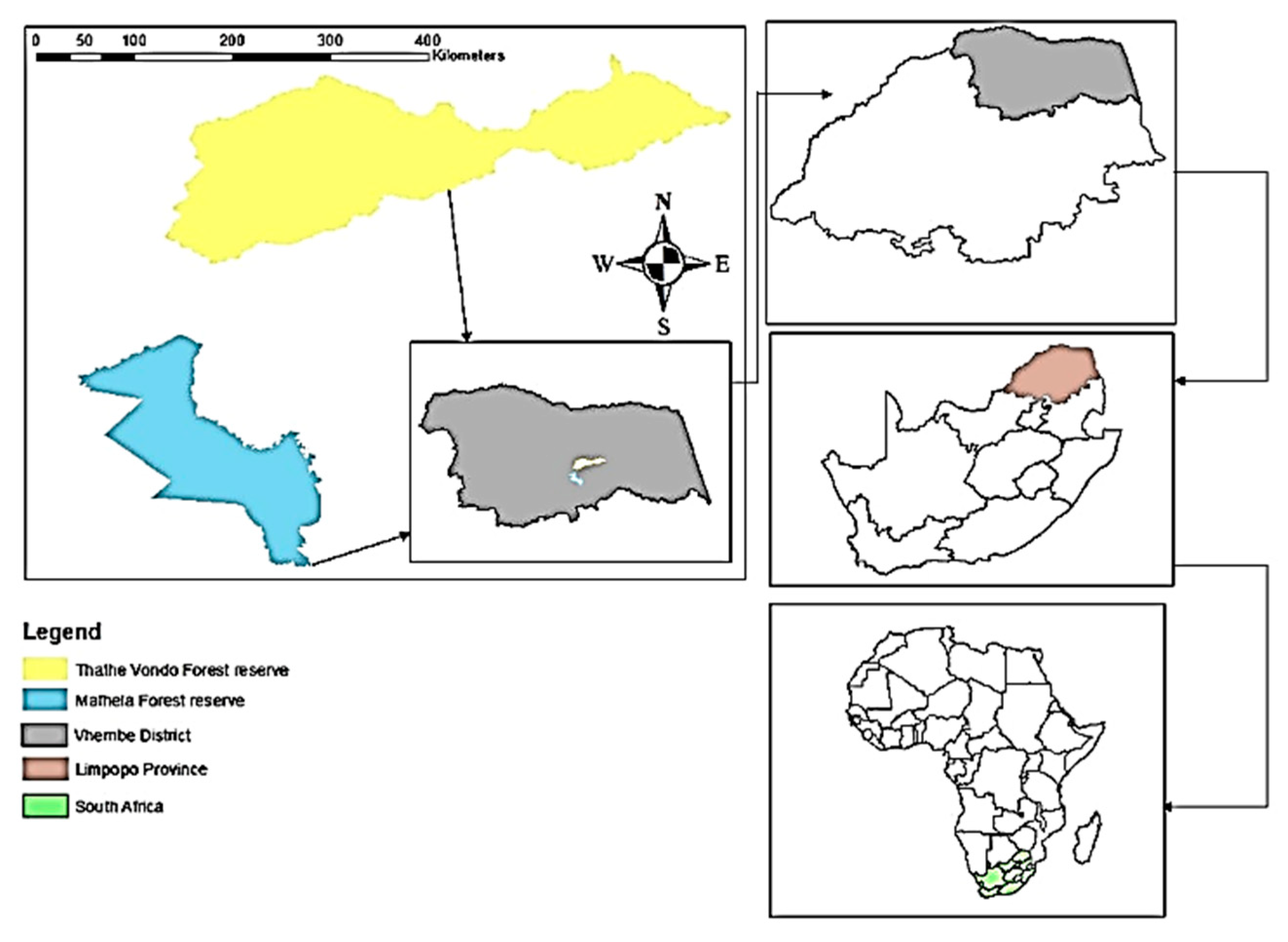
2.1. Study Area

This study was conducted at Mafhela Forest and Thathe Vondo Reserves in the Vhembe Human Biosphere Reserve (VBR) located in Limpopo Province of South Africa. The two Forest Reserve areas (FR) belong to the eastern part of Soutpansberg Mountain Forest complex that stretches from Louis Trichardt to Thohoyandou. Thathe Vondo (TVFR) and Mafhela Forest Reserves (MFR) are located at 22°52′ S, 30°20′ E and 23°01′ S, 30°30.35′ E, respectively (Figure 1). Both Reserves have an altitudinal range of 700–1700 m above sea level. The areas receive rainfall from October to March (on average-724 mm), and the average temperature ranges from 35 °C in summer to 18 °C in winter. Both Forest Reserves retain some of the remaining moist forest cover in South Africa [33]. Notwithstanding, local people residing within the boundaries of the Reserves still practice various tree-based traditional land use, whose potential impact on conservation is unknown.

For this study, the existing land use regimes were classified, in consultation with traditional leaders, based on the configuration of trees, their typical land use, cultural practices, protection gradient, and their management system [34,35]. The existing tree-based traditional land use regimes of the two Forest Reserves were grouped into two major groups as follows:

(a)

Human modified landscape (HMFL): consisting of three tree-based traditional land use regimes under the custody of traditional authorities and the local community. These are:

(b)

Trees Along Streams and Rivers (TATR): local community members are not allowed to harvest live trees, but occasionally access the place for livestock grazing, watering, and shading (intermediately disturbed);

(c)

Common Resource Use Zones (CRUZ): this is an open access area for the harvesting of wild food, construction materials, livestock browsing and grazing, traditional medicines and others (highly disturbed);

(d)

Culturally Protected Forest Areas (CPA): these include sacred/holy forests that are protected by royal families for cultural values and only accessible to them (minimally disturbed).

(e)

State indigenous forests (SIF): these are fragmented forest patches, with minimal to no human disturbance and are legally protected by government conservation agencies.

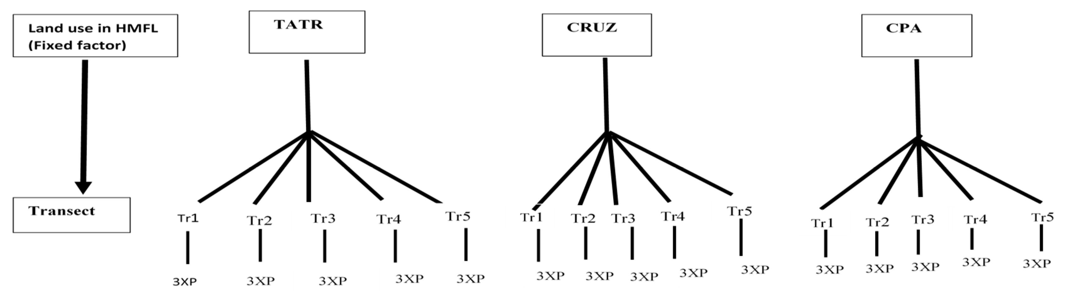
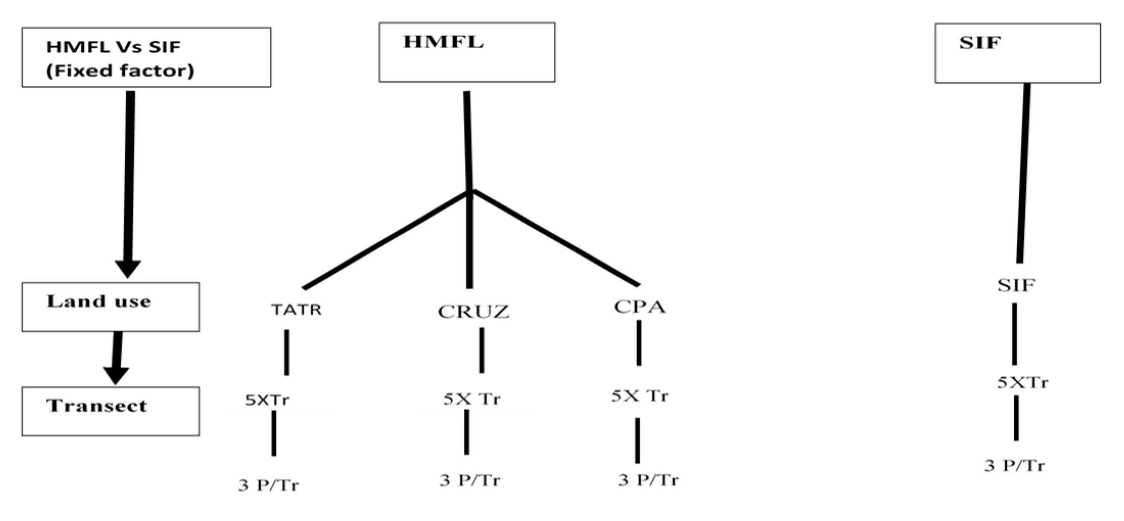
2.2. Sampling Design

Three different asymmetrical nested sampling designs with hierarchical factors relevant to the hypotheses and objectives of the research were adopted after Anderson et al. [36]. To analyze the first hypothesis on β-diversity along the land use gradient in HMFL of the FR and the conformity to IDH, two factors -Transect (Tr) and land use regime (La) were considered. The transect was nested under land use regimes. To determine the effect of land use on β-diversity, land use regimes were kept as a fixed variable (Figure 2).

To compare the overall species richness and the local contribution to β-diversity (LCBD) of HMFLs against SIF (HMFL Vs. SIF) for the second hypothesis, three factors were considered; Transect, land use, and HMFL Vs. SIF. The transects were nested in land use regimes. Land use regimes were nested in HMFL vs. SIF, and HMFL vs. SIF was kept as a fixed factor (Figure 3). Lastly, for the third hypothesis to explore the influence of land use regimes and other environmental change drivers to overall β-diversity of a particular forest Reserve, the plot was nested in Forest Reserves (FR).

Each FR consisted of three land use regimes of the HMFLs (CRUZ, TATR, and CPA) and SIF. Identification and location of land use regimes within the Forest Reserves were done with the guidance of local informants [37,38]. In each land use regime, five transects (Tr) were established. Each transect was 50 m long and separated from each other at least by 200 m. In each transect, three (3) 20 m × 10 m rectangular plots (P) were established and spaced 10 m apart along a linear transect. However, only three transects were used for data collection in TATR in Mafhela Forest Reserve as a large part of the remaining blocks of forest patches had been cleared for horticultural production.

Previous studies in many tropical countries showed that a 40 m × 5 m transect is appropriate for tree species diversity survey [39]. However, in this study, the transect length was 50 m long and each transect was separated from the other ones by at least 200 m. However, unlike other similar studies (e.g., Gillison [40]) that placed four (4) 5 m × 5 m square shaped sample plots in each transect, this study established three (3) 20 m × 10 m rectangular plots (P) that were spaced 10 m apart along a linear transect.

The modification of Gillison [39] and Gillison et al. [40] sampling approaches was important to strike a balance between the observer’s efficiency of data collection and effectiveness of the sampling effort. Experiences in different countries showed that observer fatigue increases if a transect size larger than 40 m × 5 m is used in complex vegetation [41]. Gillison [39] discussed the rough train as a likely factor for observer’s fatigue, which also characterizes the ragged mountain forests of this study area. Hence, the slight increase in transect length combined with the reduction in the number of sample plots per transect was intended to alleviate observer fatigue. At the same time, rectangular sample plots have been proven to capture more species than square shaped sample plots of the same size [41], let alone when using the relatively larger sample plot size covered in this study. The overall sampling area coverage per transect combined with the slight increase in transect length was an attempt to capture a board range of local habitat heterogeneity.

2.3. Data Collection

2.3.1. Measurement of Tree Species Assemblage

In this study, all perennial woody plants with a diameter at breast height (dbh) ≥ 2 cm and height of ≥2 m were considered as trees and enumerated. The scientific and vernacular names (from local informants) of observed tree species in each plot were recorded. In instances where tree species identification was not possible in the field, tree voucher specimens were collected and later identified at the Thohoyandou Botanical Garden and Herbarium.

2.3.2. Change Drivers of Overall β-Diversity of FRs

Land use regime, accessibility, distance from the villages, elevation, slope, and positions of transects within land use and landscape and their geographical locations were recorded. Land use regimes were coded SIF (4), CPA (3), TATR (2), and CRUZ (1) based on a perceived disturbance intensity in ascending order. The elevation of each transect within land use was recorded using GPS. A slope/landscape gradient was recorded using Suunto PM-5/369 PC clinometer. These were grouped and coded as follows: 2°–5° degrees (gentle to undulating—coded 1), 5°–6° degrees (moderate—coded 2), 11°–18° degrees (moderately steep—coded 3), and 19°–30° degrees (steep—coded 4) [42]. The position of each transect was recorded as the bottom, foot-slope, mid-slope, shoulder and top as the landform of the terrain was irregular in both forest areas and coded as 1, 2, 3, 4, and 5, respectively [38]. Distance from the village, which may influence the extent of forest and tree species harvesting by the local community [28], was also estimated in km.

2.4. Statistical Analysis

The effectiveness of the sampling effort on species richness was evaluated using a species accumulation curve based on Bootstrap estimator in Primer-E [43]. An effective sampling effort captures ≥80% of the estimated species richness [44]. This was then followed by comparing the condition of forest landscape complexity of the two Forest Reserves. First, SIMPER (Similarity Percentage) analysis of land use regimes was done on the original abundance matrix to identify dominant species of each FR [36]. SIMPER also provides an output on the contribution of a species to intra-group (within Forest Reserves) similarity by taking the average contribution of ith species (Av. Sim), of overall pairs of sample plots within a group (j, k), of a species in the Bray-Curtis similarity formula (Equation (1)).

$$S_{jk}\left(i\right)=200.\min \left(y_{ik}\right)/{\displaystyle {\sum }_{i=1}^p}\left(y_{ij}+y_{ik}\right)$$

(1)

where S_jk (i) represents the similarity between the Jth and kth sample, y_ij represents the entry in the ith row and J column of the abundance data matrix, that is the abundance for the ith species in the jth sample (i = 1, 2 … p, j = 1, 2 … n).

To describe and compare the spatial patterns of land use disturbance, change drivers for each FRs were subjected to a correlation test using the draftsman plot routine. This is a routine that provides a Spearman correlation coefficient of pairwise variables of all combinations of variables [43].

2.4.1. The Effect of Land Use Regimes on the Difference of Mean β-Diversity in HMFL

To assess the difference in mean β-diversity between land use regimes within each Forest Reserve, first, the information was put into an abundance-based species-sample matrix. The original abundance-based species-sample matrix was transformed into a presence/absence format followed by preparation of the Jaccard similarity coefficient matrix [43]. The Jaccard similarity coefficient calculates the likelihood of a single species being picked at random from two sites without considering the joint absence [36] as follows:

$$S_{jk}\left(i\right)=100\left[\frac{\mathrm{a}}{a+b+c}\right]$$

(2)

where Sjk (i) represents the similarity between the Jth and kth samples and S is the probability (×100). a, b, and c represent the number of species which are present in both samples, the number of species present in sample J but absent from sample in K, and the number of species present in sample K but absent from sample in J, respectively.

First, the Jaccard similarity coefficient matrix was then subjected to non-Metric Multidimensional Scaling Ordination (nNMDS) to visually assess the patterns of mean β-diversity of local assemblage among different land use regimes for HMFLs [43,45]. Points in ordination plot with the same color represent plots within the same land use regime, while the different colors represent different land use regimes. The closeness of points to each other in an ordination plot shows that the degree of similarity of sample points in their local assemblages or lower value for the Jaccard dissimilarity coefficient.

The Jaccard similarity coefficient matrix was subjected to Multivariate analysis of variance in PERMANOVA (permutation-based MANOVA) with 999 permutations to test if there is a statistically significant difference (p ≤ 0.05) in the mean β-diversity of local assemblages (group centroids) among the land use regimes. This was followed by a post-hoc pairwise comparison between land use regimes. To measure the effect size of the difference dissimilarity in mean between pairwise land use regimes, distance from pairwise centroids (Av. D_J) was calculated using a Distance among centroids routine. An Av. D_J takes a percentage value between (0, 100), with the ends of the range representing the extreme possibility; (0) represents identical species assemblages between sample points and (100) represents distinct local assemblages between sample points [36]. Changes in mean β-diversity can happen either due to species richness differences (local extinction/immigration), changes in species composition (replacement of species identity), or both between sample points [46].

2.4.2. Species Richness Difference (Δ $\overline{\mathit{d}}$) along the Land Use Gradient

To determine if there was a significant difference in species richness between land use regimes, the Margalef index (d) for overall species richness was calculated using the DIVERSE function in Primer-E 7 [36]. The Margalef index (d) is an indicator for species richness/count (S) and takes into consideration the effect of size (N) and the fact that within a larger number of individuals, more species are expected [43].

$$d=\frac{\mathrm{S}-1}{\log \mathrm{e}\mathrm{N}}$$

(3)

A resemblances matrix of d-sample plots was then developed using the Euclidean distance. This was analyzed using PERMANOVA (p ≤ 0.05). When PERMANOVA is used to do a univariate ANOVA, the p-values are obtained by permutation, and therefore it avoids the assumption of normality [36]. A pairwise comparison was then used to compare the species richness difference and the conformity to IDH using PERMANOVA. This was done separately for both HMFLs.

Where significant differences were detected, this was then followed by a Hedge (g) metric calculation to detect the effective size of the richness difference between pairs of land use regimes with the same HMFL. The Hedge (g) metric is a weighted average mean standard difference based on a pooled variance measure [45]. It was calculated as follows:

$$g=\frac{X_a-X_b}{SDpooled }$$

(4)

where X_a and X_b refer to the mean of paired samples, and SD_pooled refers to the pooled standard deviation. SD_pooled was calculated as follows:

$$\mathrm{SDpooled}=\sqrt{\frac{\left(n_a-1\right)SD{a}^2+\left(n_b-1\right)SD{b}^2}{n_a+n_b-2}}$$

(5)

where n_a and n_b refers to the sampling size of the paired samples, while SDa² and SDb² refer to the square of the standard deviation of the paired samples.

Since Hedge (g) is a biased estimator of population effective size, we used the commonly used J correction factor to calculate the biased corrected Hedges’ g value or g * = gJ.

$$J=1-\frac{3}{4 \left(n_a+n_b-2\right)-1 }$$

(6)

2.4.3. Change in Species Composition (Identity Replacement) along Land Use Gradient

To determine if there were any significant differences of species composition along the land use gradient, PERMDISP (a test of homogeneity of dispersion) procedure was employed on the Jaccard similarity coefficient matrix (p ≤ 0.05). When PERMDISP is used on the Jaccard similarity coefficient, it provides a test of significance between the sampling points on the identity of species they contain. This was then followed by pairwise comparison on species composition between land use regimes. Also, PERMDISP generates a mean square distance (hereafter referred as mean) of a site to a group centroid (within group dissimilarity) that can directly be interpreted as the percentage of unshared species within a group when the Jaccard dis/similarity matrix is used [36].

2.4.4. A Local Contribution of the Human Modified Forest Landscape to Overall β-Diversity of Forest Reserve

To analyze the impact of human modification of forest landscape on overall structure (variability) of local assemblage, a Jaccard coefficient matrix composed of HMFLs and SIF was organized. The three levels, TATR, CRUZ, and CPA were nested under HMFL (Figure 3). After visually inspecting the patterns of overall mean β-diversity of local assemblage among different HMFLs and SIF using Principal Coordinate Principal Coordinated Analysis (PCA), the Jaccard coefficient matrix was subjected to a PERMANOVA test between HMFLs and SIF for each FR. To analyze the impact of human modification of forest landscape on overall mean species richness (đ_overall), a species richness (d) resemblance matrix of each FR that included SIF was prepared using the same procedures as above. This was then subjected to a PERMANOVA test between HMFLs and SIF for each FR.

To analyze the contribution to HMFLs and SIF to overall β-diversity of the FR, the Jaccard coefficient matrix that was composed of HMFL and SIF was used. Since the PERMANOVA test result showed insignificant difference in mean β-diversity between HMFL and SIF, the Jaccard coefficient matrix was subjected to a pairwise PERMDISP test (test of homogeneity of dispersion) between HMFLs and SIF. When PERMANOVA test result is insignificant for mean β-diversity, PERMDISP result necessarily shows whether the sample plots remained identical or diverge in distinct species assemblage [45]. This was then further inspected using a Principal Coordinate Analysis (PCO) diagram. In the PCO diagram, the site with high LCBD is that found far from the multivariate centroid of the graphs. If a site has large LCBD, it either indicates a high conservation value due to unique assemblage or conversely may indicate a degraded site with poor species assemblage that may need a restoration action [47]. In the context of this study, LCBD was investigated to look at how much, on average, HMFL contributed to unique species assemblage in the FR.

2.5. The Influence of Land Use and Other Environmental Drivers in Overall β-Diversity of Human Modified Forest Reserve

Based on the output of the draftsman plot routine of all change drivers, the multicollinearity test of correlation between all pairs of the change drivers was found to be below the acceptable cut-off threshold (R = 0.95). This was followed by Distance-based linear modeling (DISTLM) and distance-based redundancy analysis (dbRDA) to explore the link between β-diversity with change drivers. DISTLM relies on multiple regression models that can accommodate a mixture of categorical and continuous predictors using dbRDA. This is a constrained ordination of sample sites using the same resemblance matrix on the Jaccard similarity coefficient [36].

The relationship between each environmental variable and overall β-diversity of the FRs was initially analyzed separately (excluding other variables) in the marginal test. Variables were then subjected to a forward selection procedure (sequential test, R² selection criterion), in which the amount of variability explained by each variable added to the model was conditional of the variables already in the model. p-values for the marginal tests were obtained by using 999 permutations and using the Jaccard similarity coefficient matrix. Distance-Based redundancy analysis was used to visualize the results of the DISTLM [36].

3. Result

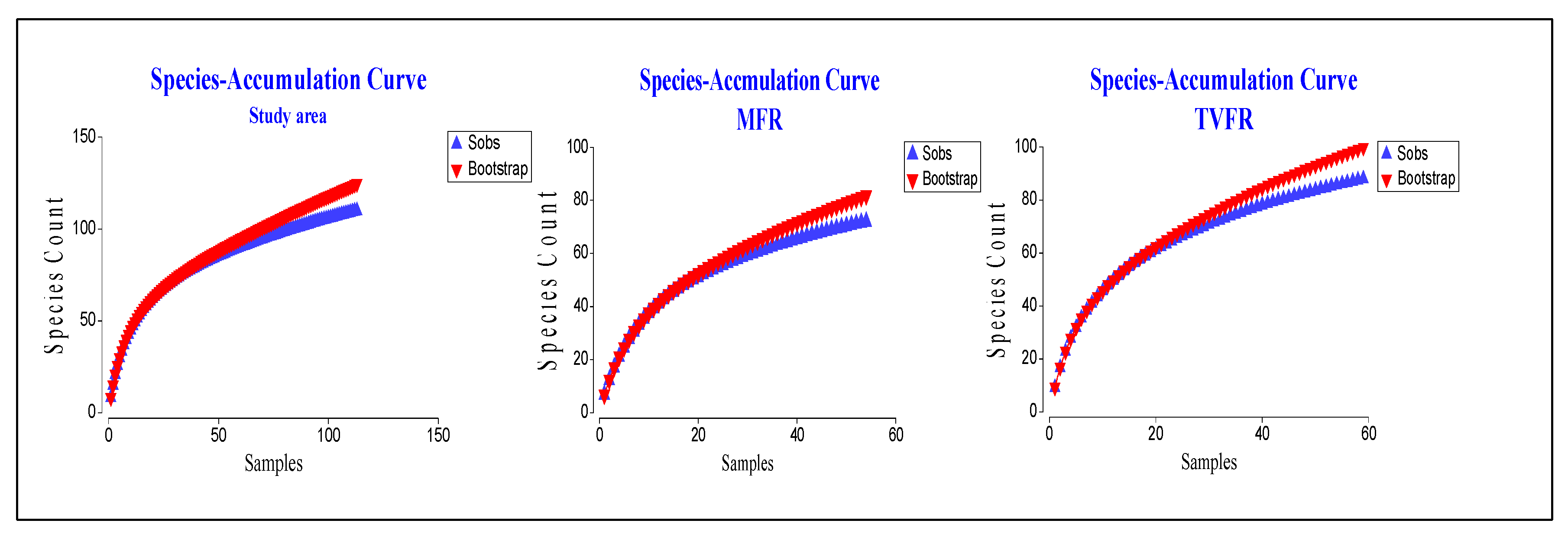
3.1. Description of Forest Complexity Condition

The study recorded 2125 number of individual trees in total; out of which 957 and 1168 number of trees were from MFR and TVFR, respectively. The total number of species observed in the whole study area, in MFR and in TVFR were 110, 72, and 88, respectively. The species accumulation curve based on the Bootstrap technique estimated the whole study area, MFR, and TVFR to host about 125, 82, and 99 species, respectively (Figure 4). Hence, the sampling technique used in this study captured 88.70% of the total species estimated for the whole study, 88.00% for MFR, and 88.18% of TVFR.

In MFR, both the observed and estimated species number showed SIF had relatively the highest number of species, followed by CRUZ, CPA, and TATR in descending order (

Table 1. Observed and estimated species number for land use regimes for MFR (Mafhela Forest Reserve) and TVFR (Thathe Vondo Forest Reserve).

Land Use Regimes	Number of Species in MFR		Sampling Effectiveness (%)	Number of Species in TVFR		Sampling Effectiveness (%)
	Sob	Sboot *		Sob	Sboot *
TATR	18	21	85.71	55	68	80.88
CRUZ	33	39	84.61	57	69	82.61
CPA	26	34	78.80	26	30	86.67
SIF	39	45	86.67	54	65	83.07

TATR = Trees along rivers and streams, CRUZ = Common resource use zone, CPA = Culturally protected forests, S_ob = observed number of species, S_boot * = bootstrap estimated number of species.

). In TVFR, both the observed and estimated species number showed that CRUZ had the highest relative number of species followed by TATR, SIF, and CPA in descending order. Similar to the whole study and Forest Reserves, the sampling technique used in this study also captured the majority of the species in all land use regimes in both Forest Reserves. All the species in the forested landscape were indigenous species to South Africa except Psidium guajava in MFR and Citrus lemon in TVFR in their Common resource use zone.

The SIMPER analysis revealed that the MFR was dominated by seven tree species that contributed about 70% of the total abundance of tree species for the whole landscape, out of which Englerophytum maglismontanum, Bridelia micrantha, and Psidium guajava accounted for about 50% of the total abundance of the trees. In TVFR, 12 tree species dominated and contributed about 70% of the total abundance, out of which Syzygium gerrardii, Xymalos monospora, Englerophytum maglismontanum, Aphloia theiformis, Podocarpus falcatus, and Cassine eucleiformis accounted for 50% of the total abundance of the tree of the landscape.

Table 2. Spearman correlation matrix of land use regimes and other environmental change drivers.

Change Drivers	Thathe Vondo Forest Reserve (TVFR)					Mafhela Forest Reserve (MFR)
	Land Use	Distance	Access	Position	Gradient	Land Use	Distance	Access	Position	Gradient
Distance	−0.58					−0.55
Access	0.24	−0.17				0.24	0.64
Position	0.30	0.48	−0.06			0.17	0.13	−0.08
Gradient	0.19	−0.57	0.24	−0.75		0.04	−0.43	−0.12	0.66
Elevation	−0.31	0.48	−0.47	0.09	−0.14	−0.91	0.74	0.44	−0.06	−0.33

shows that there was a negatively strong correlation between land use intensity gradient and distance from the village in both Forest Reserves. The correlation of land use regime with access, the position of the terrain and slope gradients were weak. However, the two Forest Reserves had substantive differences in strength of correlation coefficient with elevation despite having almost a similar mountain range. While land use intensity gradient had a negative and very strong correlation with elevation in MFR, this correlation was weak in TVFR.

The Effect of Land Use Gradient on of Mean β-Diversity of HMFL

The visual inspection of NMDS in MFR (Figure 5) showed that the local assemblage of all land use regimes in HMFLs was distinct from each other. The PERMANOVA test results in

Table 3. PERMANOVA results for patterns of β-diversity of HMFL along a land use gradient in human modified forest landscape (HMFL) at MFR (Mafhela Forest Reserve) and TVFR (Thathe Vondo Forest Reserve).

HMFLs	Source	Df	SS	MS	Pseudo-F	P(Perm)	Unique Terms
MFR	La	2	44,509	22,254	7.398	0.001	987
	Tr	10	30,082	3008.20	1.537	0.001	996
	Res	26	50,865	1956.30
	Total	38	125,460
TVFR	La	2	31,482	15,741	3.8127	0.001	998
	Tr	12	49,717	4143.10	1.8422	0.001	994
	Res	29	65,222	2249
	Total	43	146,690

Land use gradient (La, fixed factor, three levels) and Transect (Tr, random factor) were nested in La. Degree of Freedom (df), Sum of square (SS), F ratio (Pseudo-F), Permuted probability values (P) are shown.

show that there was a significant dissimilarity in mean β-diversity among different land use regimes in MFR (F₂ = 7.39; p = 0.001). Both pairwise comparison and distance between pairwise centroid (Av. Dj) confirmed that all land use regimes contain highly distinct local assemblage from each other (

Table 4. Pairwise comparison of β-diversity gradient in human modified landscape (HMLF) in Mafhela and ThatheVondo Forest Reserves.

Pairwise Land Use Regimes	HMFLs in MFR			HMFLs in TVFR
	T	p(Perm)	Av. DJ (%)	T	p(Perm)	Av. DJ (%)
(TATR & CRUZ)	2.53	0.016	61	1.59	0.012	38
(TATR & CPA)	2.77	0.022	55	2.22	0.008	51
(CRUZ & CPA)	2.84	0.008	61	2.05	0.006	50

TATR = Trees along rivers and streams, CRUZ = Common resource use zone, CPA = Culturally protected forests, t = pairwise statics value, p = Permuted probability values and Av. D_J = average Jaccard dissimilarity (Percentage).

).

The visual inspection of NMDS in TVFR showed that the local assemblage of all land use regimes is not as distinct as in MFR. Although there was a significant dissimilarity in mean β-diversity among land use regimes in TVFR; (F₁ = 3.81; p = 0.001), the pairwise comparison in TVFR revealed that there was a significant difference among all pairs of land use regimes. However, the distance between pairwise centroid (Av. D_j) showed that (TATR & CRUZ) was fairly similar. Also, the local assemblages between (TATR & CPA) was at the mid-point of the similarity-dissimilarity continuum (Av. D_j = 50%).

3.2. Species Richness along Land Use Intensity Gradient

The overall mean species richness (đ_overall) in Human modified forest landscape in MFR was 2.82 (SD = 0.67). The mean đ (SD) for TATR, CRUZ, and CPA were 2.78 (0.74), 3.19(0.63) and 2.49 (0.46), respectively. PERMANOVA test for species richness (d) showed that there was a significant difference among land use regimes (F₃ = 5.466, p = 0.028) (

Table 5. PERMANOVA results for richness difference between land use intensity in human modified forest landscape (HMFL) at Mafhela (MFR) and Thathe Vondo Forest Reserve (TVFR).

HMFLs	Source	Df	SS	MS	Psuedo-F	P (Perm)	Unique Perms
MFR	La	2	3.740	1.870	5.466	0.029	965
	Tr	10	3.421	0.342	0.970	0.529	999
	Res	26	9.715	0.374
	Total	38	16.876
TVFR	La	2	19.333	9.667	15.454	0.001	998
	Tr	12	7.508	0.626	1.046	0.455	999
	Res	29	17.350	0.598
	Total	43	44.822

Land use gradient (La, fixed factor, three levels) and Transect (Tr, random factor) were nested in La. Degree of Freedom (df), Sum of square (SS), F ratio (Pseudo-F), Permuted probability values (P) are shown.

). However, the pairwise comparison of species richness between (TATR, CRUZ) (t = 1.45, p = 0.26) and between (TATR, CPA) (t = 1.52, p = 0.09) did not detect significant differences.

The overall mean species richness of HMFL in TVFR was 3.78 (SD = 1.02). The đ (SD) for TATR, CRUZ and CPA were 4.62 (0.99), 3.71 (0.69) and 2.96 (0.59), respectively. The PERMANOVA test for species richness difference (Δ $\overline{d}$) found that there was a highly significant difference among land use regimes (F₃ = 15.454, p = 0.001). The pairwise comparison of species richness detected a highly significant difference between (TATR, CRUZ) and between (TATR, CPA) with (t = 3.18, p = 0.03, g = −0.87) and (t = 5.45, p = 0.008, g = −2.57), respectively.

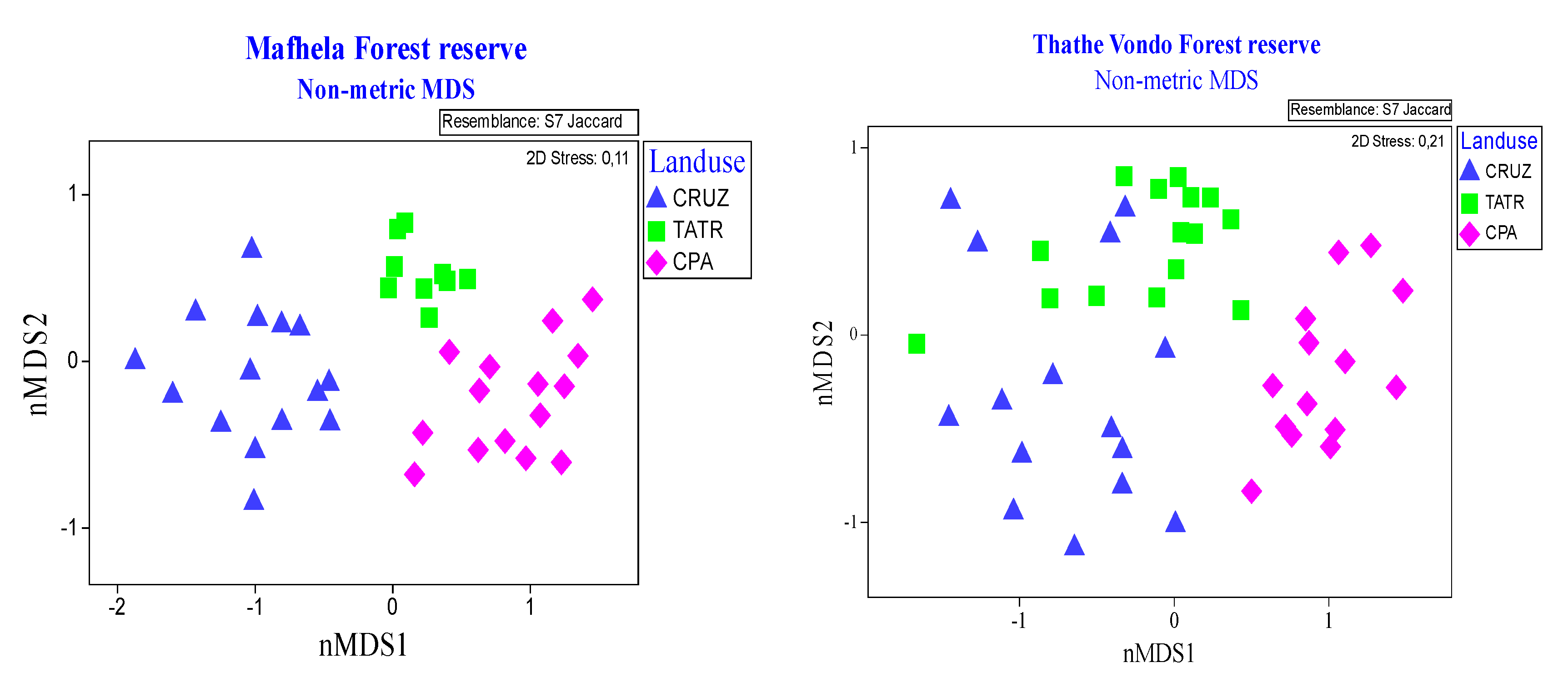
3.3. Change in Species Composition (Identity Replacement) along Land Use Gradients

In MFR, the PERMDISP test showed that there was a significant difference (F_{2, 36} = 9.11, p = 0.001) in species composition along the land use gradient. The pairwise comparison of PERMDISP result showed that there was a significant difference in the species composition between (TATR, CRUZ) and between (TATR, CPA) with (t = 0.002; p = 0.002) and (t = 2.44; p = 0.003), respectively. The local assemblage in TATR, CRUZ, and CPA had about 37.2%, 49.4%, and 44.9% within group dissimilarity (percentage of unshared species), respectively.

In TVFR, PERMDISP test showed a significant difference in species composition among land use regimes (F₂, ₄₁ = 12.69, p = 0.001). However, the pairwise PERMDISP result showed that there was a highly significant difference in species composition between (TATR, CRUZ) (t = 3.03; p = 0.013); but not between (TATR, CPA) (t = 1.42; p = 0.20). The local assemblage in TATR, CRUZ, and CPA had 49.7%, 55.6%, and 46.6% within group dissimilarity, respectively.

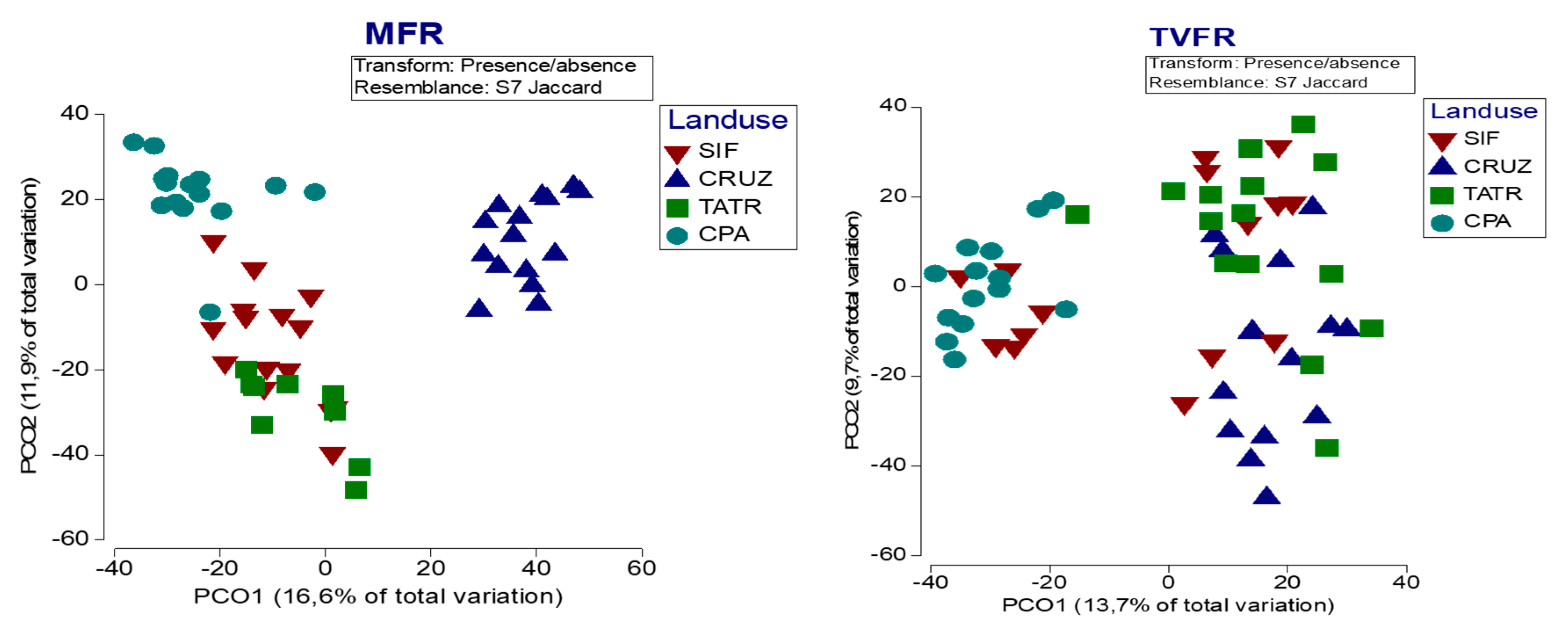
3.4. The Local Contribution of the Human Modified Forest Landscape to Overall β-Diversity of Forest Reserve

The PERMANOVA test result showed that there was no significant difference between the mean β-diversity between (HMFLs, SIF) in both Forest Reserves; (F₁ = 0.68, p = 0.845) in MFR and (F₁ = 0.26, p = 0.817) in TVFR.

The overall mean species richness (đ_overall) of the whole MFR was 3.00, and the standard deviation (SD) was 0.46. The mean đ (SD) for HMFLs and SIF were 2.72 (0.64) and 2.82 (0.67) respectively. PERMANOVA test for species richness difference (Δ $\overline{d}$) between HMFL and SIF confirmed that there was no significant difference (F₁ = 1.98, p = 2.86). The PERMDISP test revealed that there was a significant difference (F_{1, 52} = 16.58, p = 0.001) in within group dissimilarity in species composition between HMLF (Mean = 61.80%) and SIF (Mean = 54.18%). The PCO confirms that most part of the HMFLs contains many sample plots that were further from the ideal local assemblage of the FR than SIF in FR. In particular, PCO 1 showed that CRUZ had a remarkable distinct species assemblage, not with only SIF, but also the other land use regimes with HMFL (Figure 6).

The overall mean species richness (đ_overall) of the whole TVFR was 3.75, and the standard deviation (SD) was 0.93. The mean đ (SD) for HMFLs and SIF part were 3.78 (1.02) and 3.66 (0.61), respectively. PERMANOVA test for species richness difference (Δ $\overline{d}$) between HMFL and SIF found that there was no significant difference (F₁ = 0.014, p = 0.741). The PERMDISP test revealed that there was no significant difference in within group dissimilarity in species composition between HMLF (Mean = 56.6%) and SIF (Mean = 50.5%) (F_{1, 57} = 16.58, p = 0.331). The PCO shows that sample plots in HMFLs and SIF have similar distribution of sample plots from the ideal local assemblage of the FR (Figure 6).

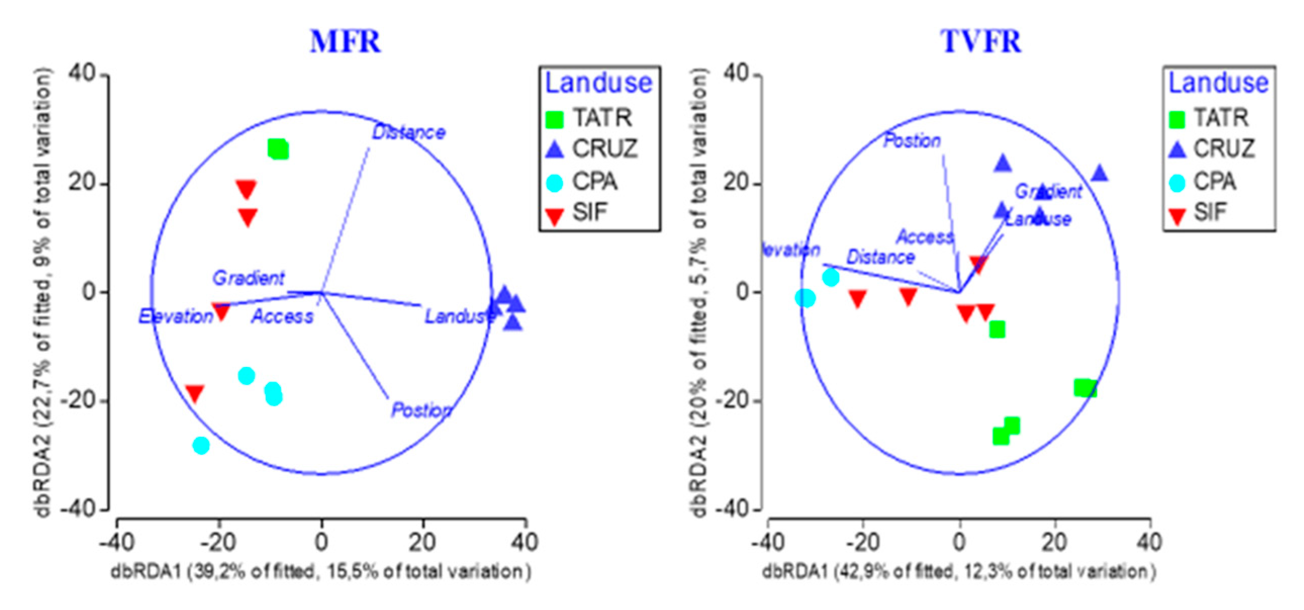
3.5. Change Drivers Influencing Overall β-Diversity of Forest Reserves

The marginal test using DISTLM showed that each element of change drivers was found to be statistically significant in explaining the overall β-diversity of both Forest Reserves. The total sum of the individual contribution of each change driver explains about 53.56% and 38.79% of overall β-diversity in MFR and TVFR, respectively. However, the contribution and the significance of those elements in total explain 39.55% in MFR and 28.63% in TVFR of the overall β-diversity when tested with the sequential test of DISTLM (Figure 7). The drop from the total marginal contribution of each change driver in the sequential test may indicate the prevalence of covariance or interaction of land use and other change drivers in shaping the overall β-diversity patterns of a landscape. In MFR, land use regimes explained the highest portion of (13.85%) of the overall β-diversity pattern. This was then followed by elevation (8.42%), position (9.17%), and distance (8.40%). In TVFR, elevation explained the highest variability (9.8%) followed by a position (5.3%) and slope gradient (3.8%).

4. Discussion

Overall, our sampling technique sufficiently captured the majority of species estimated at all study areas, Forest Reserves, and land use regimes (Figure 2; Table 1). It is evident that anthropogenic disturbance alters the species diversity through a combination of human land use factors by (i) directly removing preferred tree species for livelihood (e.g., fuelwood and timber); (ii) arresting local successional recovery through the recurrent use, including grazing and herbal medicines; (iii) directly or indirectly changing the local conditions (e.g., soil, moisture, sunlight, competition) [48] and; (iv) applying different social norms to govern different parts of a forest landscape [34,35]. Notwithstanding this, the impacts of land use disturbance on biodiversity are neither temporary nor fully avoidable [49]. Furthermore, each landscape, on which different land use intensity is superimposed, is a unique socio-ecological system [26] and differs in their moderating effect on the resilience of local species diversity [30].

The findings from SIMPER and correlational test of land use intensity gradient with other environmental change drivers imply that Mafhela Forest Reserve (MFR) was a relatively simple forest landscape. It had lesser species diversity and dominated by few disturbance tolerant species; on which similar land use regime was spatially clustered across the same elevation range. In contrast, TVFR was complex, species-rich, and dominated by a mix of intermediate and late successional tree species. Unlike MFR, the spatial pattern of land use regimes was more heterogeneous. Hence, a clear understanding of the effect of land use under different conditions of forest landscape complexity in human modified landscapes is crucial for better conservation and management of biodiversity.

Confirming to the hypothesis1, the two HMFLs demonstrated the contrasting effects of land use disturbance to mean β-diversity and conformity to the expectation of IDH. Similar findings of the possibility of divergence and convergence of local assemblages (e.g., reference [21]) and conditional conformity on the response of species richness to intermediate disturbance hypothesis have been reported by many studies (e.g., reference [19]). This can be attributed to the difference in the resilience capacity of the local assemblage of land use regimes due to the variability of landscape moderation to the response of species diversity at different spatial scale [30].

As expected in a simple forest landscape, land use disturbance in MFR enhanced higher dissimilarity in mean β-diversity of local assemblage among all land use regimes. Regardless of the land use intensity gradient, all land use regimes had a distinct local assemblage from each other. This could be because each land use intensity has been creating an environment that suits a set of co-existing species with a similar life-history trait (habitat specialist) [29]. This is consistent with the findings on the lack of conformity of species richness to IDH and the strong evidence of species replacement in HMFLs of MFR. The weak evidence in species richness gradient implies that species replacement played a dominant role in the patterns of β-diversity. Hillebrand et al. [18] underline that when immigration and local extinction (change in species composition) become frequent in a landscape, the species richness can still recover over time to the same level despite the change of species composition.

Furthermore, the higher dissimilarity along a land use gradient in MFR also hints at the limited influence of landscape species pool and the breakdown of ecological connectivity of the landscape (ecological fragmentation) due to the homogenous spatial patterns of land use intensity across the landscape [50]. Ecological fragmentation hinders the recovery of species composition of a vulnerable landscape through natural succession. Conversely, it may enhance further divergence into a set of alternative stable states in the landscape over time [21].

Contrastingly, in a relatively complex forest landscape of TVFR, the local assemblage of land use regimes shared the majority of species among each other. However, the similarity in local assemblage declined along the land use gradient. Such a pattern hints at the higher influence of landscape species pool, ecological connectivity [51], and the positive influence of forest landscape complexity during disturbance-recovery [30]. The conformity of species richness response to IDH in the presence of clear gradient in mean β-diversity hints at the fact that species replacement was practically insignificant to override an orderly local extinction/gain gradient of the TVFR. Hence, the observed β-diversity patterns in HMFLs can be explained by how disturbance affects the mechanisms of species coexistence in a relatively complex landscape.

As expected in the IDH, the intermediately disturbed TATR had a maximum species richness by delaying the competitive exclusion or promotion of co-existence between different life-history traits. The similarity of species shared by CPA and CRUZ with TATR (pairwise D_J), indicates that TATR retained the majority of competitively inferior species of CRUZ as well as the competitively dominant species of CPA that could have become locally extinct under too rare or severe disturbance regimes [7,19]. The severe decline in species richness in local assemblages between (CPA, TATR) may imply that the better traditional protection of CPA resulted in a very severe local extinction of competitively inferior species due to a competitive dominance of a few late successional species.

The findings in TVFR are not surprising considering the recent claim by Munyati and Sinthumule [51] on the decline of deforestation rate and recovery of forest conditions in TVFR vegetation. The conformity of species richness response to IDH may hint that the local assemblage of land use regimes (along a land use intensity gradient) in HMFL in TVFR are more resilient to land use disturbance. However, resilience does not mean the absence of dynamism. Even in the absence of human disturbance, the neighborhood effect, together with biotic and abiotic elements, may still incur small scale changes in species composition [23].

Overall, the higher local contribution of HMFLs to overall β-diversity in MFR through different land use activities might be contributed substantively to γ-diversity (overall biodiversity) of the landscape. The contribution might also appear as a confirmation for the recent criticism on the insufficiency of some protected areas to cover the scale of compositional dissimilarity (e.g., references [2,13]). However, higher overall β-diversity does not automatically imply that human modification of forest landscape enhances the quality and amount of biodiversity [24]. For instance, the highest contribution of CRUZ in MFR to LCBD implies that the substantial proportion of the HMFL was a degraded ecosystem wherein the substantive parts of the original biota were replaced by competitively inferior and early successional species at the local level.

The fact that land use regimes followed by distance and elevation explain the most substantial proportion of overall β-diversity (Section 3.5) highlights that the current condition of forest complexity at a landscape level is highly simplified by anthropogenic disturbance. As such, the landscape species pool may not prevent the local extinction of old-growth tree species [32] unless it is restored. Instead, in line with the intermediate landscape complexity hypothesis [30], the state-protected indigenous forests (SIF) appeared to be more effective in safeguarding species-rich hotspots of a vulnerable landscape. However, when considering the findings of Laurance et al. [30] on the impact of environmental deterioration outside of the majority of tropical protected areas for the ecological health of the interior part of protected areas, even the sustainability of the remaining relatively species-rich SIF is uncertain. This is mainly due to the reduction of the minimum dynamic area required for proper ecosystem functioning [52] and a desperate demand for forest products for rural livelihoods. The shift in local species composition may have a detrimental effect on ecosystem provision to the local community.

In a contrasting ecological manner, human modification in TVFR did not adversely impact the overall landscape assemblage and had equal mean local species richness and LCBD. Following the landscape moderated insurance hypothesis [30], the presence of better conditions of forest landscape complexity might have been assisting in a rapid recovery of ecological process under a continuous land use pressure [32]. The fact that natural factors, such as elevation, slope gradient, and position of the terrain are leading drivers to explain the overall β-diversity shows that human modification did not override the natural gradient of γ-diversity. Instead it kept the species diversity in a dynamic equilibrium. Natural factors become ecologically important when the anthropogenic impact disturbance is minor or when disturbances are widespread and fairly uniformly distributed across a landscape [31]. As such, the effectiveness of SIF in TVFR is lower than its counterpart in MFR. The cumulative impact of land use on HMFL did result in comparable average local species richness and a contribution to overall β-diversity with their counterpart SIF.

5. Conclusions

With the recent prediction of mass extinction of species and the decline of ecosystem services, the debate on whether to maximize on the potential of human modified forest landscapes as an alternative or complementary strategy to protected areas is a non-trivial issue. However, the response for the effectiveness of both conservation alternatives lies in our understanding and response to the question: under what conditions does anthropogenic disturbance enhance, erode, or remain harmless to the pre-existing natural forest conditions in the human biosphere? The contrasting findings between the simple and the complex human modified forest landscape reflect the contrasting insurance value of existing conditions of forest landscape complexity between the HMFLs of the two Forest Reserves. They also reflect that the resilience capacity of local assemblages due to land use pressure can neither be fully explained by one theory nor captured by one species diversity matrix (e.g., Richness or beta-diversity). Using the species richness index alone may obscure the effect of area by averaging the local species richness without discerning the colonization and extinction dynamics. Hence, this situation demands the application of complementary theoretical frameworks and multilevel modeling.

The higher dissimilarity of local assemblages, in the absence of conformity of species richness response to IDH, of a simplified MFR may imply that the replacement of original forest biota in HMFLs is a function of the local extinction of intermediate and late successional species in the whole Forest Reserve. Conversely, a higher species richness of state-protected indigenous forests implies that strictly protected areas can be an effective conservation tool to protect biodiversity hotspots in a simplified forest landscape. They can serve as refugia and source of propagules for the recovery of the local lost species if complemented with restoration efforts for the overall forest landscape complexity. Moreover, reconfiguring the spatial patterns of land use regimes across the HMFLs to increase landscape connectivity may also play a crucial role in restoration. In contrast, maintaining collaborative and holistic landscape management in TVFR, using IDH as a guiding tool, may ensure the sustainability of the current forest landscape complexity and the retention of the rich species diversity. However, conclusive remarks cannot be made based on beta-diversity, since it is only exclusively dependent on presence/absence data. Further research is needed using abundance based data to explictly expose which species traits and their relative abundance would be most affected by any disturbance. This will help to efficiently allocate increasingly limited conservation resources for the conservation of priority species and habitats.

References

1. Harvey, E.; Gounand, I.; Ward, C.L.; Altermatt, F. Bridging ecology and conservation: From ecological networks to ecosystem function. J. Appl. Ecol. 2017, 54, 371–379. [Google Scholar] [CrossRef] [Green Version]
2. Watson, J.E.; Dudley, N.; Segan, D.B.; Hockings, M. The performance and potential of protected areas. Nature 2014, 515, 67. [Google Scholar] [CrossRef] [PubMed]
3. Melo, F.P.; Arroyo-Rodríguez, V.; Fahrig, L.; Martínez-Ramos, M.; Tabarelli, M. In the hope for biodiversity-friendly tropical landscapes. Trends Ecol. Evol. 2013, 28, 462–468. [Google Scholar] [CrossRef] [PubMed]
4. Mittermeier, R.A.; Turner, W.R.; Larsen, F.W.; Brooks, T.M.; Gascon, C. Global biodiversity conservation: The critical role of hotspots. In Biodiversity Hotspots; Springer: Berlin/Heidelberg, Germany, 2011; pp. 3–22. [Google Scholar]
5. Willig, M.R.; Presley, S.J. Biodiversity and disturbance. Encycl. Anthr. 2018, 3, 45–51. [Google Scholar]
6. Van Gemerden, B.S.; Olff, H.; Parren, M.P.; Bongers, F. The pristine rain forest? Remnants of historical human impacts on current tree species composition and diversity. J. Biogeogr. 2003, 30, 1381–1390. [Google Scholar] [CrossRef]
7. Connell, J.H. Tropical rainforests and coral reefs as open non-equilibrium systems. In Population Dynamics; Blackwell: Oxford, UK, 1979; pp. 141–163. [Google Scholar]
8. Fox, J.W. The intermediate disturbance hypothesis should be abandoned. Trends Ecol. Evol. 2013, 28, 86–92. [Google Scholar] [CrossRef] [PubMed]
9. Barlow, J.; Gardner, T.A.; Louzada, J.; Peres, C.A. Measuring the conservation value of tropical primary forests: The effect of occasional species on estimates of biodiversity uniqueness. PLoS ONE 2010, 5, e9609. [Google Scholar] [CrossRef]
10. Noble, I.R.; Dirzo, R. Forests as human-dominated ecosystems. Science 1997, 277, 522–525. [Google Scholar] [CrossRef] [Green Version]
11. Saura, S.; Bertzky, B.; Bastin, L.; Battistella, L.; Mandrici, A.; Dubois, G. Protected area connectivity: Shortfalls in global targets and country-level priorities. Biol. Conserv. 2018, 219, 53–67. [Google Scholar] [CrossRef]
12. Alroy, J. Effects of habitat disturbance on tropical forest biodiversity. Proc. Natl. Acad. Sci. USA 2017, 114, 6056–6061. [Google Scholar] [CrossRef] [Green Version]
13. Joppa, L.N.; Pfaff, A. High and far: Biases in the location of protected areas. PLoS ONE 2009, 4, e8273. [Google Scholar] [CrossRef] [PubMed]
14. Lele, S.; Wilshusen, P.; Brockington, D.; Seidler, R.; Bawa, K. Beyond exclusion: Alternative approaches to biodiversity conservation in the developing tropics. Curr. Opin. Environ. Sustain. 2010, 2, 94–100. [Google Scholar] [CrossRef]
15. Arroyo-Rodríguez, V.; Melo, F.P.; Martínez-Ramos, M.; Bongers, F.; Chazdon, R.L.; Meave, J.A.; Norden, N.; Santos, B.A.; Leal, I.R.; Tabarelli, M. Multiple successional pathways in human-modified tropical landscapes: New insights from forest succession, forest fragmentation and landscape ecology research. Biol. Rev. 2017, 92, 326–340. [Google Scholar] [CrossRef] [PubMed]
16. Resasco, J.; Bruna, E.M.; Haddad, N.M.; Banks-Leite, C.; Margules, C.R. The contribution of theory and experiments to conservation in fragmented landscapes. Ecography 2017, 40, 109–118. [Google Scholar] [CrossRef] [Green Version]
17. Yeboah, D.; Chen, H.Y. Diversity–disturbance relationship in forest landscapes. Landsc. Ecol. 2016, 31, 981–987. [Google Scholar] [CrossRef]
18. Hillebrand, H.; Blasius, B.; Borer, E.T.; Chase, J.M.; Downing, J.A.; Eriksson, B.K.; Filstrup, C.T.; Harpole, W.S.; Hodapp, D.; Larsen, S.; et al. Biodiversity change is uncoupled from species richness trends: Consequences for conservation and monitoring. J. Appl. Ecol. 2018, 55, 169–184. [Google Scholar] [CrossRef] [Green Version]
19. Yuan, Z.Y.; Jiao, F.; Li, Y.H.; Kallenbach, R.L. Anthropogenic disturbances are key to maintaining the biodiversity of grasslands. Sci. Rep. 2016, 6, 22132. [Google Scholar] [CrossRef] [Green Version]
20. Assede, E.S.; Adomou, A.C.; Sinsin, B. Secondary succession and factors determining change in soil condition from fallow to savannah in the Sudanian Zone of Benin. Phytocoenologia 2012, 42, 181–189. [Google Scholar] [CrossRef]
21. Laurance, W.F.; Nascimento, H.E.; Laurance, S.G.; Andrade, A.; Ewers, R.M.; Harms, K.E.; Luizao, R.C.; Ribeiro, J.E. Habitat fragmentation, variable edge effects, and the landscape-divergence hypothesis. PLoS ONE 2007, 2, e1017. [Google Scholar] [CrossRef]
22. Derroire, G.; Balvanera, P.; Castellanos-Castro, C.; Decocq, G.; Kennard, D.K.; Lebrija-Trejos, E.; Leiva, J.A.; Odén, P.C.; Powers, J.S.; Rico-Gray, V.; et al. Resilience of tropical dry forests—A meta-analysis of changes in species diversity and composition during secondary succession. Oikos 2016, 125, 1386–1397. [Google Scholar] [CrossRef] [Green Version]
23. Ghazoul, J.; Burivalova, Z.; Garcia-Ulloa, J.; King, L.A. Conceptualizing forest degradation. Trends Ecol. Evol. 2015, 30, 622–632. [Google Scholar] [CrossRef] [PubMed]
24. Socolar, J.B.; Gilroy, J.J.; Kunin, W.E.; Edwards, D.P. How Should Beta-Diversity Inform Biodiversity Conservation? Trends Ecol. Evol. 2016, 31, 67–80. [Google Scholar] [CrossRef] [PubMed] [Green Version]
25. Legendre, P.; Gauthier, O. Statistical methods for temporal and space–time analysis of community composition data. Proc. R. Soc. B Biol. Sci. 2014, 281, 20132728. [Google Scholar] [CrossRef] [PubMed] [Green Version]
26. Sharma, D.; Holmes, I.; Vergara-Asenjo, G.; Miller, W.N.; Cunampio, M.; Cunampio, R.B.; Cunampio, M.B.; Potvin, C. A comparison of influences on the landscape of two social-ecological systems. Land Use Policy 2016, 57, 499–513. [Google Scholar] [CrossRef] [Green Version]
27. Zhang, J.T.; Xu, B.; Li, M. Vegetation patterns and species diversity along elevation and disturbance gradients in the Baihua Mountain Reserve, Beijing, China. Mt. Res. Dev. 2013, 33, 170–178. [Google Scholar] [CrossRef]
28. Shova, T.; Hubacek, K. Drivers of illegal resource extraction: An analysis of Bardia National Park, Nepal. J. Environ. Manag. 2011, 92, 156–164. [Google Scholar] [CrossRef]
29. Johnstone, J.F.; Allen, C.D.; Franklin, J.F.; Frelich, L.E.; Harvey, B.J.; Higuera, P.E.; Mack, M.C.; Meentemeyer, R.K.; Metz, M.R.; Perry, G.L.; et al. Changing disturbance regimes, ecological memory, and forest resilience. Front. Ecol. Environ. 2016, 14, 369–378. [Google Scholar] [CrossRef]
30. Tscharntke, T.; Tylianakis, J.M.; Rand, T.A.; Didham, R.K.; Fahrig, L.; Batary, P.; Bengtsson, J.; Clough, Y.; Crist, T.O.; Dormann, C.F.; et al. Landscape moderation of biodiversity patterns and processes-eight hypotheses. Biol. Rev. 2013, 87, 661–685. [Google Scholar] [CrossRef]
31. Allan, J.D. Landscapes and riverscapes: The influence of land use on stream ecosystems. Annu. Rev. Ecol. Evol. Syst. 2004, 35, 257–284. [Google Scholar] [CrossRef] [Green Version]
32. Pardini, R.; de Arruda Bueno, A.; Gardner, T.A.; Prado, P.I.; Metzger, J.P. Beyond the fragmentation threshold hypothesis: Regime shifts in biodiversity across fragmented landscapes. PLoS ONE 2010, 5, e13666. [Google Scholar] [CrossRef]
33. Symes, C.T.; Olaf Wirminghaus, J.; Downs, C.T.; Louette, M. Species richness and seasonality of forest avifauna in three South African Afromontane forests. Ostrich 2002, 73, 106–113. [Google Scholar] [CrossRef]
34. Araia, M.G.; Chirwa, P.W. Revealing the Predominance of Culture over the Ecological Abundance of Resources in Shaping Local People’s Forest and Tree Species Use-behavior: The Case of the Vhavenda People, South Africa. Sustainability 2019, 11, 3143. [Google Scholar] [CrossRef] [Green Version]
35. Araia, M.G.; Chirwa, P.W. Nurturing forest resources in the Vhavenda community, South Africa: Factors influencing non-compliance behaviour of local people to state conservation rules. South. For. J. For. Sci. 2019, 81, 357–366. [Google Scholar] [CrossRef]
36. Anderson, M.; Gorley, R.N.; Clarke, R.K. Permanova+ for Primer: Guide to Software and Statistical Methods; PRIMER-E-2015; Primer-E Limited: Plymouth, UK, 2008. [Google Scholar]
37. Sheil, D.; Puri, R.; Wan, M.; Basuki, I.; van Heist, M.; Liswanti, N. Recognizing local people’s priorities for tropical forest biodiversity. AMBIO A J. Hum. Environ. 2006, 35, 17–24. [Google Scholar] [CrossRef] [PubMed] [Green Version]
38. Sheil, D.; Puri, R.K.; Basuki, I.; van Heist, M.; Wan, M.; Liswanti, N.; Sardjono, M.A.; Samsoedin, I.; Sidiyasa, K.; Permana, E.; et al. Exploring Biological Diversity, Environment, and Local People’s Perspectives in Forest Landscapes: Methods for a Multidisciplinary Landscape Assessment; CIFOR SMK Grafika Desa Putera: Jakarta, Indonsia, 2002. [Google Scholar]
39. Gillison, A.N. A Field Manual for Rapid Vegetation Classification and Survey for General Purposes; Centre for International Forestry Research: Bogor, Indonsia, 2006. [Google Scholar]
40. Gillison, A.N.; Liswanti, N.; Rachman, I.A. Rapid Ecological Assessment of Kerinci Seblat National Park Buffer Zone; Centre for International Forestry Research: Bogor, Indonsia, 1996. [Google Scholar]
41. Hairiah, K.; Sitompul, S.M.; van Noordwijk, M.; Palm, C. Methods for Sampling Carbon Stocks above and below Ground; ICRAF: Nairobi, Kenya, 2001; pp. 1–23. [Google Scholar]
42. Young, A. Tropical Soils and Soil Survey; Cambridge University Press: Cambridge, UK, 1980; Volume 9. [Google Scholar]
43. Clarke, K.R.; Gorley, R.N.; Anderson, M.A. Change in Marine Communities: An Approach to Statistical Analysis and Interpretation, 3rd ed.; PRIMER-E-2015; Primer-E Limited: Plymouth, UK, 2015. [Google Scholar]
44. Foggo, A.; Attrill, M.J.; Frost, M.T.; Rowden, A.A. Estimating marine species richness: An evaluation of six extrapolative techniques. Mar. Ecol. Prog. Ser. 2003, 248, 15–26. [Google Scholar] [CrossRef] [Green Version]
45. Avolio, M.L.; Pierre, K.J.L.; Houseman, G.R.; Koerner, S.E.; Grman, E.; Isbell, F.; Johnson, D.S.; Wilcox, K.R. A framework for quantifying the magnitude and variability of community responses to global change drivers. Ecosphere 2015, 6, 1–14. [Google Scholar] [CrossRef]
46. Coetzee, B.W.; Gaston, K.J.; Chown, S.L. Local scale comparisons of biodiversity as a test for global protected area ecological performance: A meta-analysis. PLoS ONE 2014, 9, e105824. [Google Scholar] [CrossRef]
47. Legendre, P. Interpreting the replacement and richness difference components of beta diversity. Glob. Ecol. Biogeogr. 2014, 23, 1324–1334. [Google Scholar] [CrossRef]
48. Mayor, S.J.; Cahill, J.F., Jr.; He, F.; Boutin, S. Scaling disturbance instead of richness to better understand anthropogenic impacts on biodiversity. PLoS ONE 2015, 10, e0125579. [Google Scholar] [CrossRef] [Green Version]
49. Ellis, E.C.; Antill, E.C.; Kreft, H. All is not loss: Plant biodiversity in the Anthropocene. PLoS ONE 2012, 7, e30535. [Google Scholar] [CrossRef] [Green Version]
50. Li, S.P.; Cadotte, M.W.; Meiners, S.J.; Pu, Z.; Fukami, T.; Jiang, L. Convergence and divergence in a long-term old-field succession: The importance of spatial scale and species abundance. Ecol. Lett. 2016, 19, 1101–1109. [Google Scholar] [CrossRef] [PubMed]
51. Munyati, C.; Sinthumule, N.I. Cover Gradients and the Forest-Community Frontier: Indigenous Forests under Communal Management at Vondo and Xanthia, South Africa. J. Sustain. For. 2014, 33, 757–775. [Google Scholar] [CrossRef]
52. Hansen, A.J.; DeFries, R. Ecological mechanisms linking protected areas to surrounding lands. Ecol. Appl. 2007, 17, 974–988. [Google Scholar] [CrossRef] [PubMed]
Figure 1. Location of the study area in the Vhembe Biosphere Reserve in Limpopo Province, South Africa.
Land 09 00004 g001
Figure 2. Schematic diagram of the sampling design of β-diversity in Human Modified Forest Landscape (HMFL) of the Forest Reserves (FR) and the conformity to Intermediate Disturbance Hypothesis (IDH). TATR = Trees Along Rivers and Streams, CRUZ = Common Resource Use Zone, CPA = Culturally Protected Forests, Tr = Transect.
Land 09 00004 g002
Figure 3. Schematic diagram of the sampling design to compare the overall species richness and the local contribution to β-diversity of Human Modified Forest Landscape (HMFLs) against SIF (HMFL vs. SIF) for the second hypothesis.
Land 09 00004 g003
Figure 4. Species accumulation curve based on Bootstrap estimators. MFR = Mafhela Forest Reserve, TVFR = Thathe Vondo Forest Reserve.
Land 09 00004 g004
Figure 5. Multi-dimensional scaling (MDS) of local assemblage of different land use regimes in MFR and TVFRs.
Land 09 00004 g005
Figure 6. Principal Coordinate analysis (PCO) of local assemblages among different land use regimes within HMFLs and SIF.
Land 09 00004 g006
Figure 7. dbRDA (Distance-based redundancy analysis) graphs on the relationship of land use regimes (based on land use intensity gradient) and other change drivers to overall β-diversity. MFR = Mafhela Forest Reserve, TVFR = Thathe Vondo Forest Reserve; TATR = Trees along rivers and streams, CRUZ = Common resource use zone, CPA = Culturally protected forests, SIF = State-protected indigenous forest.
Land 09 00004 g007