The Moderate Operation Scales of Apples Based on Output, Profit, and Unit Production Costs in the Shaanxi Province of China

Abstract

In the Shaanxi province, small and scattered plots impede an increase in the efficiency of apple production. Developing a moderate operation scale is a proper tool to solve inefficiencies in apple production, as it enables improving the factor allocation efficiency, resulting in higher yields, higher profit, or lower production costs. However, the moderate operation scales, based on output, profit, and production costs, may be different. This paper aimed to evaluate the moderate operation scale of apples from three perspectives of increasing yields and profits and reducing unit production cost. The study was based on survey data collected from 661 randomly selected apple farmers in eight counties of the Shaanxi province, China. The collected data were analyzed quantitatively by the input-output model, the net profit model, and unit production cost model. The findings show that: (1) The moderate operation scale oriented to increasing apple yields in the Shaanxi province should be 0.87–1.53 ha. (2) The moderate operation scale oriented to increasing the net profit of farmers in the Shaanxi province should be over 1.53 ha. (3) The moderate operation scale oriented to reducing the unit cost of apple production in the Shaanxi province should be 0.20–0.53 ha. The study provides evidence that policymakers should grasp the balance point and find the intersection of the operation scale based on output, profit, and unit production cost when guiding apple growers to carry out the moderate scale. We propose that 0.87–1.53 ha may be a suitable operation scale for apple production in the Shaanxi province at the current stage.

1. Introduction

Starting in the late 1970s, China introduced a land system reform, distributing the rural land proportionally according to the number of persons in the family and transferring the land management right to the farmers. Then, the household contract responsibility system1 was implemented to guide agricultural production, heightening the enthusiasm of farmers for production [1]. This has made positive contributions to boosting agricultural production, increasing farmers’ income and narrowing the income gap between urban and rural areas [2]. However, it also leads to the characteristics of small-scale and fragmented agricultural production in China. Against the background of marketization reform, population transfer, and urban-rural integration, the small-scale operation mode has been increasingly challenged [3]. Innovating the agricultural operation system and expanding the operation scales had been the inevitable choices for agricultural development in China [4,5]. However, the operation scale is not simply a case of the bigger, the better, and we need to find a moderate point. So, deciding on the moderate scale is the key to the development of modern agriculture.

In 1987, the Central Committee of the Communist Party of China first proposed to adopt various forms of moderate operation scales [6]. In 2008, the Decision of the Central Committee of the Communist Party of China clearly called for continuing to develop the moderate operation scale in agriculture in several important documents and decisions. It can be seen that developing the moderate operation scale, rationally allocating the factors of agricultural production, and solving the plight of agricultural development have become important issues that commonly concern policymakers [3]. The connotation of moderate operation scale of agriculture determines its evaluation standards. So, defining “moderate operation scale” was the key. Zhang et al. state that, the “moderate operation scale” refers to the farm size when a household can make full utilization of the labor force and other factors to obtain the best economic benefits under a certain level of productivity and operating environment [7]. According to Ma and Ma, the “moderate operation scale” refers to the farm size whereby a household can achieve the optimal allocation of various production factors to improve the land productivity, reduce the average production cost, and maximize the income through the realization of scale economy [8]. In summary, the moderate operation scale may be an optimal scale interval under certain conditions [9,10].

The existing studies on “moderate operation scale” show the differences between different geographical regions and different historical stages. Generally speaking, four evaluation standards were mainly used to evaluate the moderate scale. The first evaluation standard was land productivity. In the 1990s, abundant studies on the relationship between operation scale and land productivity were carried out, but the conclusions were not consistent. Some studies prove the negative association between land productivity and operation scale [11,12,13,14,15,16,17,18]. For instance, Xu et al.’s study found that increasing farmers’ operation scale did not necessarily lead to more grain production [18]. Some studies prove the positive association between land productivity and operation scale [19,20,21]. For instance, the study of Fan and Zhou found that there was a positive association between land productivity and operation scale [21]. In addition, some studies prove the nonlinear association between operation scale and land productivity. For instance, using panel data of rural household surveys, Ni and Cai found that there was a negative association between land productivity and operation scale among farm households with an operation scale less than 41.07 ha while there was a positive association among others with operation scales greater than 41.07 ha [22]. And they proposed that it was difficult to achieve the operation scale over 41.07 ha for farmers, considering the number of Chinese farmers and land. However, using the household-level data from Jilin province of China, Xin et al.’s study found that land productivity changed in “inverted U-shaped” with the operation scale, and the moderate operation scale should be 2 ha [23].

The second evaluation standard was labor productivity. Using panel data of rural household survey in China, study of Ni and Cai found that labor productivity changed in “inverted U-shape” with the operation scale, and the moderate operation scale of family farms should be 8.73–9 ha while that of large-scale grain-production household should be 15.6–15.73 ha [22]. Using panel data of 31 provinces in China from 2000 to 2013, Wang et al. found that labor productivity changed in “inverted L-shape” with the operation scale, and the moderate operation scale should be 6.25 ha per farmer [24]. They also found that the moderate operation scale in the plain area should be 6.37 ha per farmer while that in hilly area should be 1.98 ha per farmer.

The third evaluation standard was unit production cost. Many studies prove the negative association between unit production costs and operation scale [18,23,25,26]. For instance, Xu et al. found that expanding the operation scale contributed to reducing unit production costs [18]. Song et al. found that, based on unit production cost minimization, the moderate operation scale of rice, soybean and maize should be 1–2 ha, 2–4 ha, and 4–7.67 ha, respectively [26]. Some studies came to the opposite conclusion [27,28,29]. For instance, Li et al. found that there was a positive association between unit production costs and operation scale [28]. In addition, using the household-level data from Jiangsu province of China, Zhang’s study found that unit production costs changed in “U-shape” with the operation scale, and the moderate operation scale should be less than 13.33 ha [29].

The fourth evaluation standard was the net profit of agricultural production. Using the household-level data from Jiangsu and Zhejiang provinces of China, Zhang and Wu’s study found that the net profit per ha changed in “U-shape” with the operation scale, and the moderate operation should be 1.33–1.67 ha [30]. Using rice farmers’ data from 22 provinces of China, Li et al. found that the moderate operation scale of rice should be over 5.33 ha based on net profit maximization [28]. However, using the household-level data from Heilongjiang province of China, Song et al. found that the moderate operation scale of rice should be 1–2 ha based on net profit maximization [26]. In addition, they also found that the moderate operation scale of maize should be 4–7.67 ha based on net profit maximization while there was no limit to the operation scale of soybean.

As mentioned before, whether the operation scale of agricultural production is moderate or not, there are obvious differences in the conclusions based on different evaluation standard and research methods [31,32]. Therefore, some scholars proposed comprehensive standards to evaluate the moderate operation scale of agricultural production [33,34]. For example, Li et al. [28] and Wang et al. [27] evaluated a moderate operation scale of rice based on scale benefit, output level, and production cost. Song et al. [26] evaluated the moderate scale of corn, rice, and soybeans based on the food security and increasing farmers’ income. Xu et al. [18] evaluated the moderate operation scale of spring and winter wheat, early, middle, and late indica rice, japonica rice, and maize in China from the perspectives of input, output, and production cost.

To sum up, the existing literature was mainly focused on the moderate scale of grain crops, while insufficient attention has been paid to high-value agricultural products, in particular, apples. Against the background of people’ income growth and the upgrading of dietary structure in China, the consumption of apples is increasing rapidly. In China, apple production faces three challenges: the first is to increase production to meet people’s growing consumer demand; the second is to increase farmers’ income, and the third is to reduce production costs to improve the competitiveness of the international market. According to the statistical data, the area of apple crops in the Shaanxi province in 2015 reached 628,550 ha, which is the highest in China. How to develop the moderate operation scale of apple farming in Shaanxi Province should be the focus for research. If the operation scale is too small, it cannot achieve the task of ensuring output, promoting income, and reducing cost. If the operation scale is too large, it may reduce the regional agricultural diversity and cause a regional food production crisis. Therefore, this study aims to evaluate the moderate scale of apple production in the Shaanxi province based on output, net profit, and unit production cost. The study uses data from the structured interviews with 661 apple growers from eight counties in Shaanxi Province, China. The purpose is to determine an optimum scale of apple production.

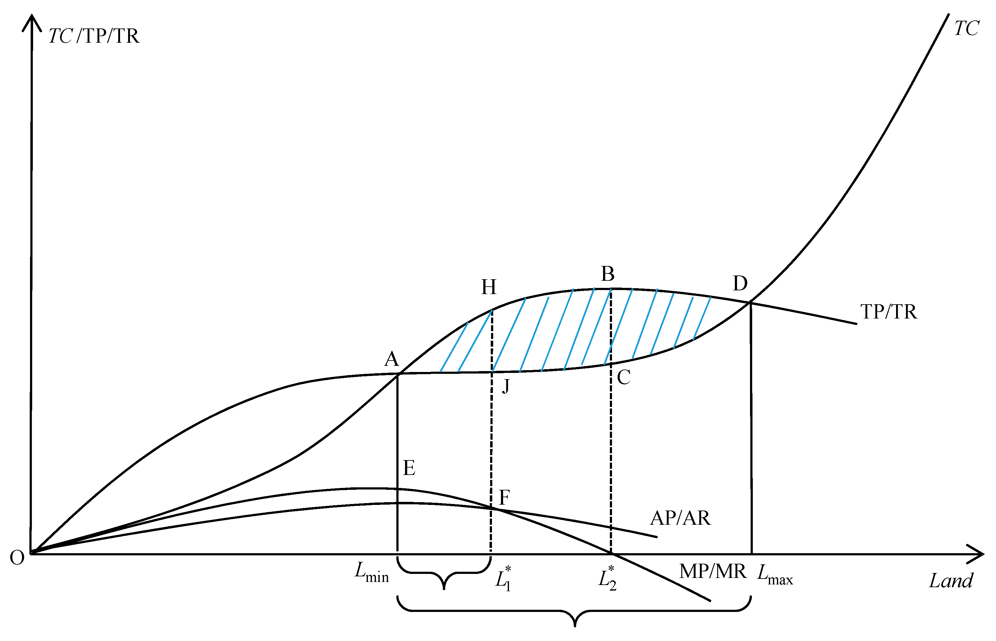
2. The Moderate Operation Scale in Theory

It is assumed that there are three main input factors in apple production, namely labor, capital, and land. According to the theory of diminishing marginal return, if the labor and capital input factors remain unchanged, the change of output caused by the increase of land can be divided into three stages (Figure 1, total production (TP) curve): (1) with marginal production (MP) increasing, the total production increases; (2) with marginal production decreasing, the total production increases; (3) with marginal production less than 0, the total production decreases. In the first stage, the marginal production (MP) increases and reaches the highest point at point E, and MP > AP (Average Production), the average production increases. In the second stage, the marginal production MP decreases, and MP > AP, so the average production continues to increase. When MP = AP (at point F), the average production reaches the maximum, that is, the land productivity reaches the maximum, and the corresponding planting area is L₁*. Therefore, the moderate operation scale oriented to increase apple yields should be (0, L₁*).

According to the theory of diminishing marginal cost, the change of expected total cost of production of farmers can be divided into two stages (Figure 1, total cost (TC) curve): (1) with the marginal cost (MC) decreasing, the total cost increases; (2) with the increase of marginal cost, the total cost increases. Assuming the market price of apples is 1, the total output curve of apple production coincides with the total revenue (TR) curve. The net revenue (△R) of apple production is △R = TR-TC. Assuming that farmers are rational, they will make decision on the operation scale under △R > 0 (the shaded part in Figure 1). The effective scale interval of farmers is [L_min, L_max], which verifies the theoretical viewpoint that there exist minimum and maximum values of the moderate operation scale [9].

As shown in Figure 1, at [L_min, L_max], with the expansion of the operation scale, the marginal revenue (MR) of apple production declines, while the marginal cost decreases first and then rises. When MR = MC = 0 (at point B), the total revenue of apple farmers is the largest, the unit cost of apple production is the lowest, and the net revenue of apple production is the largest. At this time, the corresponding planting area is L₂*. It can be seen that the optimal area for increasing net profit of apple farmers and reducing production costs should be L₂*, then the moderate operation scale oriented to increasing farmers’ net profit is [L_min, L₂*], while the moderate operation scale oriented to reducing unit production cost is (0, L₂*].

3. Study Area and Methods

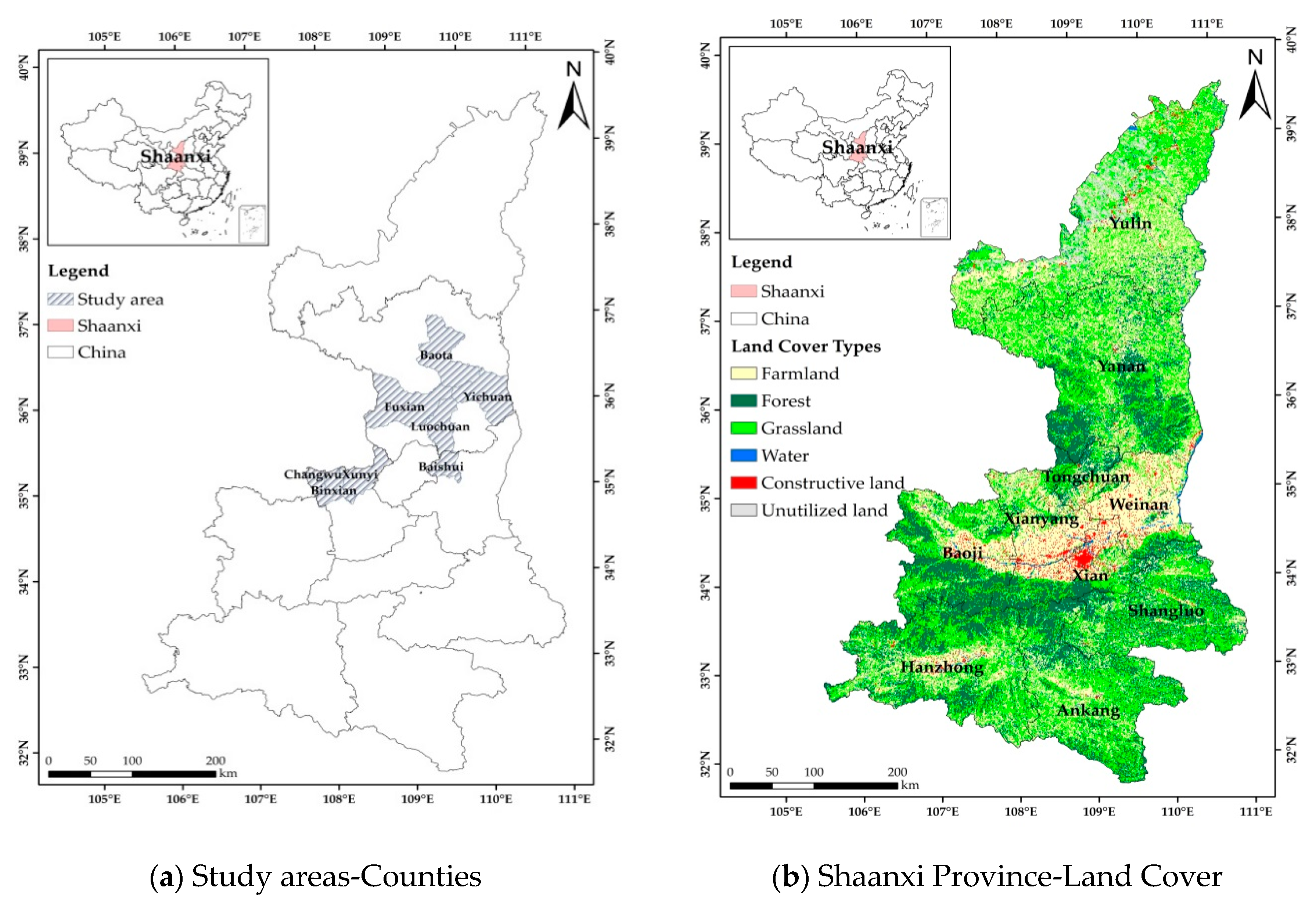
3.1. Description of Study Area

For the purpose of this study, the Shaanxi Province was selected (Figure 1). The Shaanxi Province was purposively selected for this study due to:

• Shaanxi is one of the most important apple planting regions in China, where the area and the quantity of apple production are the biggest.
• The diversity of agro-climatic in Shaanxi is the epitome of the distribution of agroclimatic zone in China.
• The continious expanding of apple planting area in Shaanxi province leading to a more obvious contradiction on how to develop moderate operation scale (The apple planting area was 601,518 ha in 2010 and increased to 695,159 ha in 2015).
• The author’s local knowledge.

The Shaanxi province has a total area of 205,800 km² and nearly 40% is in the region of Loess plateau. Its elevation ranges from 350 to 3500 m above sea level. Due to specific physiographic features and climate conditions, Shaanxi has been one of the most suitable regions for apple production in the world, and it contains 30 base counties for apple production in total. The area of apple production in Shaanxi in 2015 reached 628,550 ha, accounting for 27% of the area in China and 12.3% of the area in the world (Food and Agriculture Organization of the United Nations http://www.fao.org/statistics/en/).

The Shaanxi province has 379,300,00 inhabitants, and the population density is 184 people per km². According to the survey data, the average farm size per household is 0.76 ha in Shaanxi Province.

3.2. Sampling Design, Data Collection, and Statistical Description

In this paper, we use multi-stage sampling techniques to collect the samples. In the first stage, based on the intensity of apple production, eight counties were selected: Changwu, Binxian, Xunyi, Baota, Yichuan, Fuxian, Luochuan, and Baishui (Figure 2). In the second stage, five villages in each selected county were randomly selected. In the third stage, 15–20 households in each village were randomly selected, and 663 households were randomly sampled for interviews in total (81 from Changwu, 82 from Binxian, 83 from Xunyi, 79 from Baota, 85 from Yichuan, 87 from Fuxian, 82 from Luochuan, and 84 from Baishui).

Field data were collected from July 2015 to August 2015. The primary data were collected by household surveys (HHS) with a structured questionnaire. On the basis of the results obtained from the pre-test, necessary modifications were made to the questionnaire. The final questionnaire contains three sections: the demographic and economic characteristics of farmers, the input of factors including labor, land, and capital, and the output and income of apple production. Face to face interviews were necessary, as many of the respondents were expected to be illiterate. Due to lack of major information, two samples were excluded, and the final sample size was 661 completed questionnaires.

Table 1. Statistical description of the sample characteristics.

Major Variables	Mean	SD	Minimum	Maximum
Output of apple production (kg per household)	11,745.46	17,552.97	100.00	70,000.00
Net profit of apple production (¥ per household)	37,154.84	50,732.12	−70,360.00	665,786.00
Total cost of apple production (¥ per household)	27,532.70	20,485.40	1,230.00	191,360.00
Labor input (working days per household)	226.74	244.19	26.50	5,442.00
Capital input (¥ per household)	27,532.74	20,500.95	1,230.00	191,360.00
Operating scale (ha per household)	0.48	4.77	0.03	2.33
Land fragmentation (plots per household)	2.75	1.63	1	16
Gender of household head (dummy)	0.98	0.13	0	1
Age of household head (year)	50.86	8.80	24	75
Educational level of household head (year)	7.92	3.04	0	15
Number of family labors (people per household)	2.13	0.68	1	7

is a statistical description of the sample characteristics. Overall, the average output of the samples is 11,746 kg per household, the average net profit2 was 37,155 ¥ per household, and the average total cost was 27,533 ¥ per household. The average labor input (including family labor and hired labor) was 227 working days per household, the average capital input (including fertilizer, pesticide, and fruit bag costs, depreciation of fixed assets, and mechanical services costs) was 27,533 ¥ per household, and the average operation scale of apples was 0.48 ha per household. Land fragmentation was relatively serious in Shaanxi, and the average number of plots is 2.8 per household. From the demographic and economic characteristics of farmers, 98% of the household heads were men, and the average age of the household head was 51 years old. The average educational years of the household head were 7.9, which is equal to junior middle school level in China.

3.3. Methods of Data Analsis

3.3.1. Model

(1) The moderate operation scale, land fragmentation and output: input–output model.

Currently, the commonly used production functions include the C-D function and the Translog function. Compared with the C-D function, the Translog production function does not impose any restrictions on economies of scale and elasticity of factor substitution, and for any production technology, this function can be better approximated [18]. Therefore, based on the Translog production function, we established an input–output model for farmers to analyze the relationship between operation scale and output level, and compared the differences of output level in different scales of apple production. The model is built as follows:

$$\begin{array}{l}\ln Q_i={\alpha }_0+{\displaystyle \sum _{j=1}^3{\alpha }_j\ln x_{ij}}+\frac{1}{2}{\displaystyle \sum _{j=1}^3{\displaystyle \sum _{j=1}^3{\gamma }_{jj}\ln x_{ij}\ln x_{ij}}}+{\displaystyle \sum _{n=1}^4{\eta }_{n}scale\_dumm{y}_{ni}}+{\delta }_{1}ag{e}_i\\ +{\delta }_{2}ag{e}_i^2+{\delta }_{3}ed{u}_i+{\delta }_{4}l{t}_i+{\delta }_{5}p{y}_i+{\displaystyle \sum _m^2{\lambda }_{m}region\_dumm{y}_{mi}}+{\mu }_i\end{array}$$

(1)

In Equation (1), $Q_i$ denotes the output of apple production, $x_{1i}$ denotes the operation scale of apple, $x_{2i}$ denotes the effective labor input of apple production, including family labor and hired labor, $x_{3i}$ denotes the capital input of apple production, including fertilizer, pesticide, and fruit bag costs, depreciation of fixed assets, and mechanical services costs, and $scale\_dumm{y}_{ni}$ denotes a group of dummy variable reflecting different scales. According to the characteristics of apple production in Shaanxi province and the research conclusions of Qu [35], we divide the operation scale of apple farmers into five sections, including 0–0.20 ha, 0.20–0.53 ha, 0.53–0.87 ha, 0.87–1.53 ha and over 1.53 ha. In this paper, we take 0–0.20 ha as the reference group to set the dummy variable. In addition, based on the findings of previous and current studies on agricultural output [18,26,27,28,36,37], seven explanatory variables were identified. Namely, $ag{e}_i$ denotes the age of the household head, $ag{e}_i^2$ denotes the square term of $ag{e}_i$, $ed{u}_i$ denotes the education years of the household head, $p{y}_i$ denotes production experience and skills of the household head, measured by years of planting, $l{t}_i$ denotes whether land transfer or not, and $region\_dumm{y}_{mi}$ denotes a dummy variable, which is used to reflect the regional differences of apple production. In this paper, we take the farmers in Weinan city as the reference group to set the dummy variable.

Land fragmentation is defined as a situation where farmers are cultivating two or more geographically separated plots of land by taking into account the distances between those parcels [38]. Relevant research shows that land fragmentation may indirectly affect the whole agricultural production process by affecting the use efficiency of input factors [39]. Therefore, in this paper, land fragmentation is introduced into the model in the form of efficiency function ${\varphi }_0$. Referring to the research methods of Xu et al. [18], in this paper, we take the number of plots as the proxy variable of land fragmentation, then can obtain ${\varphi }_0$:

$$\begin{array}{c}{\varphi }_0={\alpha }_0+{\beta }_0\ln Plo{t}_i\\ \mathrm{or}\\ {\varphi }_0={\alpha }_0+{\beta }_{0}Plo{t}_i\end{array}$$

(2)

Assuming that land fragmentation has a neutral impact on apple production, substituting Equation (2) into (1), we obtain the input–output model while considering land fragmentation:

$$\begin{array}{l}\ln Q_i={\alpha }_0+{\beta }_0(plo{t}_i)\ln plo{t}_i+{\displaystyle \sum _{j=1}^3{\alpha }_j\ln x_{ij}}+\frac{1}{2}{\displaystyle \sum _{j=1}^3{\displaystyle \sum _{j=1}^3{\gamma }_{jj}\ln x_{ij}\ln x_{ij}}}+{\displaystyle \sum _{n=1}^4{\eta }_{n}scale\_dumm{y}_{ni}}\\ +{\delta }_{1}ag{e}_i+{\delta }_{2}ag{e}_i^2+{\delta }_{3}ed{u}_i+{\delta }_{4}l{t}_i+{\delta }_{5}p{y}_i+{\displaystyle \sum _m^2{\lambda }_{m}region\_dumm{y}_{mi}}+{\mu }_i\end{array}$$

(3)

Assuming that land fragmentation has a non-neutral impact on apple production, substituting Equation (2) into (1), we obtain the input–output model while considering land fragmentation:

$$\begin{array}{l}\ln Q_i={\alpha }_0+{\beta }_0(plo{t}_i)\ln plo{t}_i+{\displaystyle \sum _{j=1}^3({\alpha }_j+{\beta }_j(plo{t}_i)\ln plo{t}_i)\ln x_{ij}}+{\displaystyle \sum _{j=1}^3{\alpha }_j\ln x_{ij}}+\frac{1}{2}{\displaystyle \sum _{j=1}^3{\displaystyle \sum _{j=1}^3{\gamma }_{jj}\ln x_{ij}\ln x_{ij}}}\\ +{\displaystyle \sum _{n=1}^4{\eta }_{n}scale\_dumm{y}_{ni}}+{\delta }_{1}ag{e}_i+{\delta }_{2}ag{e}_i^2+{\delta }_{3}ed{u}_i+{\delta }_{4}l{t}_i+{\delta }_{5}p{y}_i+{\displaystyle \sum _m^2{\lambda }_{m}region\_dumm{y}_{mi}}+{\mu }_i\end{array}$$

(4)

Based on Equations (3) and (4), the output elasticity of land, labor, and capital can be calculated as follows:

(1) Output elasticity of land:

$${\alpha }_1+{\beta }_1(plot)\ln (plot)+{\displaystyle {\sum }_j{\gamma }_{1j}\ln x_j}$$

(5)

(2) Output elasticity of labor:

$${\alpha }_2+{\beta }_2(plot)\ln (plot)+{\displaystyle {\sum }_j{\gamma }_{2j}\ln x_j}$$

(6)

(3) Output elasticity of capital:

$${\alpha }_3+{\beta }_3(plot)\ln (plot)+{\displaystyle {\sum }_j{\gamma }_{3j}\ln x_j}$$

(7)

(2) The moderate operation scale, land fragmentation and net profit: net profit model.

On the basis of Equation (4), we take the net profit of apple production as the dependent variable, establish the production profit model of farmers to analyze the relationship between the operation scale and the production profit, and compare the differences of the profit in different scales of apple production. The model is built as follows:

$$\begin{array}{l}\ln R_i={\alpha }_0+{\beta }_0(plo{t}_i)\ln plo{t}_i+{\displaystyle \sum _{j=1}^3({\alpha }_j+{\beta }_j(plo{t}_i)\ln plo{t}_i)\ln x_{ij}}+{\displaystyle \sum _{j=1}^3{\alpha }_j\ln x_{ij}}+\frac{1}{2}{\displaystyle \sum _{j=1}^3{\displaystyle \sum _{j=1}^3{\gamma }_{jj}\ln x_{ij}\ln x_{ij}}}\\ +{\displaystyle \sum _{n=1}^4{\eta }_{n}scale\_dumm{y}_{ni}}+{\delta }_{1}ag{e}_i+{\delta }_{2}ag{e}_i^2+{\delta }_{3}ed{u}_i+{\delta }_{4}l{t}_i+{\delta }_{5}p{y}_i+{\displaystyle \sum _m^2{\lambda }_{m}region\_dumm{y}_{mi}}+{\mu }_i\end{array}$$

(8)

In Equation (8), $R_i$ denotes net profit of apple production, and other variables are consistent with Equation (4).

(3) The moderate operation scale, land fragmentation and unit production cost: unit cost model.

Referring to Tan et al. [25] on the impact of land fragmentation on production cost, in this paper, we establish a semi logarithm model to analyze the relationship between operation scale and unit production cost3, and compare the differences of unit production cost in different scale groups of apple production. The model is built as follows:

$$\begin{array}{l}\ln C_i={\lambda }_{0i}+{\lambda }_{1i}labo{r}_i+{\lambda }_{2i}{x}_{2i}+{\lambda }_{3i}plo{t}_i+{\displaystyle \sum _{n=1}^4{\eta }_{n}scale\_dumm{y}_{ni}}+{\delta }_{1}ag{e}_i+{\delta }_{2}ag{e}_i^2\\ +{\delta }_{3}ed{u}_i+{\delta }_{4}l{t}_i+{\delta }_{5}p{y}_i+{\displaystyle \sum _m^2{\lambda }_{m}region\_dumm{y}_{mi}}+{\mu }_i\end{array}$$

(9)

In Equation (9), $C_i$ denotes unit production cost of apple, $labo{r}_i$ denotes the number of family labors, and other variables are consistent with Equation (8).

3.3.2. Model Selection and Estimation Method

As mentioned before, the impact of land fragmentation on apple production is uncertain, so we need to determine the specific form of the model before model estimation. In this paper, three hypotheses were tested: first, whether to use the C-D function or the Translog function, second, whether the land fragmentation has a neutral or non-neutral impact on apple production, and third, whether the land fragmentation is linear or logarithmic. The results of model selection (

Table 2. Results of model selection.

C-D Function or Translog Function
Null Hypothesis H0: C-D Function (No High-Order Term)
F-Value		DF		Adjoint Probability
13.18 ***		(3; 654)		0.0000
Logarithmic or Linear Model; Neutral Effect of Land Fragmentation with F Test
Efficiency Function	Adjusted R2	Null Hypothesis H0: Neutral Effect of Land Fragmentation
		F-Value	DF	Adjoint Probability
Logarithmic	0.6258	12.99 ***	(3; 653)	0.0000

*** Significant at p < 0.001probability levels.

) show that, (1) the model strongly rejects the null hypothesis (no high-order term), so the Translog function should be selected, (2) the adjusted R² in logarithmic form of land fragmentation is larger than that in linear form, so the logarithmic form of land fragmentation should be selected to embed into the model, and (3) the model strongly rejects the null hypothesis (land fragmentation’s neutral effect), so land fragmentation’s non-neutral effect should be selected. In summary, Model (4) was selected to estimate the input–output model of farmers.

The standard ordinary least squares (OLS) method was used to estimate model (4). However, when the random error term is heterogeneous, the OLS regression technique produces parameter estimates that are inefficient and in a heteroscedastic error structure. To get rid of the problem, the robust standard deviation based on the White heteroscedasticity test was used to revise the results of OLS.

4. Results

4.1. Results of the Input-Output Models

In this paper, two input–output models were estimated. Scale dummy variables were included in Model I while those were excluded in Model II. From the results of the input–output models, the adjusted R² of Model I was 0.6932, and the adjusted R² of Model II was 0.6927, indicating that the models fit well.

Model I in

Table 3. Results of the input–output model.

Variable	Model I		Model II
	Coefficient	Robust Standard Error	Coefficient	Robust Standard Error
Labor	4.761 ***	1.313	4.791 ***	1.302
Land	−3.022 **	1.455	−2.931 **	1.433
Capital	1.420	1.666	1.400	1.655
Labor Square	−0.141 ***	0.043	−0.142 ***	0.043
Land Square	−0.191 *	0.103	−0.202 **	0.093
Capital Square	0.019	0.116	0.021	0.116
Labor × Capital	−0.336 **	0.149	−0.338 **	0.148
Labor × Land	0.378 **	0.161	0.377 **	0.157
Land × Capital	0.187	0.180	0.186	0.178
Land fragmentation	0.357	1.059	0.323	1.044
Land fragmentation × Labor	−0.130	0.131	−0.126	0.128
Land fragmentation × Land	−0.083	0.111	−0.075	0.108
Land fragmentation × Capital	0.058	0.131	0.058	0.129
Age	−0.023	0.020	−0.024	0.020
Age Square	0.000	0.000	0.000	0.000
Educational years	−0.009	0.006	−0.008	0.006
Planting years	0.014 ***	0.004	0.014 ***	0.004
Land transfer	−0.046	0.05	−0.045	0.050
0.20–0.53 ha	0.065	0.098	—	—
0.53–0.87 ha	0.085	0.148	—	—
0.87–1.53 ha	0.119	0.194	—	—
Over 1.53 ha	0.015	0.339	—	—
Xianyang	−0.202 ***	0.055	−0.203 ***	0.055
Yan’an	−0.112 **	0.056	−0.114 **	0.056
Constant	−10.094	6.582	−10.086	6.536
Adjusted R2	0.6932		0.6927
White Heteroscedasticity Test	286.66 *		233.63 ***
Samples	661		661

***, **, * Significant at p < 0.001, p < 0.01, and p < 0.05 probability levels, respectively.

showed the signs, the magnitudes, and the statistical significance of the estimated parameters. Of the seven variables hypothesized to explain the effect on the output, two were found to be significant. These variables were the planting years and the regional dummy variables. In addition, the age of household head, the square term of age of household head, the educational years of household head, land transfer, and the scale dummy variables were not statistically significant.

As mentioned before, the output elasticity of land, labor, and capital were calculated based on (5–7), and the results are shown in

Table 4. Results of output elasticity and scale return coefficients.

Apple Production	Output Elasticity of Factors			Scale Return Coefficients	H0: Constant Returns to Scale
	Labor	Land	Capital		F-Value	Significance
Model I	1.223	0.414	0.232	1.869	2.48 *	0.0845
Model II	1.231	0.478	0.220	1.929	3.10 **	0.0457

**, * Significant at p < 0.01, and p < 0.05 probability levels, respectively.

. The output elasticity of each factor is positive in Model I and Model II, and the elasticity coefficient of labor is the largest, the elasticity of land is the second largest, and the elasticity of capital is the smallest.

The scale return coefficient is the sum of input–output elasticity of labor, land, and capital. As shown in Table 4, the output elasticity values of labor, land, and capital in Model II were 1.231, 0.478, 0.220 respectively, and the scale return coefficient was 1.929. From the results of Wald joint hypothesis test4, the null hypothesis was rejected at the p < 0.05 (5%) probability level, indicating apple production had the characteristics of increasing return to scale. When scale dummy variables were embedded into Model II, the scale return coefficient varies with the output elasticity of factors (Model I). Referring to Qian and Li [40], the scale return coefficients of scale dummy variables were calculated based on Model I, namely 1.934 (0.20–0.53 ha), 1.954 (0.53–0.87 ha), 1.988 (0.87–1.53 ha) and 1.884 (over 1.53 ha), respectively. From the results of the Wald joint hypothesis test, the scale return coefficient of over 1.53 ha was not significant, while others were significant at the p < 0.1 (10%) probability level. In terms of the size of the scale return coefficient, the moderate operation scale should be 0.87–1.53 ha under the maximum of apple yields per ha.

4.2. Results of the Net Profit Model

In this paper, two net profit models were estimated respectively. Scale dummy variables were included in Model I while those were excluded in Model II. From the results of the net profit model, the adjusted R² of Model I was 0.1335 and the adjusted R² of Model II was 0.1321, which essentially meets the requirements of the cross-section data model. The values of the White heteroscedasticity test were not significant, so the robust standard deviation based on OLS was used to estimate the model.

Model I in

Table 5. Results of net profit model.

Variable	Net Profit Model I		Net Profit Model II
	Coefficient	Robust Standard Error	Coefficient	Robust Standard Error
Labor	1.172	10.327	−0.385	10.309
Land	−45.198 ***	11.020	−48.336 ***	10.848
Capital	58.071 ***	14.038	59.806 ***	13.986
Labor Square	−0.685	0.517	−0.659	0.514
Land Square	−4.651 ***	0.999	−3.700 ***	0.820
Capital Square	−3.673 ***	1.026	−3.804 ***	1.023
Labor × Capital	0.732	1.383	0.865	1.381
Labor × Land	2.233	1.43	2.361 *	1.423
Land × Capital	4.820 ***	1.504	4.856 ***	1.503
Land fragmentation	1.708	8.347	2.340	8.326
Land fragmentation × Labor	−1.889	1.327	−2.12	1.316
Land fragmentation × Land	1.238	1.002	0.923	0.978
Land fragmentation × Capital	0.699	1.227	0.801	1.222
Age	−0.288	0.223	−0.289	0.222
Age Square	0.002	0.002	0.002	0.002
Educational years	−0.095	0.079	−0.101	0.079
Planting years	0.087 **	0.038	0.088 **	0.038
Land transfer	−0.787	0.647	−0.896	0.643
0.20–0.53 ha	−0.386	1.017	—	—
0.53–0.87 ha	0.825	1.657	—	—
0.87–1.53 ha	1.022	2.416	—	—
Over 1.53 ha	6.411	4.130	—	—
Xianyang	−1.213	0.782	−1.209	0.780
Yan’an	−0.839	0.759	−0.888	0.759
Constant	−233.551 ***	52.159	−236.586 ***	51.994
Adjusted R2	0.1335		0.1321
White Heteroscedasticity Test	270.68		200.04
Samples	661		661

***, **, * Significant at p < 0.001, p < 0.01, and p < 0.05 probability levels, respectively.

showed the signs, the magnitudes, and the statistical significance of the estimated parameters. Land, capital, land square, capital square, and land × capital were found to be significant at the p < 0.01 (1%) probability level. The planting years was found to be significant at the p < 0.05 (5%) probability level. In addition, the age of household head, the square term of age of household head, the educational years of household head, land transfer, the scale dummy variables and the regional dummy variables were not statistically significant.

4.3. Results of Unit Production Cost Model

With respect to the cost structure, it can be mainly divided into six parts: fertilizer cost, pesticide cost, organic fertilizer cost, pesticide cost, fruit bags cost, agricultural film cost, and labor cost. So, in this paper, we estimate the unit total cost model, unit chemical fertilizer cost model, unit organic fertilizer cost model, unit pesticide cost model, unit fruit bags cost model, unit agricultural film cost model, and unit labor cost model, respectively.

Table 6. Results of the unit production cost models.

Variable	Unit Total Cost	Unit Chemical Fertilizer Cost	Unit Organic Fertilizer Cost	Unit Pesticide Cost	Unit Fruit Bags Cost	Unit Agricultural Film Cost	Unit Labor Cost
Number of family labors	0.087 ** (0.043)	0.134 (0.112)	0.025 (0.236)	−0.001 (0.047)	−0.080 (0.056)	−0.342 (0.239)	0.121 *** (0.044)
Operation scale	−0.012 (0.014)	−0.140 ** (0.054)	0.206 ** (0.083)	−0.045** (0.018)	0.009 (0.027)	0.185 * (0.095)	−0.022 (0.014)
Land fragmentation	−0.013 (0.025)	0.105 ** (0.053)	0.007 (0.096)	−0.063 *** (0.017)	0.018 (0.026)	0.051 (0.079)	0.001 (0.018)
Age	0.013 (0.025)	0.009 (0.070)	0.072 (0.144)	0.007 (0.027v	0.033 (0.035)	−0.024 (0.130)	0.008 (0.027)
Age Square	−0.000 (0.000)	−0.000 (0.001)	−0.001 (0.001)	−0.000 (0.000)	−0.000 (0.000)	−0.000 (0.001)	−0.000 (0.000)
Educational years	0.010 (0.006)	0.023 (0.025)	0.142** (0.055)	0.012 (0.008)	0.004 (0.012)	−0.005 (0.055)	0.009 (0.007)
Planting years	−0.017 *** (0.004)	−0.020 * (0.012)	0.009 (0.024)	−0.021 *** (0.005)	0.004 (0.006)	0.071 *** (0.027)	−0.014 *** (0.004)
Land transfer	−0.003 (0.051)	0.178 (0.205)	0.681 ** (0.281v	0.006 (0.066)	−0.161 (0.102)	−0.232 (0.353)	−0.085 (0.053)
0.20–0.53 ha	−0.095 (0.078)	0.262 (0.257)	−0.565 (0.528)	−0.122 (0.095)	−0.071 (0.127)	−0.595 (0.555)	−0.135 * (0.080)
0.53–0.87 ha	−0.091 (0.137)	0.757 (0.473)	−0.981 (0.828)	0.008 (0.172)	0.058 (0.235)	−0.970 (0.882)	−0.129 (0.138)
0.87–1.53 ha	−0.050 (0.202)	1.757 ** (0.777)	−2.353 * (1.292)	0.217 (0.265)	−0.004 (0.386)	−1.653 (1.321)	−0.061 (0.207)
Over 1.53 ha	0.044 (0.373)	−2.418 (1.486)	−3.267 (2.110)	0.533 (0.506)	−0.172 (0.738)	−4.848 * (2.492)	0.170 (0.407)
Xianyang	0.144 *** (0.055)	0.381 (0.249)	0.291 (0.438)	0.071 (0.066)	0.060 (0.123)	−1.575 *** (0.430)	0.107 * (0.063)
Yan’an	0.224 *** (0.056)	−0.206 (0.245)	−0.033 (0.428)	0.214 *** (0.071)	−0.044 (0.121)	−0.231 (0.354)	0.253 *** (0.064)
Constant	1.278 ** (0.610)	−0.564 (1.782)	−5.936 * (3.564)	−0.986 (0.681)	−1.976 ** (0.885)	−3.970 (3.246)	0.497 (0.645)
Adjusted R2	0.0912	0.1411	0.0466	0.1427	0.0038	0.0916	0.1066
White Heteroscedasticity Test	152.58 ***	88.87	143.63 ***	134.67 **	96.58	172.54 ***	136.16 **
Samples	661	661	661	661	661	661	661

***, **, * Significant at p < 0.001, p < 0.01, and p < 0.05 probability levels, respectively.

shows the signs, magnitudes, and statistical significance of the estimated parameters. Except for the unit organic fertilizer cost model and unit fruit bag cost model, the adjusted R² s of the other models were about 0.1, which meets the fitting requirements of cross-section data model.

For the unit total cost model, the operation scale had a negative but not significant impact on unit total cost. Land fragmentation had a negative, but not significant impact on unit total cost. For other models, the operating scale had a negative and significant impact on unit chemical fertilizer cost and unit pesticide cost at p < 0.05 (5%). However, the operating scale had a positive and significant impact on unit organic fertilizer cost at p < 0.05 (5%) and on unit agricultural film cost at p < 0.10 (10%). Land fragmentation had a positive and significant impact on unit chemical cost at p < 0.05 (5%), while that had a negative and significant impact on unit pesticide cost at p < 0.05 (5%), indicating that the unit cost chemical fertilizer will increase by 10.5% and unit pesticide cost will decrease by 6.3% for each additional plot of land.

In addition, the coefficient of 0.87–1.53 ha in the unit chemical fertilizer cost model was positive significantly, and obviously higher than those of other groups. The coefficient of 0.87–1.53 ha in the unit organic fertilizer cost model was negative significantly, and clearly lower than those of 0.20–0.53 ha and 0.53–0.87 ha. The coefficient of over 1.53 ha in the unit agricultural film cost model was negative significantly and clearly lower than those of other groups. The coefficient of 0.20–0.53 ha in the unit labor model was negative significantly, and obviously lower than those of other groups.

5. Discussion

Results of Input–Out Model I in Table 3 showed that the dummy variables of scale were not statistically significant, but in terms of the magnitudes of the estimated coefficient, with 0–0.20 ha as the reference, the output level of the other four groups of operation scale was in order as follows: 0.87–1.53 ha > 0.53–0.87 ha > 0.20–0.53 ha > over 1.53 ha. As the influence of land on output was controlled in Model I, it can be considered that with the expansion of operation scale, the apple yields per ha of farmers showed a trend of “rising first and then declining”. So, it could be preliminarily judged that the moderate operation scale should be 0.87–1.53 ha under the maximum of apple yields per ha.

In addition, results of Table 3 showed that the planting years had a positive and significant impact on output, indicating the richer the planting experience, the greater the output. The regional dummy variables had a negative and significant impact on output, indicating the land productivity in Xianyang and Yan’an were lower than Weinan. According to survey data, the apple yields per ha in Weinan were 58,962 kg/ha, while those in Xianyang and Yan’an were 55,522 kg/ha and 51,789 kg/ha, respectively.

Results of Table 3 also showed that age of household head had a negative but not significant impact on output, consistent with Xu et al. [18], and the square term of age of household head had a positive but not significant impact on output, indicating that age has a negative impact on apple yield, but after reaching a certain critical point, it showed a weak positive effect. The impact of age on agricultural production is manifested in two aspects: One is the negative effect of physical decline and ideological rigidity on agricultural production as the age increases; the other is the positive effect of skilled technology and rich experience on agricultural production as the age increases. In summary, the effect of age on apple production is a comprehensive reflection of the two effects. The educational years of household head had a not significant negative impact on output, which was consistent with the results on rice by Wang et al. [27], but contrary to those by Li et al. [28]. The reason for this may be: Farmers with a higher education level usually have higher information literacy, making it easier to identify non-agricultural employment opportunities, which may reduce agricultural working time. The planting years had a positive and significant impact on output, indicating the richer the planting experience, the greater the output. Land transfer had a negative but not significant impact on output, indicating that the productivity of leased land might be lower than that of owned land.

Results of Table 4 showed that the elasticity coefficient of labor is the largest, the elasticity of land is the second largest, and the elasticity of capital is the smallest, indicating that labor is the main input factor in apple production, which is different from the research conclusions on food crops [24,37]. The possible explanation for this may be: First, the continuous transfer of young labor to non-agricultural sectors and aging leading to the scarcity of labor. According to of the survey, the proportion of farmers who employed labor during the process of apple production in Shaanxi accounts for 74.89%. Second, apple production belongs to labor-intensive agriculture, and the degree of mechanical substitution is weaker, which leads to the labor demand of apple production being far greater than that of other food crops.

Results of the net-profit Model I in Table 5 show that the dummy variables of scale were not statistically significant, but in terms of the magnitudes of the estimated coefficient, with 0–0.20 ha as the reference, the net profit of other four groups of operation scale were in order as follows: over 1.53 ha > 0.87–1.53 ha > 0.53–0.87 ha > 0.20–0.53 ha. As the influence of land on net profit was controlled in Model I, it can be considered that with the expansion of the operation scale, the net profit of apple production showed a trend of “first falling then rising”. So, it could be preliminarily judged that the moderate operation scale should be over 1.53 ha under the maximum of net profit. Maybe farmers with larger scales are closer to the “rational economic man”. It should be noted that, due to sample constraints, how the net profit of apple production with a scale of over 1.53 ha changes still needs further study.

Results of the unit total cost model in Table 6 showed that the operation scale had a negative but not significant impact on unit total cost, indicating that apple production in Shaanxi Province did not have the characteristics of scale economy, which is similar to the results on grain by Xu et al. [24], but different from the results by Li et al. [28] and Wang et al. [27]. Land fragmentation had a negative but not significant impact on unit total cost, which is contrary to the results on food crops by Tan et al. [25], Lu et al. [41], Latruffe and Piet [42], and Wang et al. [27]. This paper holds that the reasons for this difference may be: compared with food crops, labor shortage is more serious in apple production, forcing farmers to reduce the quantity and times of factor input. In terms of the magnitudes of the estimated coefficient, with 0–0.20 ha as the reference, the unit total cost of other four groups of operation scale were in order as follows: 0.20–0.53 ha < 0.53–0.87 ha < 0.87–1.53 ha < over 1.53 ha. As the influence of land on unit total cost was controlled, it can be considered that with the expansion of operation scale, the unit total cost of apple production showed a trend of “first falling then rising”. Although the dummy variables of scale were not statistically significant, it could be preliminarily judged that the moderate operation scale should be 0.20–0.53 ha under the minimum of unit total cost.

For other models in Table 6, the operating scale had a negative and significant impact on unit chemical fertilizer cost and unit pesticide cost at p < 0.05 (5%), which is contrary to the results on rice by Li et al. [28]. However, the operating scale had a positive and significant impact on unit organic fertilizer cost at p < 0.05 (5%) and on unit agricultural film cost at p < 0.10 (10%). This paper holds that the reason for this difference may be that, compared with small farmers, the social network of large farmers is more abundant, the information literacy is higher, and they can better use market demand to adjust their agricultural decision-making. In this case, large farms tend to reduce the input of chemical fertilizers, pesticides, and other factors which are not conducive to improving apple quality, while increasing the input of organic fertilizers and reflective films which are conducive to improving apple quality. Land fragmentation had a positive and significant impact on unit chemical cost at p < 0.05 (5%), while that had a negative and significant impact on unit pesticide cost at p < 0.05 (5%), indicating that the unit cost chemical fertilizer will increase by 10.5% and unit pesticide cost will decrease by 6.3% for each additional plot of land.

In addition, the coefficient of 0.87–1.53 ha in the unit chemical fertilizer cost model was positive significantly, and obviously higher than those of other groups, indicating that the using efficiency of chemical fertilizer was the lowest at 0.87–1.53 ha. The coefficient of 0.87–1.53 ha in the unit organic fertilizer cost model was significantly negative, and clearly lower than those of 0.20–0.53 ha and 0.53–0.87 ha, indicating that the usage efficiency of organic fertilizer at 0.87–1.53 ha was the highest when the scale was less than 1.53 ha. The coefficient of over 1.53 ha in the unit agricultural film cost model was negative significantly and clearly lower than those of other groups, indicating that the use efficiency of agricultural film at over 1.53 ha was the highest. The coefficient of 0.20–0.53 ha in the unit labor model was negative significantly, and obviously lower than those of other groups, indicating that the use efficiency of labor at 0.20–0.53 ha was the highest.

Based on the above analysis, from the results of the input–output model, net profit model and unit total cost model, with controlling for the impact of land fragmentation and operation scale on output, net profit and unit total production cost, the marginal effect of scale groups on land productivity were in order as follows: 0.87–1.53 ha > 0.53–0.87 ha > 0.20–0.53 ha > over 1.53 ha > 0–0.20 ha; the marginal effect of scale groups on net profit were in order as follows: over 1.53 ha > 0.87–1.53 ha > 0.53–0.87 ha > 0–0.20 ha > 0.20–0.53 ha; the marginal effect of scale groups on unit total production cost were in order as follows: 0.20–0.53 ha < 0.53–0.87 ha < 0.87–1.53 ha < 0–0.20 ha < over 1.53 ha. So, 0.87–1.53 ha maybe a suitable choice in actual production of apples. It should be noted that our paper is the first attempt to determine the moderate operation scale of labor-intensive high-value agricultural products. Due to the low mechanization of apple production and the high demand for labor, the moderate scale intervals of apples are significantly smaller than that of grain crops. In addition, the conclusions of this paper largely depend on the pre-selection of these classes (0–0.20 ha, 0.20–0.53, 0.53–0.87 ha, 0.87–1.53 ha, over 1.53 ha). The main reasons why we choose these classes are as follows: one is the apple production characteristics obtained according to the survey data and the other is to refer to Qu’s division method of apple operation scale in Shaanxi province [35].

6. Conclusions

In this paper, the input–output model, net profit model, and unit production cost model were built to evaluate the moderate operation scale in the Shaanxi province from the three perspectives of output level, net profit, and unit production cost. The findings were presented as follows:

With controlling for the impact of land fragmentation and operation scale on output, net profit and unit total cost, the moderate operation scales based on output, net profit and unit production cost are different.

(1) The moderate operation scale oriented to increasing apple yields in the Shaanxi province should be 0.87–1.53 ha;

(2) The moderate operation scale oriented to increasing net profit of farmers in Shaanxi should be over 1.53 ha;

(3) The moderate operation scale oriented to reducing the unit cost of apple production in Shaanxi should be 0.20–0.53 ha.

Based on the conclusions of this study, the policy implications are presented. In the process of apple production in the Shaanxi province, the moderate operation scales based on increasing apple yields, increasing the net profit of farmers, and reducing the unit costs of apple production are different. There is a real contradiction between increasing farmers’ income, enhancing the international market competitiveness of apples, and ensuring apple supply. For the government, it is necessary to grasp the balance point of the three goals, find the intersection of the operation scale based on output, profit and production, and guide farmers to carry out the moderate scale. On the whole, 0.87–1.53 ha may be a suitable operation scale at the current stage in the Shaanxi Province. In addition, the conclusion of this paper not only has guiding significance for other regions where the characteristics of apple production are similar to Shaanxi, such as Henan, Gansu and Shanxi, but also it provides methods and ideas to study other high-value agricultural products’ moderate operation scale, for example, pears.

References

1. Law of the People’s Republic of China on Land Contract in Rural Areas (Order of the President No.73) (Adopted on 29 August 2002), Gov.Cn Website (Chinese Government’s Official Web Portal). Available online: http://english.gov.cn/2005-10/09/content_179389 (accessed on 18 May 2007).
2. Lin, J.Y. Rural Reforms and Agricultural Growth in China. Am. Econ. Rev. 1992, 82, 34–51. [Google Scholar]
3. Cao, D.B. Moderate Scale: Towards a Steady Growth Agricultural Model. China Rural Obs. 2013, 2, 29–36. [Google Scholar]
4. Chen, X.W. It is Urgent to Construct a New Agricultural Management System. Seek Truth 2013, 22, 38–41. [Google Scholar]
5. Zhang, H.Y.; Wang, L.J.; Li, Y.B.; Li, W.Y. Several Issues Needing Attention in Deepening the Reform of Rural Land System. China Party Gov. Cadres Forum 2014, 6, 13–17. [Google Scholar]
6. Chen, Y.F.; Sun, W.L.; Xue, G.X. Literature review and theoretical thinking on the appropriate scale of grain management. Land Sci. China 2015, 29, 8–15. [Google Scholar]
7. Zhang, X.; Zhao, D.Y.; Zhao, S.H. Study on Moderate Operation Scale in Hebei Province. Bus. Age 2010, 7, 124–126. [Google Scholar]
8. Ma, J.; Ma, Y. Discussion on the moderate operation scale mode of rural land in Shanghai suburbs. Reg. Res. Dev. 2010, 29, 119–123. [Google Scholar]
9. Qian, K.M.; Peng, T.J. Economic analysis on the moderate operation scale of grain production in China. Agric. Econ. Issues 2014, 35, 4–7, 110. [Google Scholar]
10. Zhang, C.Z. Study on the Determination of the Moderate Operation Scale: Taking Henan Province as an Example. Agric. Econ. Issues 2015, 36, 57–63, 111. [Google Scholar]
11. Wan, G.H. A new method for measuring technological progress and scale effect. Agric. Technol. Econ. 1996, 2, 22–25, 53. [Google Scholar]
12. Luo, B.L. Efficiency Decision of Agricultural Land Management Scale. China Rural Obs. 2000, 5, 18–24, 80. [Google Scholar]
13. Gao, M.T.; Zhang, Y. Small farmers are more efficient? Empirical evidence from rural areas in eight provinces. Stat. Res. 2006, 8, 21–26. [Google Scholar]
14. Li, G.C.; Feng, Z.K. China’s Agricultural Total Factor Productivity Growth: Technology Promotion or Efficiency Driven: A Comparative Study of Industries Based on Stochastic Frontier Production Function. Agric. Technol. Econ. 2010, 5, 4–14. [Google Scholar]
15. Kimhi, A. Plot Size and Maize Productivity in Zambia: Is There an Inverse Relationship? Agric. Econ. 2006, 35, 1–9. [Google Scholar] [CrossRef]
16. Assuncao, J.J.; Bradio, L.H. Testing Household-specific Explanations for the Inverse Productivity Relationship. Am. J. Agric. Econ. 2007, 89, 980–990. [Google Scholar] [CrossRef] [Green Version]
17. Wang, J.J.; Chen, P.Y.; Chen, F.B. A comparative study on the management behavior and economic benefits of farmers of different land scales: Based on the survey data of rice farmers in the Yangtze River Basin. Surv. World 2012, 5, 34–37. [Google Scholar]
18. Xu, Q.; Yin, R.L.; Zhang, H. Scale Economy, Scale Remuneration and Agricultural Moderate Scale Management: An Empirical Study Based on China’s Grain Production. Econ. Res. 2011, 46, 59–71, 94. [Google Scholar]
19. Guo, J.P. Expanding the scale of land management and improving agricultural efficiency go hand in hand. Theor. Explor. 2003, 3, 11–12. [Google Scholar]
20. Song, W.; Chen, B.M.; Chen, X.W. Study on the grain production function of farmers in economically developed areas along the southeast coast: A case study of Changshu City of Jiangsu Province. Resour. Sci. 2007, 6, 206–211. [Google Scholar]
21. Fan, H.Z.; Zhou, Q.L. The relationship between farmer’s planting area and land productivity: Based on the survey data of farmers in seven counties (cities) in central and Western China. Popul. Resour. Environ. China 2014, 24, 38–45. [Google Scholar]
22. Ni, G.H.; Cai, F. How large scale of farmland management do farmers need? Study on decision maps of farmland management scale. Econ. Res. 2015, 50, 159–171. [Google Scholar]
23. Xin, L.J.; Li, X.B.; Zhu, H.Y.; Liu, X.J.; Tan, M.H.; Tian, Y.J. The relationship between land scale and productivity and the confirmation of their explanations: Case study of Jilin Province. Geogr. Res. 2009, 28, 1276–1284. [Google Scholar]
24. Wang, Y.H.; Li, X.B.; Xin, L.J.; Tan, M.H.; Li, W. The impact of the scale of farmland management on agricultural labor productivity and its regional differences. J. Nat. Resour. 2017, 32, 539–552. [Google Scholar]
25. Tan, S.; Heerink, N.; Kruseman, G.; Qu, F. Do Fragmented Landholdings Have Higher Production Costs? Evidence from Rice Farmers in Northeastern Jiangxi Province, P.R. China. China Econ. Rev. 2008, 19, 347–358. [Google Scholar] [CrossRef]
26. Song, G.; Zou, C.H.; Chen, C.C. Study on Moderate Scale Management of Land in Northeast China’s Main Grain-producing Areas Based on Double Objectives. Land Sci. China 2016, 30, 38–46. [Google Scholar]
27. Wang, M.M.; Liu, Y.; Chen, S. Moderate Scale Management of Agriculture from the Perspective of Scale Remuneration, Output Profit and Production Cost: Based on the Study of 354 Rice Growers in Jianghan Plain. Agric. Technol. Econ. 2017, 4, 83–94. [Google Scholar]
28. Li, W.M.; Luo, D.; Chen, J.; Xie, J. Moderate Scale Management of Agriculture: Scale Benefit, Output Level and Production Cost: Based on the Survey Data of 1552 Rice Growers. Rural Econ. China 2015, 3, 4–17, 43. [Google Scholar]
29. Zhang, X.H.; Zhou, Y.H.; Yan, B.J. Farmland Management Scale and Production Cost of Rice: A case study of Jiangsu case. Agric. Econ. Issues 2017, 38, 48–55. [Google Scholar]
30. Zhang, H.L.; Wu, C.C. Agricultural Scale Management Conditions and Appropriate Scale Determination in Jiangsu and Zhejiang Provinces. Econ. Geogr. 1998, 1, 85–90. [Google Scholar]
31. Zheng, S.F. Study on the Moderation of Land Scale Management. Agric. Econ. Issues 1998, 11, 9–13. [Google Scholar]
32. Qi, C. Empirical Analysis of Rural Labor Transfer and Moderate Scale Management of Land: A case study of Xinyang City, Henan Province. Agric. Econ. Issues 2008, 4, 38–41. [Google Scholar]
33. Zhou, C. On China’s urban state-owned land leasing system. Manag. World 1995, 1, 76–83. [Google Scholar]
34. Wan, B.R. Meeting new opportunities and new challenges. Agric. Econ. Issues 2002, 1, 3–7. [Google Scholar]
35. Qu, X.B. Analysis on the differences of production technology efficiency of different scale farmers and its influencing factors based on the random frontier production function and micro data of farmers. J. Nanjing Agric. Univ. (Soc. Sci. Ed.) 2009, 9, 27–35. [Google Scholar]
36. Luo, D.; Li, W.M.; Chen, J. Moderate operation scale of grain production: A two-dimensional perspective of output and efficiency. Manag. World 2017, 1, 78–88. [Google Scholar]
37. Guo, G.C.; Ding, C.X. Quantitative research on the impact of land fragmentation on the returns to grain production scale: Based on the empirical data of Yancheng and Xuzhou in Jiangsu Province. J. Nat. Resour. 2016, 31, 202–214. [Google Scholar]
38. Bizimana, C.; Nieuwoudt, W.L.; Ferrer, S.R.D. Farm size, land fragmentation and economic efficiency in southern Rwanda. Agrekon 2004, 43, 244–262. [Google Scholar] [CrossRef]
39. Wan, G.H.; Cheng, E. Effects of Land Fragmentation and Returns to Scale in the Chinese Farming Sector. Appl. Econ. 2001, 33, 183–194. [Google Scholar] [CrossRef]
40. Qian, G.X.; Li, N.H. Benefit analysis of farmers with different grain production and operation scales. Agric. Technol. Econ. 2005, 4, 60–63. [Google Scholar]
41. Lu, T.; Ji, Y.Q.; Yi, Z.Y. Land-scale economy in rice production: Based on the investigation and analysis of Jintan, Changzhou, Jiangsu. Agric. Technol. Econ. 2014, 2, 68–75. [Google Scholar]
42. Latruffe, L.; Piet, L. Does land fragmentation affect farm performance? A case study from Brittany, France. Agric. Syst. 2014, 129, 68–80. [Google Scholar] [CrossRef]
1
Individuals (or companies) have the right to use land under land-use contracts which do not entail actual ownership. In rural China, arable land owned by rural collectives was distributed amongst individual farmers through a system of land-use (not land ownership) contracts under the Household Responsibility System in the early 1980s. Source: https://www.refworld.org/pdfid/4b6fe1840.pdf.
2
Net profit is equal to total income minus total cost. In this paper, the costs of family labor and own land were excluded when calculating the net profit of apple production.
3
According to the National Compilation of Cost and Benefits of Agricultural Products Data, production costs can be divided into three categories: material and service costs, labor costs, and land costs. The material costs contain the cost of inputs such as fertilizers and pesticides. The service costs contain irrigation fees and machinery maintenance fees. The labor costs contain the costs of family labor and hired labor. The land costs contain land rent and the cost of owned land.
4
The constraints of Wald joint hypothesis test are as follows: j = 1 3 α j = 1 ; j = 1 3 j = 1 3 γ j j = 0 .
Figure 1. The moderate operation scale under output maximization, profit maximization, and unit cost minimization.
Land 09 00025 g001
Figure 2. The study area in the Shaanxi province.
Land 09 00025 g002