Hydrological Control of Vegetation Greenness Dynamics in Africa: A Multivariate Analysis Using Satellite Observed Soil Moisture, Terrestrial Water Storage and Precipitation

Abstract

Vegetation activity in many parts of Africa is constrained by dynamics in the hydrologic cycle. Using satellite products, the relative importance of soil moisture, rainfall, and terrestrial water storage (TWS) on vegetation greenness seasonality and anomaly over Africa were assessed for the period between 2003 and 2015. The possible delayed response of vegetation to water availability was considered by including 0–6 and 12 months of the hydrological variables lagged in time prior to the vegetation greenness observations. Except in the drylands, the relationship between vegetation greenness seasonality and the hydrological measures was generally strong across Africa. Contrarily, anomalies in vegetation greenness were generally less coupled to anomalies in water availability, except in some parts of eastern and southern Africa where a moderate relationship was evident. Soil moisture was the most important variable driving vegetation greenness in more than 50% of the areas studied, followed by rainfall when seasonality was considered, and by TWS when the monthly anomalies were used. Soil moisture and TWS were generally concurrent or lagged vegetation by 1 month, whereas precipitation lagged vegetation by 1–2 months. Overall, the results underscore the pre-eminence of soil moisture as an indicator of vegetation greenness among satellite measured hydrological variables.

1. Introduction

The hydrologic component of the climate system, as a vital driver of vegetation activity and productivity across many terrestrial ecosystems, is a constraint to over half of the world’s primary productivity [1]. Consequently, shifts and anomalies in the dynamics of the hydrologic cycle have far-reaching impacts not only on vegetation but also on human livelihood and wildlife. There is, therefore, the need for consistent monitoring of the hydrologic cycle in tandem with vegetation activity, which is critical to the understanding of the influence of climate variability and change on natural and agricultural systems. This is also important for early warning systems and attaining sustainable use of water resources.

Recent advances in remote sensing, especially satellite tracking systems, have enabled the consistent monitoring of vegetation dynamics. Thus, satellite-retrieved data on vegetation and components of the hydrologic cycle is often used to probe the degree to which water availability is coupled to vegetation dynamics. While the majority of these studies are focused on unraveling the relationship between vegetation and precipitation (e.g., [2,3]), a few others compare the strength of the relationship between vegetation-precipitation and vegetation-soil moisture, e.g., [4]. This comparison has recently been extended to vegetation-precipitation versus vegetation-terrestrial water storage (TWS) from the Gravity Recovery and Climate Experiment (GRACE) satellites, e.g., [5,6]. However, the challenges with these studies are (i) the relative importance of the variables is drawn from multi-temporal bivariate correlation analyses wherein the time series of vegetation and one of the hydrological variables at various lags are assessed one at a time, rather than from a multivariate analysis; (ii) prior to the analysis, seasonality in the time series is often removed by subtracting the long-term monthly climatology from the corresponding monthly observations across the years. The resulting time series is termed anomalies. The motivation for this is, in part, to allow the use of parametric statistics in which the assumptions of stationarity and independence might be violated by the presence of seasonality and autocorrelation in the time series. However, an analysis based on anomalies alone will mask the impact of the hydrological measures on vegetation phenology in ecosystems with markedly wet and dry season oscillations. All in all, these studies often assume a linear relationship between vegetation greenness and the hydrological variables, thereby overlooking the potential for interactions between the hydrological measures and their lag effects on vegetation dynamics. To overcome this challenge would require the use of a more robust multivariate approach in which simultaneous analysis and untangling of the relative importance of the hydrological variables and their lags are carried out, regardless of whether the original observation or anomalies are used.

Given these gaps, the aim of this study is to perform a multivariate analysis using time series of vegetation greenness as response variable and precipitation, soil moisture, and TWS at eight concurrent or lead lags as predictor variables. The specific research questions associated with the objective of the study are

(1) What was the spatiotemporal trend in vegetation greenness across Africa from 2003 to 2015?

(2) How well is the dynamics in vegetation greenness associated with the combined influence of precipitation, soil moisture, and TWS, and what are their relative contributions?

The analysis was performed using either the original or anomalies of the monthly values of the variables, and the model was estimated with the random forest algorithm. Random forest is a non-parametric, distribution-free machine learning algorithm that is capable of modeling linear and non-linear relationships between variables [7]. The study is focused on Africa, which is a continent with considerable water-limited ecosystems [8,9] that severely affect livelihoods. In addition, many studies that included soil moisture in assessing the eco-hydrological relationship between water availability and vegetation greenness dynamics in Africa largely used modeled soil information [9,10,11], essentially because of the paucity of in situ data. Thus, the use of independent satellite-observed datasets in this study should offer new insights into the eco-hydrological relationships across Africa and ameliorate the data paucity situation.

2. Materials and Methods

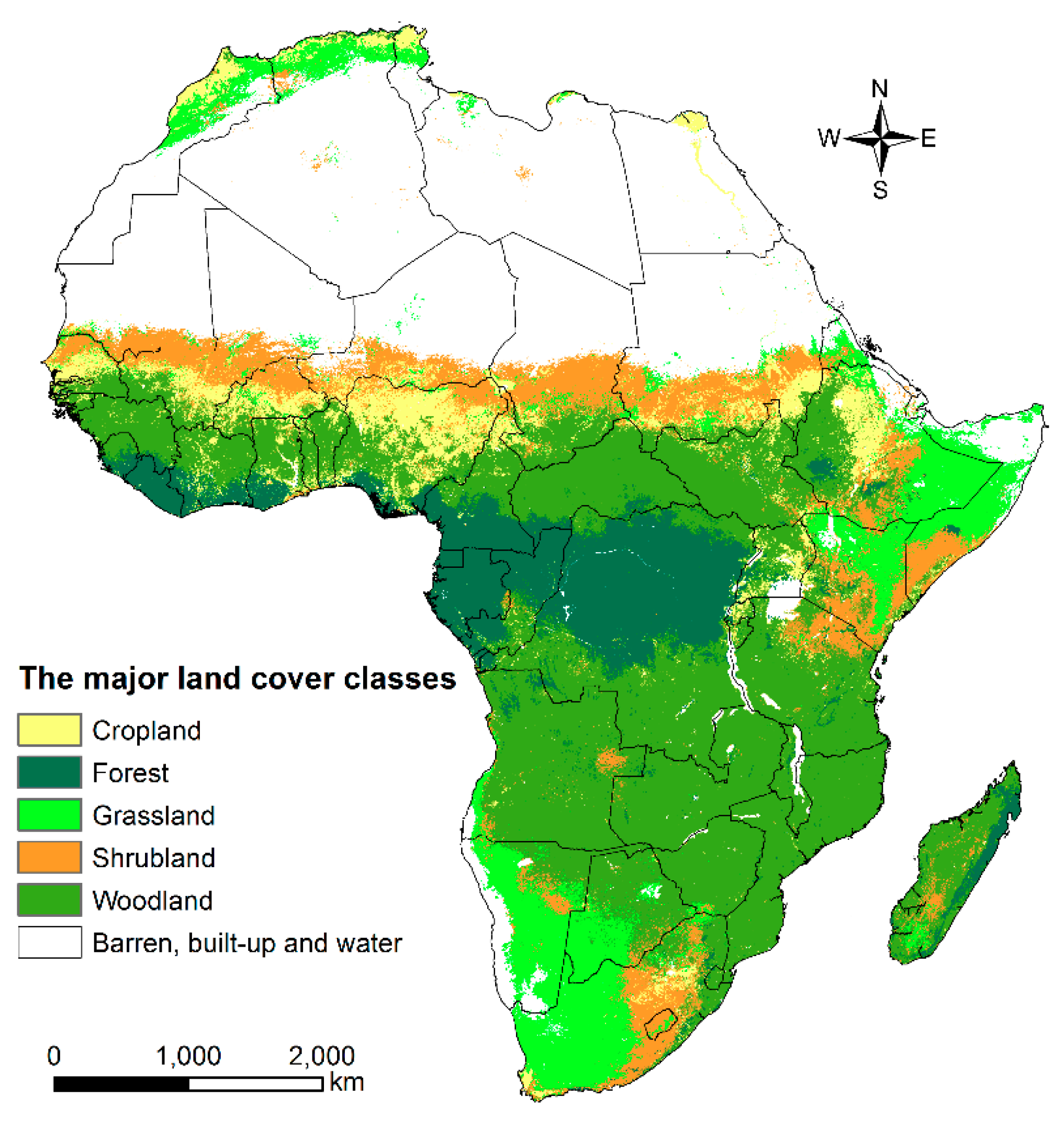
2.1. Study Area and Data

The study area encompasses the vegetative region of Africa, as shown by the land cover map in Figure 1. Monthly time series of the Enhanced Vegetation Index (EVI), precipitation, soil moisture, and GRACE TWS were used in this study (

Table 1. General description of the research data.

	Data	Resolution	Source/Citation
EVI	MODIS Collection 6 monthly EVI Product-MOD13C2: 2002–2015	~0.05°	National Aeronautics and Space Administration’s Earthdata portal (ftp://ladsweb.nascom.nasa.gov, last accessed July 2017). Didan [13]
Precipitation	CHIRPS Version 2 monthly precipitation data: 2002–2015	~5 km	Climate Hazards Group InfraRed Precipitation with Station data (CHIRPS) portal (http://chg.geog.ucsb.edu/data/chirps, last accessed July 2017). Funk et al. [14]
Soil moisture	ESA CCI daily soil moisture	~0.25°	European Space Agency Climate Change Initiative data portal (http://www.esa-soilmoisture-cci.org, last assessed July 2017). EODC [15]
Terrestrial Water Storage Anomaly (TWSA)	GRACE monthly TWSA	~1°	National Aeronautics and Space Administration’s GRACE data portal (http://grace.jpl.nasa.gov, last accessed July 2017). Swenson and Wahr [16]; Landerer and Swenson [17].

). Because GRACE TWS was first available in 2002 and we are interested in vegetation delayed response of up to 12 months to water availability (see Section 2.3), the data span of available hydrological variables that was considered was from 2002 to 2015, whereas EVI was from 2003 to 2015. Thus, the latter period determined the temporal extent of the analysis.

EVI, as a surrogate for vegetation greenness, has the advantages of being robust against background and atmospheric noises, and, unlike the Normalized Difference Vegetation Index, it does not saturate over high biomass regions [18]. For this study, EVI time series from the MOD13C2 (version 6) product, which is a derivative of image acquisitions from the moderate resolution imaging spectroradiometer (MODIS) sensor onboard the Terra satellite, was retrieved. MOD13C2 was derived from the MOD13A2 product, which is a 16-day composite at a 1-km spatial resolution.

Monthly precipitation data were obtained from the Climate Hazards Group InfraRed Precipitation with Station data portal. CHIRPS are global, gridded precipitation datasets, derived from a blend of satellite-observed infrared cold cloud duration and in situ gauge records [14]. The blending is performed using a series of algorithms and interpolation techniques, which are described in Funk et al. [14]. Validation of CHIRPS estimates against independent ground observations and some global gridded precipitation products show CHIRPS to have a relatively low bias [14]. Further, with a spatial resolution of 0.05°, CHIRPS has one of the finest spatial resolution of all the currently available long-term, global gridded precipitation products. The products, as an integral component of the Famine Early Warning Systems Network, have been used for other applications as well, e.g., [12].

Daily satellite observed soil moisture data were downloaded from the European Space Agency Climate Change Initiative data portal. The merged product comprising retrievals from the active and passive microwave soil moisture was used. This product represents the surface soil moisture not deeper than 10 cm [19]. While the merging approach is described in Liu et al. [19,20] and Wagner et al. [21] and the global validation with ground measurements is reported in Dorigo et al. [22], the merging approach used in version 03.2 (this was used for this study) includes a weighted averaging technique where the weights are proportional to the signal-to-noise ratio [15]. As this study is at a monthly time step, we averaged the original daily observations into monthly values. However, the tropical forest areas are masked out in this dataset [19] because of the difficulty of measuring soil moisture over dense vegetation with microwave remote sensing [23]. We noted a number of gridded soil moisture products with complete coverage of Africa, e.g., [24], but the soil moisture estimates are modeled from other variables, including precipitation. Thus, we opted for the microwave satellite soil moisture product, which is an independent set of measurements.

The GRACE system is made up of two satellites orbiting at identical orbital paths separated at a distance of ~220 km [25]. GRACE provides monthly measurements of the Earth’s gravity field variations, as a function of local landmasses. After accounting for atmosphere and ocean effects [26], and taking into cognizance the relatively low contribution of vegetation biomass variations [27], the net mass variation can be attributed to the redistribution of TWS. Thus, TWS is an integral of surface water, soil moisture, and groundwater. In this study, we used an ensemble of average TWS from April 2002 to December 2015 computed from the GRACE data (release-5, level-2) independently pre-processed by three research centers (NASA Jet Propulsion Laboratory (JPL), University of Texas Center for Space Research (CSR), and the GeoForschungsZentrum (GFZ) Potsdam). However, GRACE’s original signal is lost during pre-processing (e.g., filtering, de-stripping, and truncation). Hence, it is important that an appropriate scaling factor is applied to restore the signal loss prior to using water-related GRACE-TWS applications. For this reason, the scaling factor from the NCAR’s Community Land Model 4.0 (CLM4.0, [28]) was applied to correct and restore the GRACE original signal. Besides, CLM4.0 takes into account the interaction between surface and groundwater in addition to accounting for human activities such as irrigation and river diversion [17,28,29]. Consequently, the TWS used in this study is measured in equivalent water height (EWH, in cm) at a spatial resolution of 1° and at a monthly time step. In order to match the January 2002 starting point of the soil moisture and precipitation datasets, the GRACE data was extended backward by replacing the three missing months (January, February, and March) with their long-term means. It is not expected that this data interpolation will have a significant impact on the result of this study. It is worth mentioning that the GRACE-TWS was derived from subtracting the monthly observations from a historical mean (2004–2009), the output of which is commonly referred to as terrestrial water storage anomalies (TWSA) in the GRACE user community.

The soil moisture, precipitation, and the GRACE datasets were resampled to co-register with the MODIS EVI data. Each pixel of the soil moisture (0.25°) and GRACE (1°) datasets were first disaggregated to 0.05° and then resampled by the nearest neighbor technique and then aligned to the EVI dataset. These two approaches ensure minimum loss of information in the downscaling process. However, the CHIRPS pixels were only resampled to match the MODIS EVI pixels using the nearest neighbor approach. The two-step (disaggregation and nearest neighbor interpolation) approach used here replicates the pixels without necessarily altering the original cell values.

We masked some pixels based on the following considerations. Any pixel missing more than 20% of data or where there are more than three consecutive months of missing data was masked out. Otherwise, we filled the missing values using a spline interpolation algorithm [30]. Furthermore, to focus the analysis on vegetated areas, pixels with time series having a mean EVI not exceeding 0.1 were masked out. EVI values below this threshold are indicative of bare soil or open water bodies [31].

A key focus of this study is to understand the relative importance of the hydrological measures as drivers of vegetation greenness, based on original and anomalies values. For this reason, monthly anomalies were computed by subtracting the climatology (long-term mean) of each calendar month from the corresponding monthly time series over the years covered in this study. The equation for this is given by

$$X_{anomaly}\left(i,j\right)=X\left(i,j\right)-\frac{1}{n}{\displaystyle \sum }_{j=1}^{n}X\left(i,j\right),$$

(1)

where X is the monthly observed variable, i is the month, j is the year, and n is the number of the years of the data. It should be noted that for the GRACE data, the computed monthly anomaly should not be confused with the original GRACE data in which the long-term mean has been subtracted and is referred to as TWSA. To avoid confusion, the original GRACE data will still be referred to as TWSA in this paper.

2.2. Trend Analysis

Trend analysis was performed on the time series of the monthly anomalies of each of the variables: EVI, precipitation, soil moisture, and TWSA over the period 2003 to 2015. The trend was estimated using the Mann–Kendell (MK) trend test [32,33]. The MK test evaluates a series for the presence and persistence of monotonic trend (increase/decrease) through pairwise comparison of observations. The test outputs Kendall’s tau rank correlation coefficients (τ), which takes on values between −1 and 1 [33]. Positive, zero, or negative τ values, respectively, indicate an increasing, no trend, or a decreasing trend. The test is non-parametric and is widely used in remote sensing time series analysis, e.g., [12]. The MK test was used in this study because of its robustness to outliers and its capacity to handle short or noisy series compared to parametric tests such as ordinary least squares regression. Finally, only Kendall’s τ values where the estimated trend was significantly different from zero (p < 0.05) were retained.

2.3. Modeling the Relationship between Vegetation Greenness Dynamics and Water Availability

In cognizance of the possible vegetation response to water availability exhibiting time lags, the relationship between vegetation greenness and the water availability was estimated with EVI as the response variable and 0–6 and 12 months lagged measures of the hydrological variables as predictors. Consequently, the time series of EVI for the period 2003 to 2015 was used, whereas the predictor variables were drawn from the time series of the hydrological variables covering the period from 2002 to 2015. This resulted in 156 observations for each pixel for the response and the 24 predictor variables (3 variables × 8 lags).

The relationship between EVI and the hydrological measures at the associated lags was estimated with random forest (RF). We chose to use RF because it is a distribution-free, non-parametric algorithm that can be used to model simple and complex relationships between response and predictor variables [7]. It has been widely used in many regression and classification problems [34,35]. In addition to being robust in the presence of irrelevant features, RF estimates a metric for the relative importance of the predictor variables to the prediction problem [7]. The variable importance (VIP) metric indicates the decrease in prediction accuracy on an out-of-bag sample (test sample) in which the values of a variable are randomly reshuffled as against the prediction accuracy on the same out-of-bag sample with no reshuffle. The higher the decrease in prediction accuracy, the more is the predictive power of the variable in the model. In this study, the RF model was estimated for each pixel with the number of trees set to 500, above which there is no significant improvement of model performance. The default values for the other parameters (e.g., mtry and node size) in the R statistical software implementation of RF were used.

Model performance assessment: The strength of the model was assessed by comparing the out-of-bag prediction of EVI against the observed values. The comparison was based on Lin’s concordance correlation coefficient (LCCC) metric [36]. LCCC expresses the degree of agreement between the predicted values with the observed values, with respect to the 1:1 line [36].

3. Results

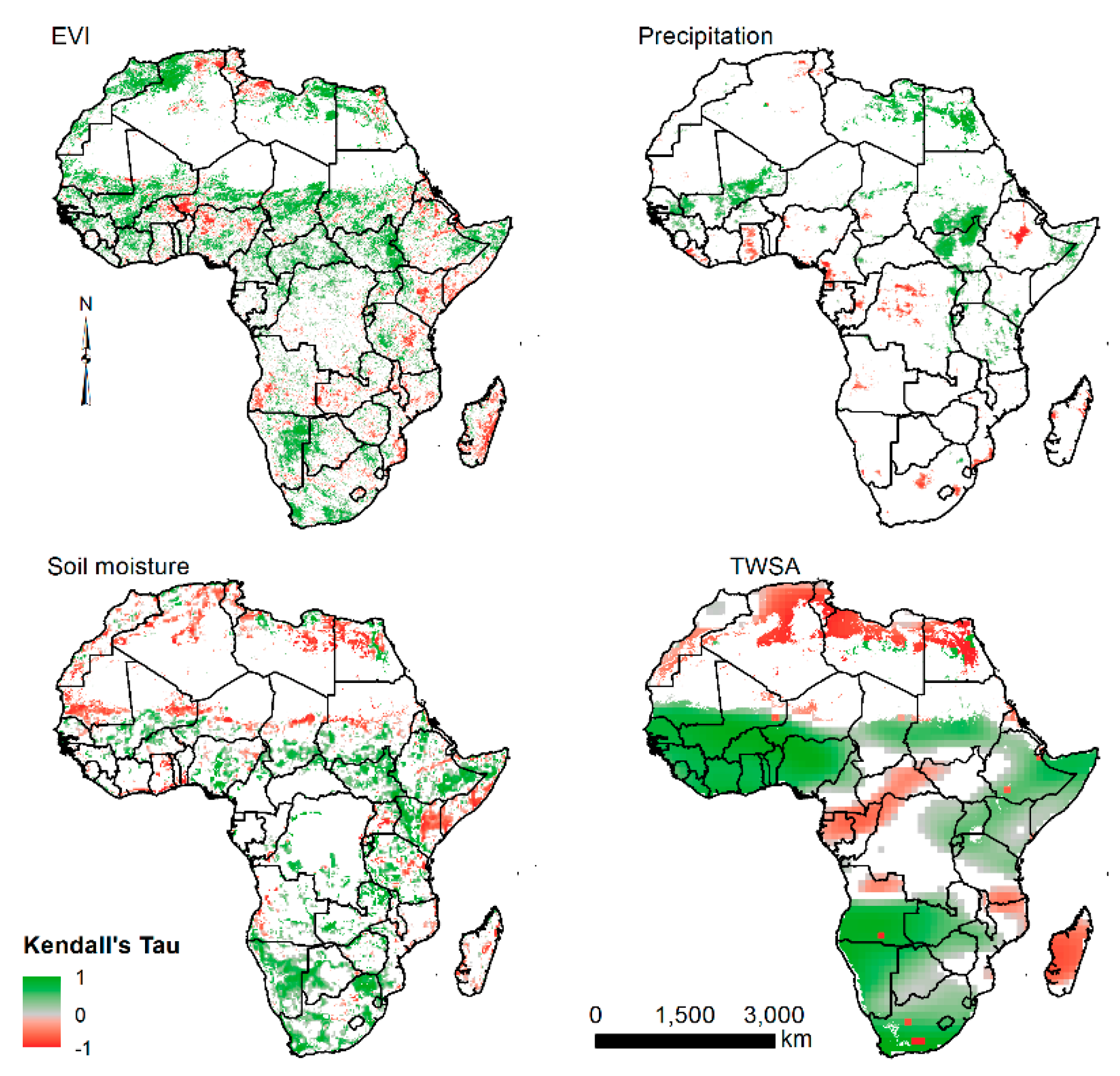
3.1. General Trends in EVI, Soil Moisture, TWSA, and Precipitation

Broadly speaking, there was a dominant positive trend in vegetation greenness anomalies in most parts of Africa (Figure 2) over the study period. Nonetheless, large clusters of a negative trend in greenness anomalies can be observed in Algeria, Tunisia, Libya, Niger, Nigeria, Ghana, Angola, and in countries in the eastern flank of Africa, extending from Eretria southwards to South Africa, and eastwards to Madagascar. Interestingly, the trajectories of vegetation greenness anomalies spatially coincided with trends in one or more of the hydrological variables in some locations. For example, the positive trend in greenness anomalies in southern Mali, in the region around the Sudan/South Sudanese border, and in parts of Angola and South Africa, is matched by an upward trend in at least two of the hydrological variables. However, a diverging direction of anomalies trends between vegetation and particularly soil moisture and TWSA, can be observed in Libya, Egypt, and also in Zambia. Finally, an important trend of ecological note is the pronounced clusters of a negative trend in precipitation and TWSA anomalies in parts of the Congo Basin.

3.2. Relationship between Vegetation Greenness Dynamics and Water Availability

Figure 3 shows the maps indicating the strength of the relationship between vegetation greenness and the hydrological variables and their lags as modeled with values of original observations (Figure 3A) and those of the monthly anomalies (Figure 3B). In the case of the original values, the relationship was very strong for most of Africa (LCCC > 0.75), although moderate relationships (LCCC = 0.5–0.75) were observed in Somalia, parts of Ethiopia and Kenya, southern Namibia, and Western South Africa, and in the northern margins of the Sahel. On the other hand, anomalies in vegetation greenness were generally less coupled to anomalies in water availability in many parts of Africa (LCCC < 0.25), notably in areas quite north of the Equator, predominantly across the savanna zones from west Senegal to the east coast of Eretria and Djibouti. However, in Namibia, Botswana, Kenya, Somalia and parts of Tanzania, Ethiopia, and South Africa, a moderate relationship between anomalies in vegetation greenness and water availability was evident (LCCC = 0.5–0.75).

Figure 4 summarizes the relationship between vegetation greenness and the hydrological variables and their lags across the major land cover types. Again, the relationship was stronger for all land cover types in the case of original values (Figure 4A) in comparison to the anomalies (Figure 4B). Furthermore, relative to the other land cover types, the relationship was generally stronger in the woodlands and croplands with the original values, whereas vegetation greenness anomalies were more coupled with anomalies in water availability in the grasslands than in the other land cover types. Regardless of which data type (original or anomaly values) was used, vegetation greenness in the forest class was relatively less associated with water availability than in the other land cover types (Figure 4A,B).

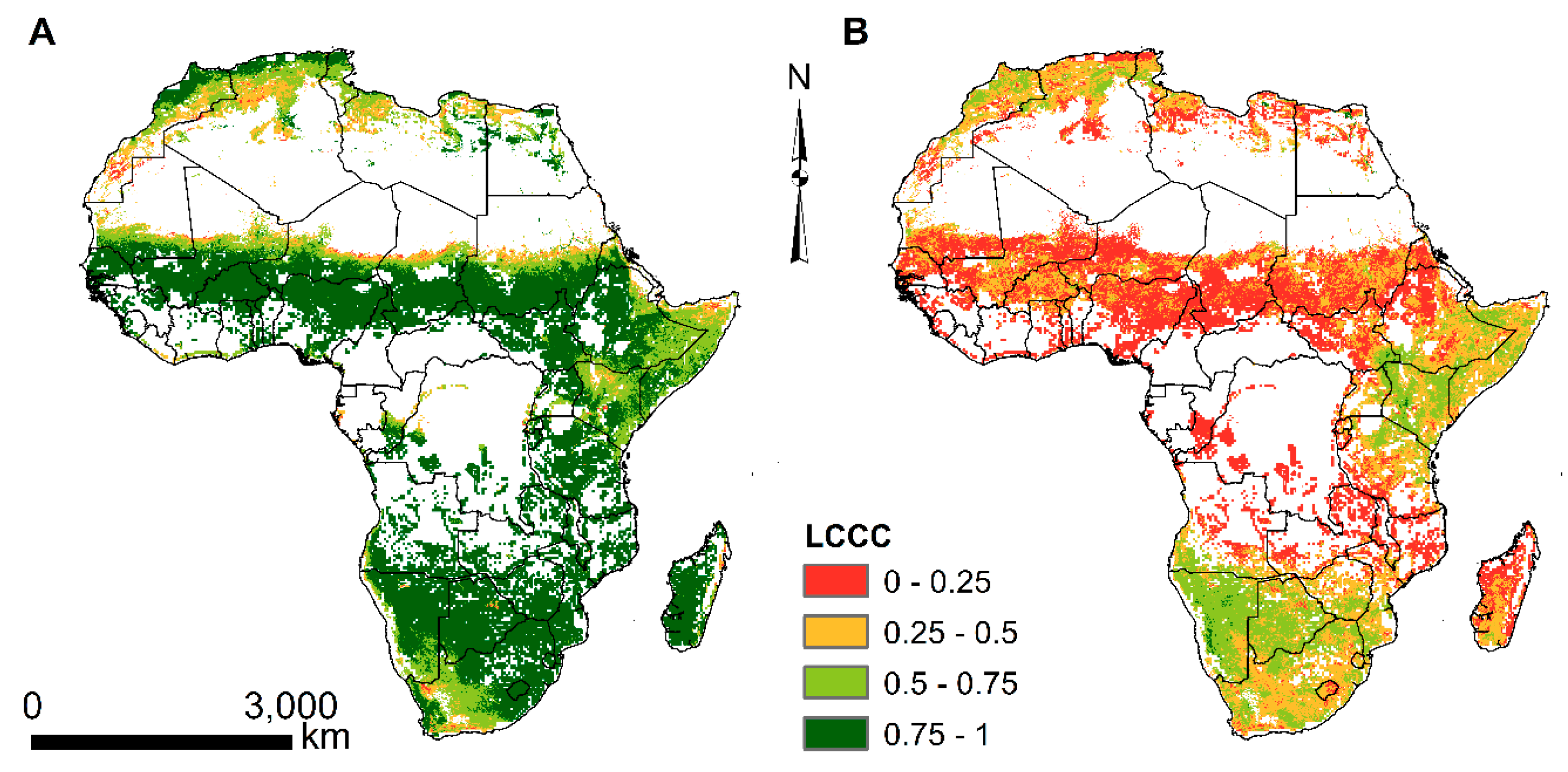
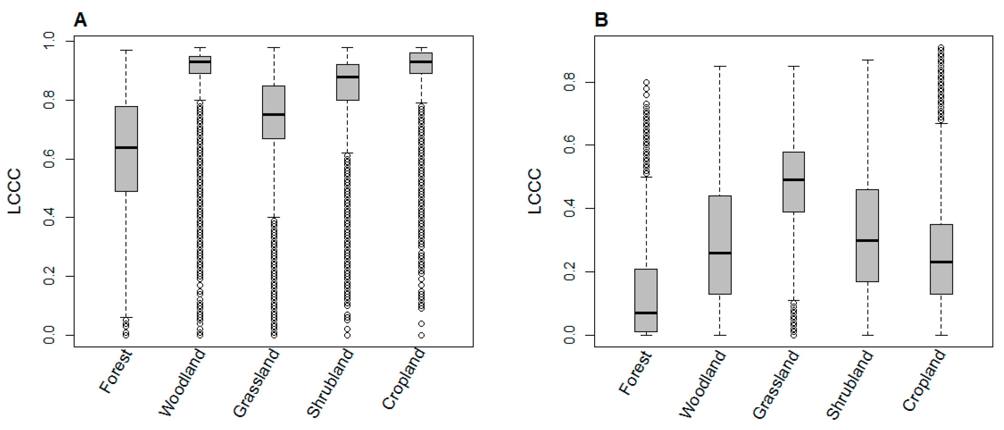
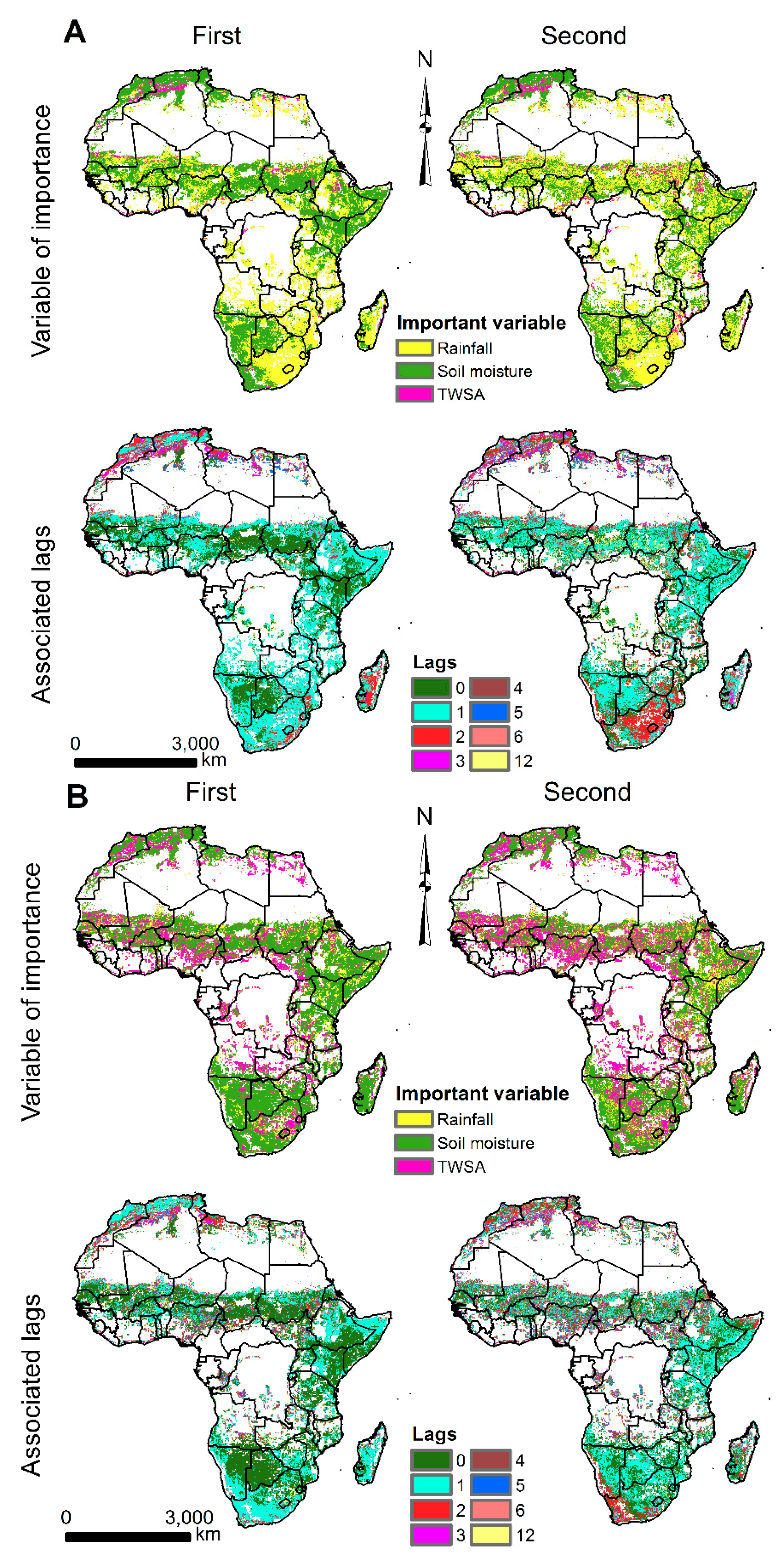
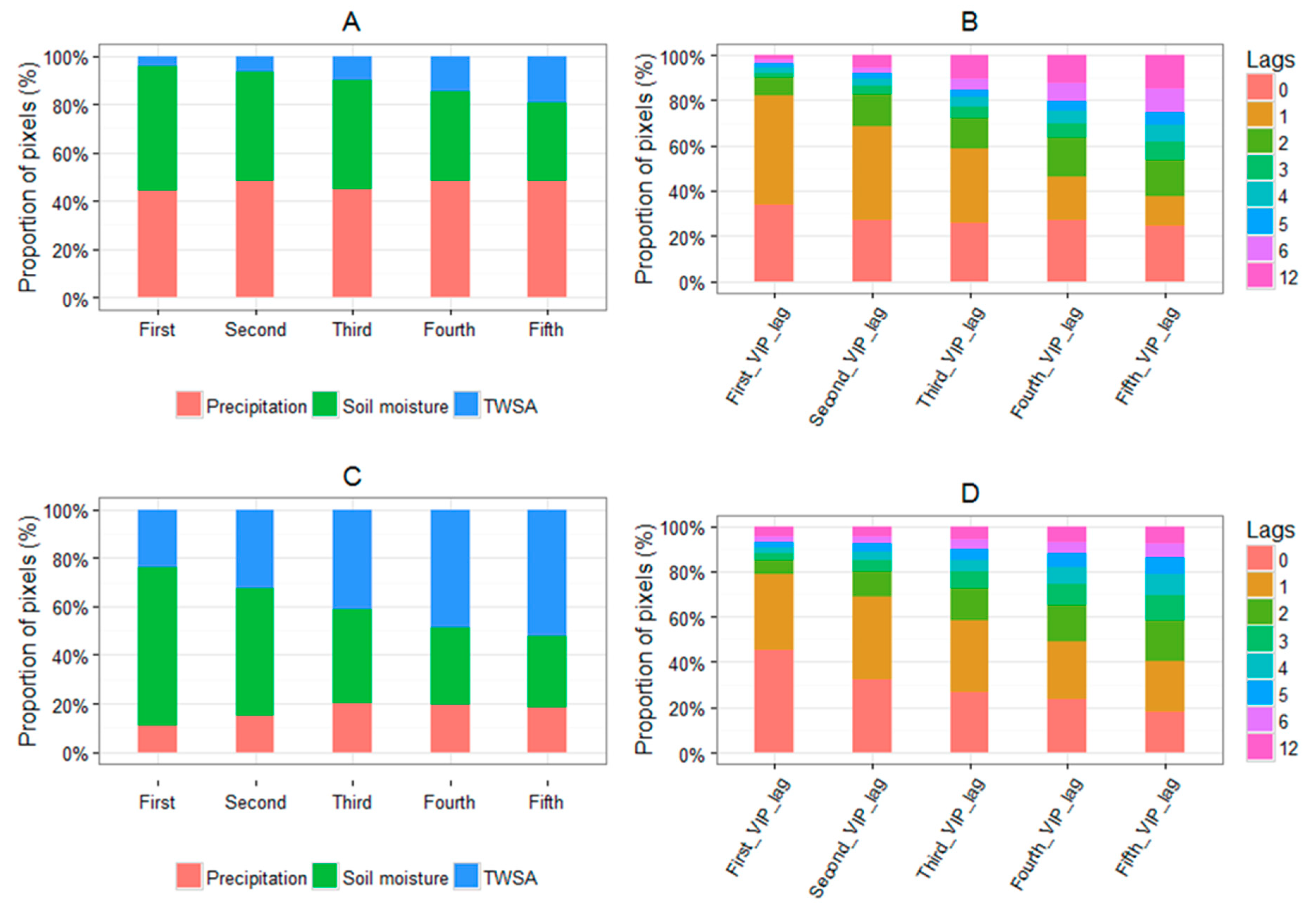
3.3. Relative Importance of Soil Moisture, Precipitation, and TWSA as Drivers of Vegetation Greenness Dynamics

Figure 5 shows the two top-ranked predictor variables and their associated lags from the modeled relationship between vegetation greenness and water availability for the original (Figure 5A) and monthly anomalies (Figure 5B) data. Figure 6 further illustrates the proportion of pixels across the five top-ranked predictors. Based on the original observations, precipitation and soil moisture were the most important predictors of vegetation greenness. The proportion of pixels where soil moisture was ranked as the topmost VIP in predicting vegetation greenness was about 55% (Figure 6A). This encompassed parts of west southern Africa, East Africa, and the western Maghreb (Figure 5A). However, the proportion rapidly declined to about 30% in the fifth VIP. Precipitation, on the other hand, was the most important hydrological variable driving vegetation greenness in the eastern flank of southern Africa (Figure 5A). The proportion of pixels across Africa where precipitation was ranked among the top five VIP was fairly constant (45%, Figure 6A). In terms of vegetation lag response to the hydrological variables, and based on the first two important predictors, precipitation generally led vegetation greenness by 1 to 2 months (e.g., in eastern South Africa), whereas soil moisture was more concurrent with or led vegetation greenness by 1 month (e.g., in Namibia and Botswana).

Anomalies in soil moisture and TWSA were the dominant hydrological predictors of anomalies in vegetation greenness in most of Africa, with the role of precipitation greatly diminished (Figure 6C). Whereas soil moisture anomalies drive anomalies in vegetation greenness in virtually all parts of Africa, anomalies in TWSA were more coupled to vegetation dynamics anomalies in the humid savanna zone of Nigeria and the semi-arid region of Egypt (Figure 5B). Nonetheless, the proportion of pixels with dominant soil moisture control of vegetation greenness anomalies decreased considerably from the first (65%) to the fifth (30%) ranked VIP. This is in contrast to that of TWSA that increased from 25% to 50% (Figure 6D). Going by the first and second VIP results, vegetation anomalies lagged precipitation and TWSA anomalies by 0 to 1 month, though the response was much delayed in some parts of North Africa (Figure 5B).

4. Discussion

4.1. Trends in EVI and the Hydrological Variables

Some of the observed trends in vegetation greenness in this study are consistent with those reported by more recent regional and continental studies. For example, the positive trend in vegetation greenness observed in most parts of the Sahel has also been reported in recent studies by Leroux et al. [37], which examined vegetation changes in the Sahel between 2000 and 2015, and by Ugbaje et al. [12], which investigated the variability of vegetation productivity across Africa between 2000 and 2014. Additionally, the hotspot of declining vegetation greenness observed in southwestern Niger is consistent with findings from many studies (e.g., [37,38]). This hotspot has been dubbed “a Sahelian exception” because it stands in contrast to the dominant Sahelian greening [37]. Likewise, the negative trend in greenness over Zambia is in line with the reported decline in vegetation productivity by Ugbaje et al. [12] for the period between 2000 and 2014. Similarly, the clusters of a negative trend in vegetation greenness in parts of Somalia, Kenya, and Tanzania correspond to those reported by [39] over the period 2000 to 2010. This indicates that vegetation activity in this region has continued to decline even after 2010, up to 2015, as reported here.

Similar to the observed vegetation greenness trends, some of the trajectories of hydrological variables are in line with those of other studies. For instance, the positive trend in soil moisture and precipitation in southern Chad and South Sudan was also reported in a study by Huber et al. [9] which analyzed vegetation greenness dynamics in relation to water availability in the Sahel over the period of 1982 to 2007. Similarly, the general positive trend in soil moisture in southern Africa is in agreement with the improvement in soil water content for the period of 1993 to 2012, observed by Wei et al. [40]. Thus, our results indicate that this positive trend in soil moisture and precipitation persisted up to 2015. Also, the observed decline in precipitation and TWSA in parts of the Congo basin has also been reported by Zhou et al. [41] for the period covering 2000 to 2012.

However, the results here show a few notable areas of differences in trend directions from what is reported by other studies. For example, in Ugbaje et al. [12], vegetation productivity in Angola was largely stable, which is in contrast with a dominant positive trend in vegetation greenness observed in this study (Figure 2). Similarly, contrary to Zhou et al. [41] who observed a corresponding decrease in EVI following a decline in water availability in the Congo, here, EVI for most parts of the basin was either stable or showed a positive trend (Figure 2). This may be due to improvement in non-water related constraints like decreasing cloud cover and the concomitant increase in solar radiation [42]. Overall, the differences in the trajectories of vegetation dynamics between these studies and those in this study may be linked to the contrast in the time interval considered for the trend analyses.

4.2. Spatiotemporal Variation of Vegetation Greenness in Relation to Water Availability

Unlike many studies that assessed the relationship of vegetation greenness and water availability using one or more hydrological variables from remote sensing (e.g., [3,6,43]), this is the first study, to the best of our knowledge, that has analyzed vegetation greenness dynamics in relation to precipitation, soil moisture, and TWSA within a multivariate framework. The RF modeling results of water availability were generally strongly coupled to vegetation greenness when the cyclic seasonal variation in the analyzed time series is not removed. This is generally expected for Africa as the vegetation phenological cycle is primarily driven by the wet–dry season cycle. However, the moderate relationship observed in the semi-arid areas like in the Horn of Africa and the northern Sahel can be explained by their erratic precipitation regime.

On the flip side, when the monthly means were removed from the time series, the strong relationships between vegetation greenness and water availability was not as widespread across Africa. Most notably, the observed relationship was weak in the savanna belt stretching from the West coast of Africa to the east coast of Eretria and Djibouti. This result implies that the predominantly positive trend in greenness anomalies observed in the region may be driven by factors other than water availability. Such factors may include atmospheric fertilization, agricultural intensification including the use of improved and high yielding crop cultivars, afforestation, and a positive trend in the growing season length [44,45,46]. However, in eastern and southern Africa, south of Zambia, vegetation greenness anomaly dynamics was more linked to anomalies in water availability compared to the relationship observed in West Africa across to the east coast of Eretria and Djibouti. The relatively high proportion of grass cover in most parts of eastern and southern Africa (see Figure 1) may, in part, explain this difference in regional response to water availability. Because of their shallow rooting system, grasses are generally more sensitive to fluctuations in near-surface soil moisture availability than most woody plants [47], as can be seen from the relatively strong relationship obtained for the grassland cover type (Figure 4B). Nonetheless, the sensitivity of grassland linked to moisture anomalies is also a reflection of the increasing frequency and severity of water-related extreme events such as drought and flooding in eastern and southern Africa [48,49]. Therefore, the dynamics in water availability related to anomalies in one or more of the hydrological variables (soil moisture, TWSA, and rainfall) was to a large extent the principal driver of trends in vegetation greenness anomalies observed in eastern and southern Africa.

4.3. The Relative Roles of Precipitation, Soil Moisture and TWSA in Driving Vegetation Greenness

The dominance of soil moisture as the first ranked predictor of vegetation greenness dynamics in substantial parts of Africa from the two RF models (original or monthly anomalies data) (Figure 5) can be attributed to soil moisture being a better integral of the effects of topography and energy on plant available water than precipitation and TWSA. This also confirms soil moisture as a vital component of the hydrological cycle better linked with the vegetation phenological cycle [8]. However, there are locations where precipitation and/or TWSA were better indicators of plant available water than soil moisture. For example, with the original data, precipitation outranked soil moisture (and TSWA) as a predictor of vegetation greenness dynamics in south-eastern Africa which contrasts with south-western Africa where soil moisture exercised dominant control (Figure 5A). The better performance of precipitation in south-eastern Africa can be attributed to the strong influence of the adjacent Indian Ocean and ENSO events on the ecohydrological regime of the area [50].

Although precipitation is considered the primary climatic driver of vegetation phenology [8], here monthly anomalies of precipitation were not as important as anomalies in soil moisture and TWSA in explaining anomalies in vegetation canopy greening across Africa. This result is similar to the findings in other studies that reported a better correlation between satellite-observed soil moisture and NDVI anomalies (e.g., [4]) and between GRACE TWSA and NDVI anomalies (e.g., [6]). This result, therefore, is in line with the understanding that the amount of water stored in the soil rather than the amount of precipitation received determines the survival of plants to extreme events like drought.

Regardless of whether the original or anomalies time series was used for modeling, vegetation greenness generally responded quicker (0–1 months) to changes in soil moisture and TWSA than to precipitation (1–2 months). This is plausible especially if we consider precipitation as the source and soil moisture and TWSA as the conduit of plant-available water. This premise is also supported by the results of Chen et al. [4] and Yang et al. [6] which indicated a generally strong correlation between vegetation greenness anomalies and soil moisture and TWSA anomalies over Australia at 0 to 1 months of vegetation delayed response. On the global scale, Xie et al. [51] also observed a vegetation greenness delayed response of 0- to 1-month to the TWSA. Additionally, Yang et al. [6] and Gessner et al. [3] found NDVI to be strongly correlated with precipitation at time lags upwards of a month.

5. Conclusions and Outlook

Remote sensing observations of EVI, soil moisture, TWSA, and station-satellite blend precipitation products were used to assess the impact/influence of the hydrological controls of vegetation greenness dynamics over Africa for the period between 2003 and 2015. By using a multivariate approach with the distribution-free RF algorithm, the relationships between these hydrological variables and vegetation greenness, with and without monthly anomalies, were assessed. The advantage of this approach is that it allows for the modeling of complex interactions between vegetation greenness and the hydrological variables, including lag effects. This is a more robust way to assess the relative importance of the hydrological variables and their lag effects on vegetation response to water availability.

In most parts of Africa, the RF model with the seasonal component present in the time series (original data) generally performed better than the model driven by monthly anomalies of the variables. These results indicate that water availability is a better driver of vegetation phenology than anomalous vegetation greenness trends in most parts of Africa. This contrast in model performance is particularly striking across West Africa and eastward to Eretria and Djibouti. With regards to the relative importance of the three hydrological variables to vegetation greenness dynamics, soil moisture was the only variable that consistently performed with both time series types and was ranked as the first important variable in more than 50% of the pixels examined. Nonetheless, precipitation and TWSA had significant roles in controlling vegetation greenness with the original and monthly anomaly time series, respectively. Of particular note is the strong predictive power of precipitation in the eastern flank of south-eastern Africa, which is a demonstration of the strong influence of the adjacent Indian Ocean on the vegetation dynamics of the region. In terms of the response of vegetation greenness to changes in the hydrological measure, soil moisture, and TWSA were generally concurrent or led vegetation by 1 month, whereas precipitation led vegetation by 1–2 months. This demonstrates that soil moisture and TWSA are direct indicators of plant-available water than precipitation.

However, a key point to note is that soil moisture may have masked the strength of TWSA in predicting vegetation greenness response to water since TWSA is a measure of water stored from the surface to the boundary between the earth’s crust and the mantle, which is inclusive of soil moisture. The soil moisture product used in this study represents measurements not deeper than 10 cm. This relationship between soil moisture and TWSA explains why the total area where soil moisture was important rapidly declined with a concomitant increase in the total area of TWSA influence across the variable of importance ranking (Figure 6). Thus, there is the need to further partition GRACE TWSA into the surface and groundwater components. However, because the current microwave sensors measure only soil moisture at the top few centimeters, TWSA supplements these measurements in areas where the root zone is deeper. Another possibility is to jointly assimilate the SMOS near-surface soil moisture observations and TWSA into a hydrological model to better approximate the root zone soil moisture, as demonstrated recently by Tian et al. [47], providing a better indicator of plant-available water and better vegetation response.

All in all, our results illustrate the usefulness of remote sensing soil moisture and TWSA as complementary data to precipitation in assessing and monitoring vegetation greenness dynamics, despite their relatively low spatial resolution (>0.25°). This is especially important in Africa, where there is a dearth of in situ precipitation and soil moisture observations. Furthermore, the relationships observed across the vegetation types in this study can be used in benchmarking coupled vegetation-climate models. The generally low correlation between vegetation greenness anomalies and the hydrological variables anomalies observed over most of Africa (Figure 3B) can be improved if additional hydroclimatic variables such as vapor pressure deficit and evapotranspiration, as well as root zone soil moisture estimates, are incorporated to the RF model.

References

1. Heimann, M.; Reichstein, M. Terrestrial ecosystem carbon dynamics and climate feedbacks. Nature 2008, 451, 289–292. [Google Scholar] [CrossRef] [PubMed]
2. Herrmann, S.M.; Anyamba, A.; Tucker, C.J. Recent trends in vegetation dynamics in the African Sahel and their relationship to climate. Glob. Environ. Chang. 2005, 15, 394–404. [Google Scholar] [CrossRef]
3. Gessner, U.; Naeimi, V.; Klein, I.; Kuenzer, C.; Klein, D.; Dech, S. The relationship between precipitation anomalies and satellite-derived vegetation activity in Central Asia. Glob. Planet. Chang. 2013, 110, 74–87. [Google Scholar] [CrossRef]
4. Chen, T.; McVicar, T.R.; Wang, G.; Chen, X.; De Jeu, R.A.M.; Liu, Y.Y.; Shen, H.; Zhang, F.; Dolman, A.J. Advantages of using microwave satellite soil moisture over gridded precipitation products and land surface model output in assessing regional vegetation water availability and growth dynamics for a lateral inflow receiving landscape. Remote Sens. 2016, 8, 428. [Google Scholar] [CrossRef] [Green Version]
5. Ndehedehe, C.E.; Ferreira, V.G.; Agutu, N.O. Hydrological controls on surface vegetation dynamics over West and Central Africa. Ecol. Indic. 2019, 103, 494–508. [Google Scholar] [CrossRef]
6. Yang, Y.; Long, D.; Guan, H.; Scanlon, B.R.; Simmons, C.T.; Jiang, L.; Xu, X. GRACE satellite observed hydrological controls on interannual and seasonal variability in surface greenness over mainland Australia. J. Geophys. Res. Biogeosci. 2014, 119, 2245–2260. [Google Scholar] [CrossRef]
7. Breiman, L. Random forests. Mach. Learn. 2001, 45, 5–32. [Google Scholar] [CrossRef] [Green Version]
8. Stampoulis, D.; Andreadis, K.M.; Granger, S.L.; Fisher, J.B.; Turk, F.J.; Behrangi, A.; Ines, A.V.; Das, N.N. Assessing hydro-ecological vulnerability using microwave radiometric measurements from WindSat. Remote Sens. Environ. 2016, 184, 58–72. [Google Scholar] [CrossRef]
9. Huber, S.; Fensholt, R.; Rasmussen, K. Water availability as the driver of vegetation dynamics in the African Sahel from 1982 to 2007. Glob. Planet. Chang. 2011, 76, 186–195. [Google Scholar] [CrossRef]
10. Campo-Bescós, M.; Muñoz-Carpena, R.; Southworth, J.; Zhu, L.; Waylen, P.; Bunting, E. Combined Spatial and Temporal Effects of Environmental Controls on Long-Term Monthly NDVI in the Southern Africa Savanna. Remote Sens. 2013, 5, 6513–6538. [Google Scholar] [CrossRef] [Green Version]
11. Farrar, T.J.; Nicholson, S.E.; Lare, A.R. The influence of soil type on the relationships between NDVI, rainfall, and soil moisture in semiarid Botswana. II. NDVI response to soil moisture. Remote Sens. Environ. 1994, 133, 121–133. [Google Scholar] [CrossRef]
12. Ugbaje, S.U.; Odeh, I.O.A.; Bishop, T.F.A.; Li, J. Assessing the spatio-temporal variability of vegetation productivity in Africa: Quantifying the relative roles of climate variability and human activities. Int. J. Digit. Earth 2017, 10, 879–900. [Google Scholar] [CrossRef]
13. Didan, K. MOD13C2 MODIS/Terra Vegetation Indices Monthly L3 Global 0.05Deg CMG V006. 2015. Available online: https://lpdaac.usgs.gov/products/mod13c2v006/ (accessed on 31 July 2017).
14. Funk, C.; Peterson, P.; Landsfeld, M.; Pedreros, D.; Verdin, J.; Shukla, S.; Husak, G.; Rowland, J.; Harrison, L.; Hoell, A.; et al. The climate hazards infrared precipitation with stations—A new environmental record for monitoring extremes. Sci. Data 2015, 2, 150066. [Google Scholar] [CrossRef] [PubMed] [Green Version]
15. EODC Product Specification Document (D1.2.1 Version 1.9). Available online: http://www.esa-soilmoisture-cci.org/sites/default/files/documents/ESA_CCI_SM_PSD_D1.2.1_v1.9.pdf (accessed on 1 July 2017).
16. Swenson, S.; Wahr, J. Post-processing removal of correlated errors in GRACE data. Geophys. Res. Lett. 2006, 33. [Google Scholar] [CrossRef]
17. Landerer, F.W.; Swenson, S.C. Accuracy of scaled GRACE terrestrial water storage estimates. Water Resour. Res. 2012, 48. [Google Scholar] [CrossRef]
18. Huete, A.; Didan, K.; Miura, T.; Rodriguez, E.P.; Gao, X.; Ferreira, L.G. MODIS_MOD13_NDVI_referenc. 2002, 83, 195–213. Remote Sens. Environ. 2002, 83, 195–213. [Google Scholar]
19. Liu, Y.Y.; Parinussa, R.M.; Dorigo, W.A.; De Jeu, R.A.M.; Wagner, W.; Van Dijk, A.I.J.M.; McCabe, M.F.; Evans, J.P. Developing an improved soil moisture dataset by blending passive and active microwave satellite-based retrievals. Hydrol. Earth Syst. Sci. 2011, 15, 425–436. [Google Scholar] [CrossRef] [Green Version]
20. Liu, Y.Y.; Dorigo, W.A.; Parinussa, R.M.; De Jeu, R.A.M.; Wagner, W.; McCabe, M.F.; Evans, J.P.; Van Dijk, A.I.J.M. Trend-preserving blending of passive and active microwave soil moisture retrievals. Remote Sens. Environ. 2012, 123, 280–297. [Google Scholar] [CrossRef]
21. Wagner, W.; Dorigo, W.; de Jeu, R.; Fernandez, D.; Benveniste, J.; Haas, E.; Ertl, M. Fusion of Active and Passive Microwave Observations To Create an Essential Climate Variable Data Record on Soil Moisture. ISPRS Ann. Photogramm. Remote Sens. Spat. Inf. Sci. 2012, 7, 315–321. [Google Scholar]
22. Dorigo, W.A.; Gruber, A.; De Jeu, R.A.M.; Wagner, W.; Stacke, T.; Loew, A.; Albergel, C.; Brocca, L.; Chung, D.; Parinussa, R.M.; et al. Evaluation of the ESA CCI soil moisture product using ground-based observations. Remote Sens. Environ. 2015, 162, 380–395. [Google Scholar] [CrossRef]
23. Wagner, W.; Blöschl, G.; Pampaloni, P.; Calvet, J.-C.; Bizzarri, B.; Wigneron, J.-P.; Kerr, Y. Operational readiness of microwave remote sensing of soil moisture for hydrologic applications. Nord. Hydrol. 2007, 38, 1. [Google Scholar] [CrossRef]
24. Fan, Y.; van den Dool, H. Climate Prediction Center global monthly soil moisture data set at 0.5° resolution for 1948 to present. J. Geophys. Res. D Atmos. 2004, 109, 1–8. [Google Scholar] [CrossRef] [Green Version]
25. Rodell, M.; Famiglietti, J.S.; Chen, J.; Seneviratne, S.I.; Viterbo, P.; Holl, S.; Wilson, C.R. Basin scale estimates of evapotranspiration using GRACE and other observations. Geophys. Res. Lett. 2004, 31. [Google Scholar] [CrossRef] [Green Version]
26. Tapley, B.D. GRACE Measurements of Mass Variability in the Earth System. Science 2004, 305, 503–505. [Google Scholar] [CrossRef] [Green Version]
27. Rodell, M.; Chao, B.F.; Au, A.Y.; Kimball, J.S.; McDonald, K.C. Global biomass variation and its geodynamic effects: 1982-98. Earth Interact. 2005, 9, 1–19. [Google Scholar] [CrossRef] [Green Version]
28. Gent, P.R.; Danabasoglu, G.; Donner, L.J.; Holland, M.M.; Hunke, E.C.; Jayne, S.R.; Lawrence, D.M.; Neale, R.B.; Rasch, P.J.; Vertenstein, M.; et al. The community climate system model version 4. J. Clim. 2011, 24, 4973–4991. [Google Scholar] [CrossRef]
29. Long, D.; Longuevergne, L.; Scanlon, B.R. Global analysis of approaches for deriving total water storage changes from GRACE satellites. Water Resour. Res. 2015, 51, 2574–2594. [Google Scholar] [CrossRef] [Green Version]
30. Moritz, S.; Bartz-Beielstein, T. imputeTS: Time Series Missing Value Imputation in R. R Journal 2017, 9, 207–218. [Google Scholar] [CrossRef] [Green Version]
31. Myneni, R.B.; Williams, D.L. On the relationship between FAPAR and NDVI. Remote Sens. Environ. 1994, 49, 200–211. [Google Scholar] [CrossRef]
32. Mann, H.B. Nonparametric tests against trend. Econom. J. Econom. Soc. 1945, 13, 245–259. [Google Scholar] [CrossRef]
33. Kendall, M.G. A new measure of rank correlation. Biometrika 1938, 30, 81–93. [Google Scholar] [CrossRef]
34. Hengl, T.; Heuvelink, G.B.M.; Kempen, B.; Leenaars, J.G.B.; Walsh, M.G.; Shepherd, K.D.; Sila, A.; MacMillan, R.A.; De Jesus, J.M.; Tamene, L.; et al. Mapping soil properties of Africa at 250 m resolution: Random forests significantly improve current predictions. PLoS ONE 2015, 10, e0125814. [Google Scholar] [CrossRef] [PubMed]
35. Gessner, U.; Machwitz, M.; Esch, T.; Tillack, A.; Naeimi, V.; Kuenzer, C.; Dech, S. Multi-sensor mapping of West African land cover using MODIS, ASAR and TanDEM-X/TerraSAR-X data. Remote Sens. Environ. 2015, 164, 282–297. [Google Scholar] [CrossRef]
36. Lin, L.I. A concordance correlation coefficient to evaluate reproducibility. Biometrics 1989, 45, 255–268. [Google Scholar] [CrossRef]
37. Leroux, L.; Bégué, A.; Lo Seen, D.; Jolivot, A.; Kayitakire, F. Driving forces of recent vegetation changes in the Sahel: Lessons learned from regional and local level analyses. Remote Sens. Environ. 2017, 191, 38–54. [Google Scholar] [CrossRef] [Green Version]
38. Dardel, C.; Kergoat, L.; Hiernaux, P.; Mougin, E.; Grippa, M.; Tucker, C.J.J. Re-greening Sahel: 30 years of remote sensing data and field observations (Mali, Niger). Remote Sens. Environ. 2014, 140, 350–364. [Google Scholar] [CrossRef]
39. Hoscilo, A.; Balzter, H.; Bartholomé, E.; Boschetti, M.; Brivio, P.A.; Brink, A.; Clerici, M.; Pekel, J.F. A conceptual model for assessing rainfall and vegetation trends in sub-Saharan Africa from satellite data. Int. J. Climatol. 2015, 35, 3582–3592. [Google Scholar] [CrossRef] [Green Version]
40. Wei, F.; Wang, S.; Fu, B.; Wang, L.; Liu, Y.Y.; Li, Y. African dryland ecosystem changes controlled by soil water. Land Degrad. Dev. 2019, 30, 1564–1573. [Google Scholar] [CrossRef]
41. Zhou, L.; Tian, Y.; Myneni, R.B.; Ciais, P.; Saatchi, S.; Liu, Y.Y.; Piao, S.; Chen, H.; Vermote, E.F.; Song, C.; et al. Widespread decline of Congo rainforest greenness in the past decade. Nature 2014, 509, 86–90. [Google Scholar] [CrossRef]
42. Nemani, R.R.; Keeling, C.D.; Hashimoto, H.; Jolly, W.M.; Piper, S.C.; Tucker, C.J.; Myneni, R.B.; Running, S.W. Climate-driven increases in global terrestrial net primary production from 1982 to 1999. Science 2003, 300, 1560–1563. [Google Scholar] [CrossRef] [Green Version]
43. Chen, T.; de Jeu, R.A.M.; Liu, Y.Y.; van der Werf, G.R.; Dolman, A.J. Using satellite based soil moisture to quantify the water driven variability in NDVI: A case study over mainland Australia. Remote Sens. Environ. 2014, 140, 330–338. [Google Scholar] [CrossRef]
44. Boschetti, M.; Nutini, F.; Brivio, P.A.; Bartholomé, E.; Stroppiana, D.; Hoscilo, A. Identification of environmental anomaly hot spots in West Africa from time series of NDVI and rainfall. ISPRS J. Photogramm. Remote Sens. 2013, 78, 26–40. [Google Scholar] [CrossRef]
45. Vrieling, A.; de Leeuw, J.; Said, M. Length of Growing Period over Africa: Variability and Trends from 30 Years of NDVI Time Series. Remote Sens. 2013, 5, 982–1000. [Google Scholar] [CrossRef] [Green Version]
46. Pan, S.; Dangal, S.R.S.; Tao, B.; Yang, J.; Tian, H. Recent patterns of terrestrial net primary production in Africa influenced by multiple environmental changes. Ecosyst. Heal. Sustain. 2015, 1, 1–15. [Google Scholar] [CrossRef] [Green Version]
47. Tian, S.; Renzullo, L.J.; Van Dijk, A.I.J.M.; Tregoning, P.; Walker, J.P. Global joint assimilation of GRACE and SMOS for improved estimation of root-zone soil moisture and vegetation response. Hydrol. Earth Syst. Sci. 2019, 23, 1067–1081. [Google Scholar] [CrossRef] [Green Version]
48. Hooli, L.J. Resilience of the poorest: Coping strategies and indigenous knowledge of living with the floods in Northern Namibia. Reg. Environ. Chang. 2016, 16, 695–707. [Google Scholar] [CrossRef]
49. Nicholson, S.E. A detailed look at the recent drought situation in the Greater Horn of Africa. J. Arid Environ. 2014, 103, 71–79. [Google Scholar] [CrossRef]
50. Nicholson, S.E.; Kim, J. The relationship of the el nino oscillation to african rainfall. Int. J. Climatol. 1997, 17, 117–135. [Google Scholar] [CrossRef]
51. Xie, X.; He, B.; Guo, L.; Miao, C.; Zhang, Y. Detecting hotspots of interactions between vegetation greenness and terrestrial water storage using satellite observations. Remote Sens. Environ. 2019, 231, 111259. [Google Scholar] [CrossRef]
Figure 1. The major land cover types across Africa aggregated from the University of Maryland (UMD) MODIS land cover layer for 2013 (adapted from Ugbaje et al. [12]).
Land 09 00015 g001
Figure 2. Trends in anomalies of EVI, precipitation, soil moisture, and TWSA over Africa from 2003 to 2015. The white areas are either no trend (p > 0.05), barren, no data, or water bodies.
Land 09 00015 g002
Figure 3. Spatial variability of the strength (LCCC) of vegetation greenness response to concurrent and lagged precipitation, soil moisture, and TWSA for the period 2003 to 2015 based on monthly time series of (A) original observations and (B) anomalies. The white areas are masked out either due to no data, barren land, or water bodies.
Land 09 00015 g003
Figure 4. Relationship between vegetation greenness and concurrent and lagged precipitation, soil moisture, and TWSA across major land cover types for the period 2003 to 2015 based on monthly time series of (A) original observations and (B) anomalies.
Land 09 00015 g004
Figure 5. Spatial distribution of the top two ranked VIPs of the hydrological variables and their associated lags in (months) in modeling vegetation response to water availability in Africa based on monthly time series of (A) original observations and (B) anomalies. The white areas are masked out either due to no data, barren land, or water bodies.
Land 09 00015 g005
Figure 6. Summary of the first five ranked variable of importance of the hydrological variables and their lags in driving vegetation response to water availability across Africa based on (A,B) original and (C,D) anomalies monthly data.
Land 09 00015 g006