
Typologies and Spatialization of Agricultural Production Systems in Rondônia, Brazil: Linking Land Use, Socioeconomics and Territorial Configuration

 ,
,
Abstract
:1. Introduction
2. Materials and Data Preparation
2.1. Study Area
2.2. Metrics to Characterization of Production Systems
2.2.1. Dimension 1: Agricultural Production
2.2.2. Dimension 2: Economics
2.2.2.1. Gross Domestic Product (GDP)
2.2.2.2. Agricultural Credit
2.2.2.3. Logistics
2.2.3. Dimension 3: Territorial Configuration
2.2.3.1. The Amazon Deforestation Monitoring Project (PRODES)
2.2.3.2. TerraClass
2.2.3.3. Conservation Units
2.2.4. Dimension 4: Social Characteristics
3. Metrics and Data Analysis
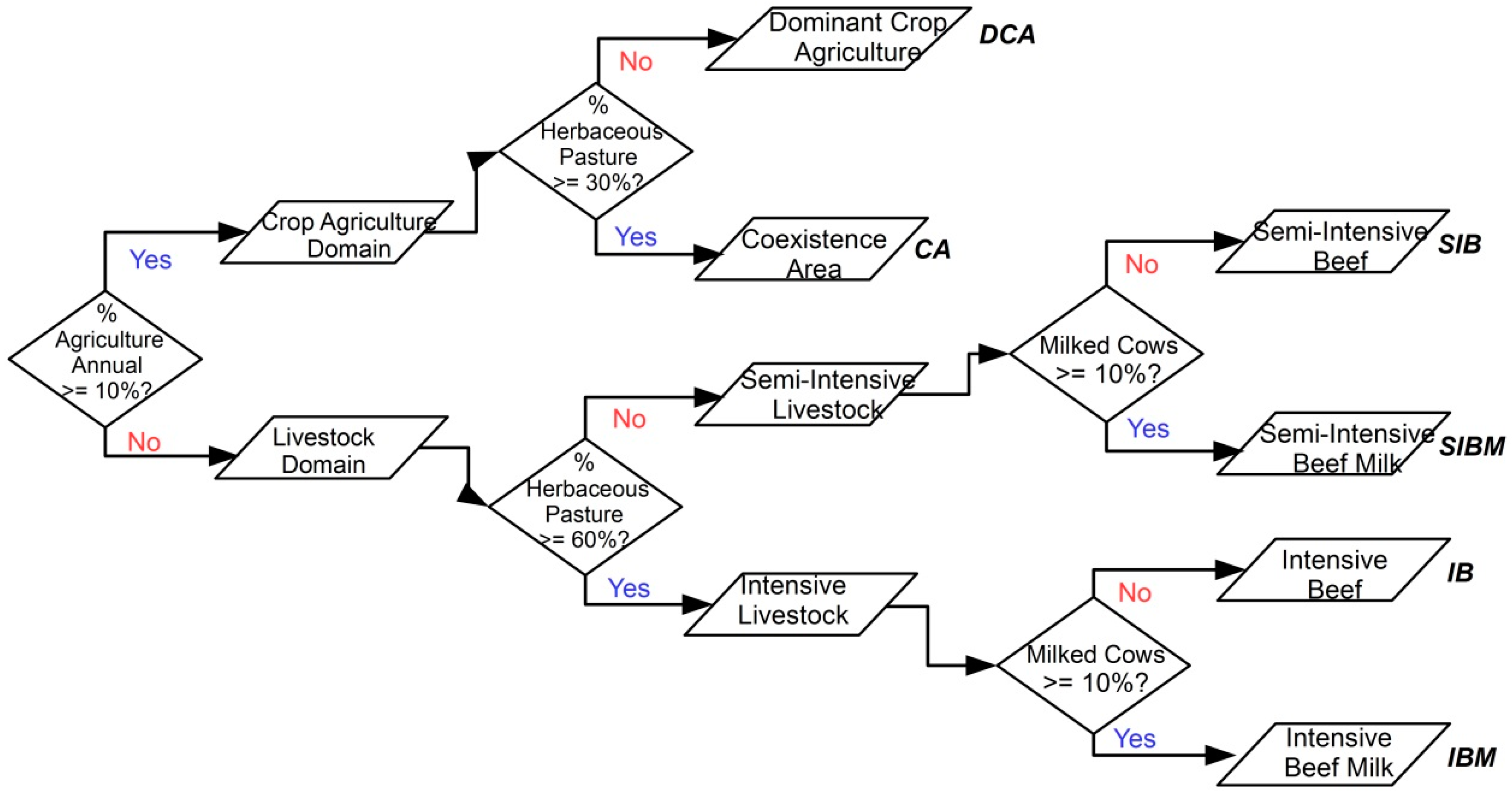
3.1. Identification of Agricultural Production Systems
3.2. Characterization of Agricultural Production Systems
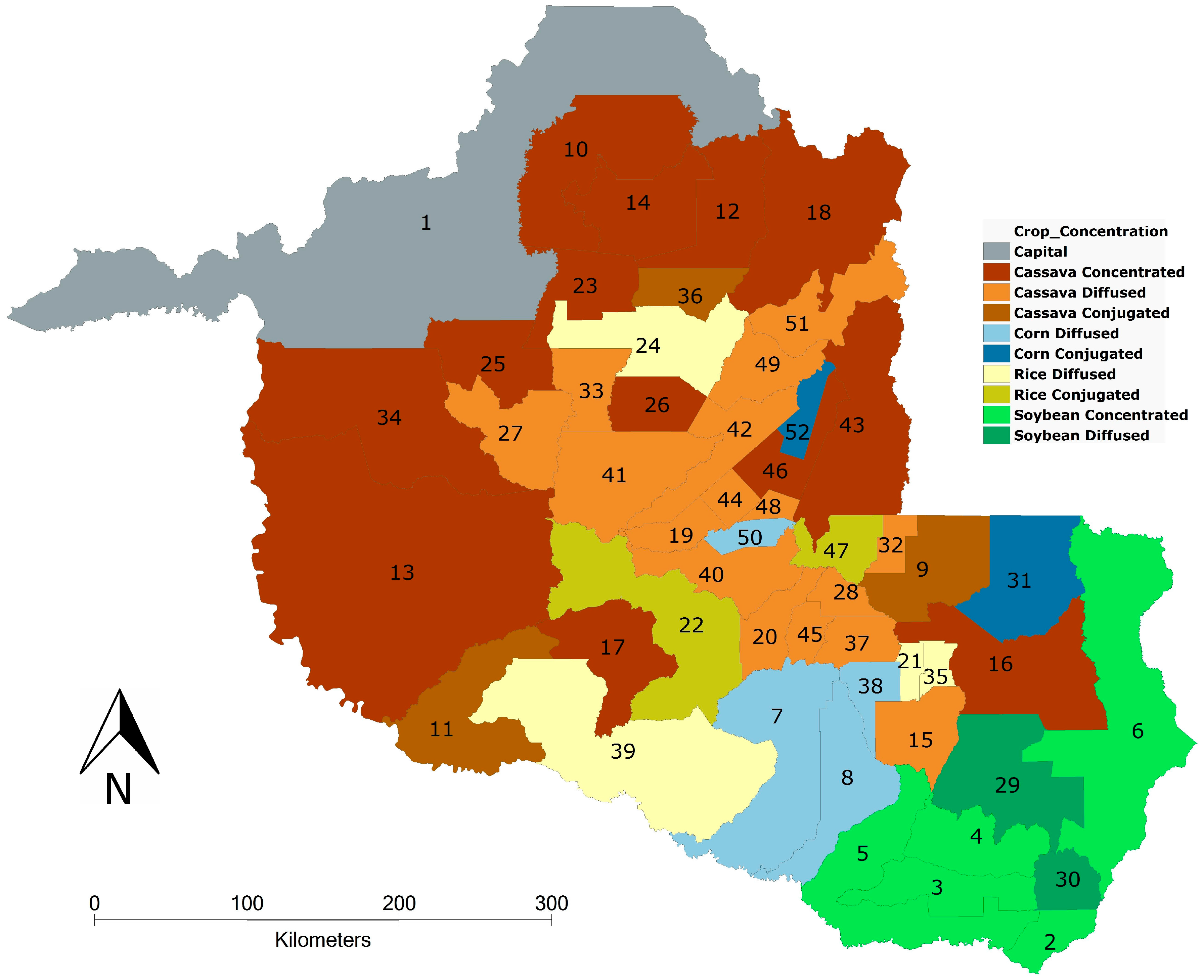
3.2.1. Concentration of Annual Crops and Coffee
3.2.2. Verification of Metrics
4. Results
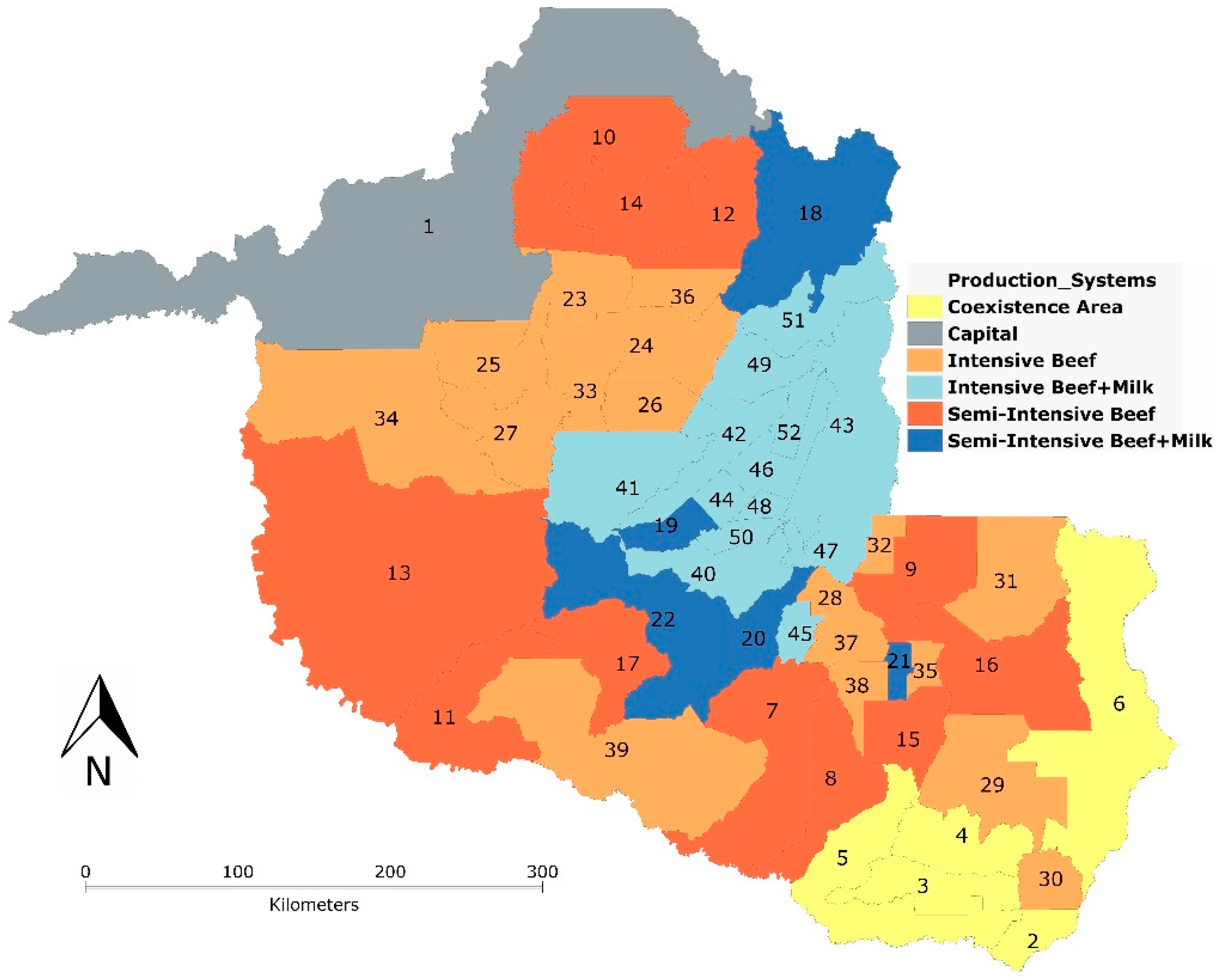
4.1. Localization of Agricultural Production Systems
4.2. Characterization of Agricultural Production Systems
4.2.1. Concentration of Annual Crops
4.2.2. Quantitative Analysis of Production Systems
5. Discussion
5.1. Agricultural Production
5.2. Economics
5.3. Territorial Configuration
5.4. Social Characteristics
6. Conclusions
Acknowledgments
Author Contributions
Conflicts of Interest
Abbreviations
| EMBRAPA | Brazilian Agricultural Research Corporation—Empresa Brasileira de Pesquisa Agropecuária (in Portuguese) |
| GDP | Gross Domestic Product—Produto Interno Bruto |
| IBGE | Brazilian Institute of Geography and Statistics—Instituto Brasileiro de Geografia e Estatística |
| INCRA | National Institute of Colonization and Agrarian ReformInstituto Nacional de Colonização e Reforma Agrária |
| INPE | Nacional Institute for Space research—Instituto Nacional de Pesquisas Espaciais |
| MHDI | Municipal Human Development Index—Indice de Desenvolvimento Humano Municipal (in portuguese) |
| PRODES | Project for the Monitoring of Brasilian Amazon Forest by satellite—Projeto de Monitoramento da Floresta Amazônica Brasileira por Satelite |
| SIPAM | Amazon Protection System—Sistema de proteção da Amazônia |
| TerraClass | Project for Monitoring the Land Use Land Cover in Brazilian Amazon—Projeto de Monitoramento do Uso e Cobertura da terra na Amazônica Brasileira |
Appendix A
Metrics

| Dimension | Metric | Description | Unit |
|---|---|---|---|
| agricultural production (Section 2.2.1) | AMProp | Mean area of properties within municipality (total area of properties/total number of properties) | km2 |
| NbovPast_T2 | Average capacity of TerraClass (Clean, dirty and regenerating) pastures = Total number of cattle in municipality 2010/Total number of TerraClass pastures in 2010 | Cattle/ha | |
| NVacReb_T2 | Proportion of milk cows within the total cattle population | % | |
| AMCafe_T2 | Mean cultivation area of coffee in the municipality in 2010 | ha | |
| DACafeT2 | Percent of deforested area in each municipality cultivated by coffee in 2010 | % | |
| economics (Section 2.2.2) PIB (Section 2.2.2.1) | PIB_T2 | Municipal GDP in 2010 | R$ × 1000 |
| PIBAgro_T2 | Municipal GDP for agricultural sector in 2010 | R$ × 1000 | |
| EvPIB_T1T2 | Evolution of GDP (2000 to 2010) = GDP 2010 – GDP 2000 | R$ × 1000 | |
| EvPIBAgro_T1T2 | Evolution of agricultural GDP (2000 to 2010) = agricultural GDP 2010 – agricultural GDP 2000 | R$ × 1000 | |
| PIBPRD_T2 | Relationship between GDP in 2010 and mean deforestation from PRODES in 2010 | R$ × 1000/km2 PRODES | |
| EvPIBPRD_T1T2 | Evolution of PIBPRD between 2000 and 2010 = PIBPRD_T2 – PIBPRD_T1 | R$ × 1000/km2 PRODES | |
| PIBAgroPRD_T2 | Relationship between agricultural GDP in 2010 de 2010 and mean deforestation from PRODES in 2010 | R$ × 1000/km2 PRODES | |
| EvPIBAgroPRD_T1T2 | Evolution of PIBAgroPRD between 2000 and 2010. = PIBAgroPRD_T2 – PIBAgroPRD_T1 | R$ × 1000/km2 PRODES | |
| PIBHab_T2 | Relationship between GDP 2010 and human population of municipality | R$ × 1000/hab. | |
| EvPIBHab_T1T2 | Evolution of the relationship between GDP and human population of municipality 2000–2010 | R$ × 1000/hab. | |
| PIBAgroPopR_T2 | Relationship between GDP and human population of the rural zone of the municipality in 2010 | R$ × 1000/hab. | |
| EvPIBAgroPopR_T1T2 | Evolution of the relationship between GDP and human population of the rural zone of the municipality 2000–2010 | R$ × 1000/hab. | |
| economics (Section 2.2.2) agricultural credit (Section 2.2.2.2) | NcrAg_2010 | Mean number of agricultural credit operations in municipality in 2010 | Unit |
| NTCrAg_T1T2 | Mean number of agricultural credit operations in municipality 2000–2010 | Unit | |
| RsMCrAg_T2 | Mean value of agricultural credit operations in municipality in 2010 | R$ × 1000 | |
| RsCrAgPRD_T2 | Relationship between total agricultural credit in 2010 and mean deforestation up to 2010 from PRODES | R$ × 1000/km2 Deforest. | |
| RsmCrAgPRD_T1T2 | Relationship between total agricultural credit in 2010 and mean deforestation between 2000 and 2010 from PRODES | R$ × 1000/km2 Deforet. | |
| economics (Section 2.2.2) Logística (Section 2.2.2.3) | DEst | Relationship between the total perimeter of roads and the total municipal area | km/km2 |
| DHdr | Total perimeter of polygons and vectors for hydrography of municipality/total area of municipality | km/km2 | |
| territorial configuration (Section 2.2.3) PRODES (Section 2.2.3.1) | AMPRD_T1T2 | Mean area of PRODES polygons 2000–2010 | km2 |
| APPRD_T1T2 | Area/Perimeter of PRODES polygons 2000–2010 | - | |
| DDesf_T2 | % deforestation in municipality from PRODES for 2010 | % | |
| DDesf_T1T2 | Evolution of % deforestation in municipality from PRODES between 2000 and 2010 = DdesfT2 – DdesfT1 | % | |
| TxMDesf_T1T2 | Mean rate of annual deforestation 2001–2010 from PRODES. | % | |
| territorial configuration (Section 2.2.3) TerraClass (Section 2.2.3.2) | AMPTC_T2 | Mean area of TerraClass 2010 polygons | km2 |
| APTC_T2 | Area/Perimeter of TerraClass 2010 polygons | - | |
| DPTC_T2 | Density of TerraClass 2010 polygons | poligons/km2 | |
| DATCAA_T2 | Density of annual crop class from TerraClass 2010 | % | |
| DATCMO_T2 | Density of mosaic occupation class from TerraClass 2010 | % | |
| DATCPL_T2 | Density of clean pasture class from TerraClass 2010 | % | |
| DATCPS_T2 | Density of dirty pasture class from TerraClass 2010 | % | |
| DATCRP_T2 | Density of regerating pasture class from TerraClass 2010 | % | |
| DATCVS_T2 | Density of secondary vegetation class from TerraClass 2010 | % | |
| territorial configuration (Section 2.2.3) Unidades Conservação Ambiental (Section 2.2.3.3) | DAUPA | % area of conservation units within municipality | % |
| Social characteristics (Section 2.2.4) | IDHM_T2 | Human development index (HDI) for 2010, composed of three dimensions of human development: longevity, education and income | Index (0 to 1) |
| IDHM_T1aT2 | Evolution of municipal HDI between 2000–2010 | Index (0 to 1) | |
| DPobre_T2 | % of adults with an income equal to or below R$14,000 per month in August 2010 | % of municipal population | |
| EvDPobre_T1T2 | Change in % of people living under poverty between 2000 and 2010 | % of municipal population | |
| DPAss | % municipal area occupied by settlement projects | % | |
| PopR_T2 | Population of the rural zone (demographic census 2010) | Unit | |
| EvPopR_T1T2 | Change in population in rural zone 2000–2010 | Unit | |
| PopRPRD_T2 | Relationship between population of the rural zone and mean deforestation to 2010 from PRODES | inhabitants /km2 Deforest. | |
| EvPopRPRD_T1T2 | Change in relationship between population of the rural zone and deforested from PRODES data, areas between 2000 and 2010 | inhabitants /km2 Deforest. | |
| EvPopRPRD_T1T2 (%) | % change in relationship between population of the rural zone in 2010 and mean deforestation from PRODES until 2010 | % |
| % Economic Contribution | ||||||||
|---|---|---|---|---|---|---|---|---|
| Municipality | Production System | Rice | Beans | Cassava | Corn | Soybean | Concentration | Principal Crop |
| Cabixi | CA | 4% | 0% | 4% | 13% | 79% | “concentrated” | Soybean |
| Cerejeiras | 11% | 0% | 2% | 20% | 67% | “concentrated” | Soybean | |
| Corumbiara | 12% | 0% | 3% | 11% | 74% | “concentrated” | Soybean | |
| Pimenteiras do Oeste | 7% | 0% | 1% | 2% | 90% | “concentrated” | Soybean | |
| Vilhena | 3% | 0% | 1% | 25% | 71% | “concentrated” | Soybean | |
| Rio Crespo | IB | 40% | 1% | 50% | 8% | 1% | “conjugated” | Cassava |
| Espigão D’Oeste | 14% | 1% | 42% | 43% | 0% | “conjugated” | Corn | |
| Alto Paraiso | 11% | 1% | 85% | 3% | 0% | “concentrated” | Cassava | |
| Buritis | 6% | 2% | 76% | 15% | 0% | “concentrated” | Cassava | |
| Cacaulândia | 1% | 0% | 96% | 4% | 0% | “concentrated” | Cassava | |
| Nova Mamoré | 1% | 1% | 91% | 7% | 0% | “concentrated” | Cassava | |
| Ariquemes | 44% | 2% | 26% | 18% | 10% | “diffused” | Rice | |
| Primavera de Rondônia | 48% | 1% | 33% | 18% | 0% | “diffused” | Rice | |
| São Francisco do Guaporé | 41% | 0% | 31% | 28% | 0% | “diffused” | Rice | |
| Campo Novo deRondônia | 26% | 3% | 42% | 29% | 0% | “diffused” | Cassava | |
| Castanheiras | 28% | 0% | 56% | 16% | 0% | “diffused” | Cassava | |
| Ministro Andreazza | 12% | 5% | 62% | 21% | 0% | “diffused” | Cassava | |
| Montenegro | 30% | 4% | 43% | 24% | 0% | “diffused” | Cassava | |
| Rolim de Moura | 19% | 7% | 53% | 21% | 0% | “diffused” | Cassava | |
| Santa Luzia D’Oeste | 21% | 15% | 29% | 35% | 0% | “diffused” | Corn | |
| Chupinguaia | 18% | 0% | 3% | 14% | 65% | “diffused” | Soybean | |
| Colorado do Oeste | 29% | 1% | 19% | 8% | 44% | “diffused” | Soybean | |
| Presidente Medici | IBM | 46% | 1% | 42% | 11% | 0% | “conjugated” | Rice |
| Vale do Paraiso | 6% | 3% | 24% | 67% | 0% | “conjugated” | Corn | |
| Ji-Paraná | 2% | 1% | 83% | 14% | 0% | “concentrated” | Cassava | |
| Ouro Preto do Oeste | 2% | 1% | 92% | 6% | 0% | “concentrated” | Cassava | |
| Alvorada D’Oeste | 38% | 3% | 39% | 19% | 0% | “diffused” | Cassava | |
| Gov.Jorge Teixeira | 8% | 24% | 45% | 23% | 0% | “diffused” | Cassava | |
| Jaru | 11% | 12% | 61% | 16% | 0% | “diffused” | Cassava | |
| Nova União | 12% | 13% | 56% | 18% | 0% | “diffused” | Cassava | |
| Novo Horizonte do Oeste | 34% | 6% | 38% | 22% | 0% | “diffused” | Cassava | |
| Teixeirópolis | 14% | 3% | 49% | 35% | 0% | “diffused” | Cassava | |
| Theobroma | 20% | 3% | 55% | 22% | 0% | “diffused” | Cassava | |
| Vale do Anari | 24% | 2% | 58% | 17% | 0% | “diffused” | Cassava | |
| Urupa | 9% | 10% | 39% | 42% | 0% | “diffused” | Corn | |
| Cacoal | SIB | 13% | 2% | 58% | 27% | 0% | “conjugated” | Cassava |
| Costa Marques | 24% | 2% | 66% | 8% | 0% | “conjugated” | Cassava | |
| Candeias do Jamari | 4% | 0% | 95% | 1% | 0% | “concentrated” | Cassava | |
| Cujubim | 14% | 5% | 77% | 5% | 0% | “concentrated” | Cassava | |
| Gujara-Mirim | 1% | 0% | 93% | 5% | 0% | “concentrated” | Cassava | |
| Itapuã do Oeste | 12% | 4% | 72% | 3% | 9% | “concentrated” | Cassava | |
| Pimenta Bueno | 10% | 0% | 80% | 9% | 0% | “concentrated” | Cassava | |
| Seringueiras | 15% | 1% | 74% | 9% | 0% | “concentrated” | Cassava | |
| Parecis | 14% | 3% | 46% | 37% | 0% | “diffused” | Cassava | |
| Alta Floresta do Oeste | 7% | 27% | 20% | 46% | 0% | “diffused” | Corn | |
| Alto Alegre do Parecis | 10% | 24% | 26% | 40% | 0% | “diffused” | Corn | |
| São Miguel do Guaporé | SIBM | 44% | 1% | 43% | 11% | 0% | “conjugated” | Rice |
| Machadinho D’Oeste | 10% | 3% | 76% | 12% | 0% | “concentrated” | Cassava | |
| São Felipe D’Oeste | 41% | 13% | 8% | 38% | 0% | “diffused” | Rice | |
| Mirante da Serra | 15% | 8% | 51% | 26% | 0% | “diffused” | Cassava | |
| Nova Brasilândia D’Oeste | 18% | 5% | 62% | 16% | 0% | “diffused” | Cassava | |
References
- Droulers, M. L’Amazonie Vers un Développement Durable, 1st ed.; Armand Colin: Paris, France, 2004. [Google Scholar]
- Becker, B.K. Amazônia: Geopolítica na Virada do III Milênio; Editora Garamond: Rio de Janeiro, Brazil, 2004. [Google Scholar]
- Becker, B.K. A Amazônia e a política ambiental brasileira. Geografia 2004, 6, 7–20. [Google Scholar]
- Aguiar, A.P.D.; Câmara, G.; Escada, M.I.S. Spatial statistical analysis of land-use determinants in the Brazilian Amazonia: Exploring intra-regional heterogeneity. Ecol. Model. 2007, 209, 169–188. [Google Scholar] [CrossRef]
- Richards, P.D.; Walker, R.T.; Arima, E.Y. Spatially complex land change: The Indirect effect of Brazil’s agricultural sector on land use in Amazonia. Glob. Environ. Chang. 2014, 29, 1–9. [Google Scholar] [CrossRef] [PubMed]
- Brondizio, E.S.; Moran, E.F. Human dimensions of climate change: The vulnerability of small farmers in the Amazon. Philos. Trans. R. Soc. Lond. B Biol. Sci. 2008, 363, 1803–1809. [Google Scholar] [CrossRef] [PubMed]
- Browder, J.O.; Pedlowski, M.A.; Walker, R.; Wynne, R.H.; Summers, P.M.; Abad, A.; Becerra-Cordoba, N.; Mil-Homens, J. Revisiting theories of frontier expansion in the Brazilian amazon: A survey of the colonist farming population in Rondônia’s post-frontier, 1992–2002. World Dev. 2008, 36, 1469–1492. [Google Scholar] [CrossRef]
- De Assis Costal, F. Mercado e produção de terras na Amazônia: Avaliação referida a trajetórias tecnológicas. Bol. Mus. Para. Emilio Goeldi Ciênc. Hum. 2010, 5, 25–39. [Google Scholar]
- Santos Junior, R.A.O.; Costa, F.D.A.; Aguiar, A.P.D.; de Toledo, P.M.; Vieira, I.C.G.; Câmara, G. Desmatamento, trajetórias tecnológicas e metas de contenção de emissões na Amazônia. Cienc. Cult. 2010, 62, 56–59. [Google Scholar]
- De Mello, N.A.; Théry, H. L’État brésilien et l’environnement en Amazonie: Évolutions, contradictions et conflits. L’esp. Géogr. 2003, 32, 3–20. [Google Scholar]
- Perz, S.G. The effects of household asset endowments on agricultural diversity among frontier colonists in the Amazon. Agrofor. Syst. 2005, 63, 263–279. [Google Scholar] [CrossRef]
- Williams, K.J.H.; Schirmer, J. Understanding the relationship between social change and its impacts: The experience of rural land use change in south-eastern Australia. J. Rural Stud. 2012, 28, 538–548. [Google Scholar] [CrossRef]
- Woods, M. Rural geography III: Rural futures and the future of rural geography. Prog. Hum. Geogr. 2012, 36, 125–134. [Google Scholar] [CrossRef]
- Li, Y.; Long, H.; Liu, Y. Spatio-temporal pattern of China’s rural development: A rurality index perspective. J. Rural Stud. 2015, 38, 12–26. [Google Scholar] [CrossRef]
- Anselin, L.; Sridharan, S.; Gholston, S. Using exploratory spatial data analysis to leverage social indicator databases: The discovery of interesting patterns. Soc. Indic. Res. 2007, 82, 287–309. [Google Scholar] [CrossRef]
- Grigg, D. An introduction to Agricultural Geography, 2nd ed.; Routledge: London, UK, 2003. [Google Scholar]
- Pacione, M. Progress in Agricultural Geography, 1st ed.; Routledge: New York, NY, USA, 2013. [Google Scholar]
- Pecqueur, B. Esquisse d’ une géographie économique territoriale. L’Espace. Géogr. 2014, 43, 198–214. [Google Scholar]
- De Souza, E.C.; da Silva, G.J.C. Dinâmica espacial e formação de clusters significativos no setor agropecuário de Minas Gerais. Rev. Econ. Tecnol. 2012, 6, 107–116. [Google Scholar] [CrossRef]
- Soler, L.S.; Verburg, P.H. Combining remote sensing and household level data for regional scale analysis of land cover change in the Brazilian Amazon. Reg. Environ. Chang. 2010, 10, 371–386. [Google Scholar] [CrossRef] [Green Version]
- Espindola, G.M.; de Aguiar, A.P.D.; Pebesma, E.; Câmara, G.; Fonseca, L. Agricultural land use dynamics in the Brazilian Amazon based on remote sensing and census data. Appl. Geogr. 2012, 32, 240–252. [Google Scholar] [CrossRef]
- Helfand, S.M.; Moreira, A.R.B.; Figueiredo, A.M.R. Explicando as diferenças de pobreza entre produtores agrícolas no Brasil: Simulações contrafactuais com o censo agropecuário 1995–1996. Rev. Econ. Sociol. Rural 2011, 49, 391–418. [Google Scholar] [CrossRef]
- Southworth, J.; Munroe, D.; Nagendra, H. Land cover change and landscape fragmentation—Comparing the utility of continuous and discrete analyses for a western Honduras region. Agric. Ecosyst. Environ. 2004, 101, 185–205. [Google Scholar] [CrossRef]
- Becker, B.K. Amazônia; Editora Ática: São Paulo, Brazil, 1990. [Google Scholar]
- Théry, H. Routes et déboisement en Amazonie brésilienne, Rondônia 1974–1996. Mappemonde 1997, 97, 35–40. [Google Scholar]
- Théry, H. Rondônia, Mutations d’un Territoire Fédéral en Amazonie Brésilienne; Université Panthéon-Sorbonne—Paris I: Paris, France, 1976. [Google Scholar]
- Coy, M. Desenvolvimento regional na periferia amazônica: Organização do espaço, conflitos de interesses e programas de planejamento dentro de uma região de ‘fronteira’: O caso de Rondônia. In Fronteiras; Editora Universidade de Brasília: Brasilia, Brazil, 1988; pp. 167–194. [Google Scholar]
- Théry, H. Situações da Amazônia no Brasil e no continente. Estud. Av. 2005, 19, 37–49. [Google Scholar] [CrossRef]
- Xavier, A.D.S. Fronts Pionniers D’amazonie, Les Dinamiques Paysannes au Brésil, 1st ed.; CNRS Editions: Paris, France, 2006. [Google Scholar]
- Fiori, M.F.; Fiori, L.E.; Nenevé, M. Colonização agrícola de Rondônia e (não) obrigatoriedade de desmatamento como garantia de posse sobre a propriedade rural. Novos Cad. Naea 2013, 16, 9–22. [Google Scholar] [CrossRef]
- Instituto Nacional de Pesquisas Espaciais (INPE). Projeto PRODES—Monitoramento da Floresta Amazônica Brasileira por Satélite. 2015. Available online: http://www.dpi.inpe.br/prodesdigital/prodesmunicipal.php (accessed on 12 August 2015).
- Da Coata Silva, R.G. A regionalização do agronegócio da soja em Rondônia. GEOUSP Espaç. Tempo (Online) 2014, 18, 298–312. [Google Scholar] [CrossRef]
- De Almeida, C.A.; Coutinho, A.C.; Esquerdo, J.C.D.M.; Adami, M.; Venturieri, A.; Diniz, C.G.; Dessay, N.; Durieux, L.; Gomes, A.R. High spatial resolution land use and land cover mapping of the 1 Brazilian Legal Amazon in 2008 using Landsat-5/TM and MODIS data. Acta Amaz. 2016, 46, 291–302. [Google Scholar]
- Instituto Brasileiro de Geografia e Estatística (IBGE). IBGE Cidades@. 2012. Available online: http://www.cidades.ibge.gov.br/xtras/home.php (accessed on 27 May 2012). [Google Scholar]
- Tsunechiro, A.; Coelho, P.J.; Miura, M. Valor da produção agropecuária no Brasil, por unidade da federação em 2008. Rev. Inf. Econ. 2010, 40, 62–79. [Google Scholar]
- Bacen. Anuário Estatístico do Crédito Rural. 2015. Available online: http://www.bcb.gov.br/?RELRURAL (accessed on 19 February 2015). [Google Scholar]
- Sistema de Proteção da Amazônia (SIPAM). Malha Viária Geral do Estado de Rondônia. 2010. Available online: http://www.metadados.inde.gov.br/geonetwork/srv/por/metadata.show?id=17627&currTab=simple (accessed on 23 February 2015). [Google Scholar]
- Naveh, Z. From biodiversity to ecodiversity: A landscape-ecology approach to conservation and restoration. Restor. Ecol. 1994, 2, 180–189. [Google Scholar] [CrossRef]
- Wiens, J.A. What is landscape ecology, really? Landsc. Ecol. 1992, 7, 149–150. [Google Scholar] [CrossRef]
- Cruz, C.; Madureira, H.; Marques, J. Análise espacial e estudo da fragmentação da Paisagem da Aboboreira. Rev. Geogr. Ordenam. Territ. 2013, 1, 57–82. [Google Scholar] [CrossRef]
- Carrão, H.M.S.; Caetano, M.; Neves, N. LANDIC—Cálculo de indicadores de paisagem em ambiente SIG. In Proceedings of Encontro de Utilizadores de Informação Geográfica—ESIG 2001, Oeiras, Portugal, 28–30 November 2001.
- Pereira, J.L.G.; Batista, G.T.; Thalês, M.C.; Roberts, D.A.; Venturieri, A. Métricas da paisagem na caracterização da evolução da ocupação da Amazônia. Geografia 2001, 26, 59–90. [Google Scholar]
- Johan, O.; Xavier, A.D.S.; Thibaud, D.; Valery, G.; Michel, G.; Antoine, L.; Rennes, U.; Moal, L.; Letg, U.M.R.; Cnrs, U.M.R.; et al. Utilisation de la télédétection et de donnés socio-économiques et écologiques pour compreendre l’impact des dynamiques de l’occupation des sols a Pacajà (Brésil). Rev. Fr. Photogramm. Télédétec. 2012, 198–199, 8–24. [Google Scholar]
- Ziolkowski, D.; Turlej, K.; Bochenek, Z. Indicators of landscape diversity derived from remote sensing based land cover maps—Spatial and thematic aspects. Ecol. Quest. 2013, 17, 113–129. [Google Scholar] [CrossRef]
- Gustafson, E. Quantifying landscape spatial pattern: What is the state of the art? Ecosystems 1998, 1, 143–156. [Google Scholar] [CrossRef]
- Ministério do Meio Ambiente. Cadastro Nacional de Unidade de Conservação. 2015. Available online: http://www.mma.gov.br/areas-protegidas/cadastro-nacional-de-ucs/dados-georreferenciados (accessed on 18 May 2016). [Google Scholar]
- Ceron, A.O.; de Oliveira Girardi, L.H. Geografia agrária e metodologia de pesquisa/agrarian geography and research metodology. CAMPO-TERRITÓRIO Rev. Geogr. Agrár. 2007, 2, 4–16. [Google Scholar]
- Coelho, V.H.R.; Montenegro, S.M.G.L.; de Almeida, C.N.; de Lima, E.R.V.; Neto, A.R.; de Moura, G.S.S. Dinâmica do uso e ocupação do solo em uma bacia hidrográfica do semiárido brasileiro. R. Bras. Eng. Agríc. Ambient. 2014, 18, 64–72. [Google Scholar] [CrossRef]
- Siedenberg, D.R. Indicadores de desenvolvimento socioeconomico. Desenvolv. Quest. 2003, 1, 45–71. [Google Scholar]
- Jannuzzi, P.D.M. Considerações sobre o uso, mau uso e abuso dos indicadores sociais na formulação e avaliação de políticas públicas municipais. Rev. Adm. Pública 2002, 36, 51–72. [Google Scholar]
- Programa das Nações Unidas para o Desenvolvimento (PNUD); Instituto de Pesquisa Econômica Aplicada (IPEA); Fundação João Pinheiro. O Atlas do Desenvolvimento Humano no Brasil. 2015. Available online: http://www.atlasbrasil.org.br/2013/pt/o_atlas/o_atlas_/ (accessed on 19 February 2015).
- Instituto Nacional de Colonização e Reforma Agrária (INCRA). Acervo Fundiário. In Acervo Fundiário I3Geo; 2015. Available online: http://acervofundiario.incra.gov.br/i3geo/interface/incra.html?63t9hg62kbk1eulgspj2ue5ui6 (accessed on 23 February 2015). [Google Scholar]
- Ligêza, A. Logical foundations for rule-based systems. In Logical Foundations for Rule-Based Systems; Springer: Berlin/Heidelberg, Germany, 2006; pp. 191–198. [Google Scholar]
- Geist, H.J.; Lambin, E.F. What Drives Tropical Deforestation? LUCC Report Series, No 4; LUCC International Project Office: Louvain-la-Neuve, Belgium, 2001. [Google Scholar]
- Margulis, S. Causes of Deforestation of the Brazilian Amazon; The World Bank: Washington, DC, USA, 2003. [Google Scholar]
- Godar, J.; Gardner, T.A.; Tizado, E.J.; Pacheco, P. Actor-specific contributions to the deforestation slowdown in the Brazilian Amazon. Proc. Natl. Acad. Sci. USA 2014, 111, 15591–15596. [Google Scholar] [CrossRef] [PubMed]
- Chomitz, K.M.; Thomas, T.S. Geographic Patterns of Land Use and Land Intensity in the Brazilian Amazon; World Bank Policy Research Working Paper No. 2687; The World Bank: New York, NY, USA, 2001. [Google Scholar]
- Agência de Defesa Sanitária Agrosilvopastoril do Estado de Rondônia (IDARON). Levantamento de Dados Sobre a Produção de Leite em Rondônia. 2013. Available online: http://www.idaron.ro.gov.br/Multimidia/downloads/docs/Producao_de_leite_em_Rondonia-divulgacao.pdf (accessed on 19 February 2015). [Google Scholar]
- Soler, L.D.S.; Verburg, P.H.; Alves, D. Evolution of land use in the Brazilian Amazon: From frontier expansion to market chain dynamics. Land 2014, 3, 981–1014. [Google Scholar] [CrossRef]
- Da Costa Silva, R.G. Amazônia globalizada: Da fronteira agrícola ao território do agronegócio—O exemplo de Rondônia. Confins 2015, 23. [Google Scholar] [CrossRef]
- Hurtienne, T.P. Agricultura familiar e desenvolvimento rural sustentável na Amazônia. Novos Cad. Naea 2005, 8, 19–71. [Google Scholar] [CrossRef]
- Becker, B.K. Reflexões sobre a Geopolítica e a logística da soja na Amazônia. In Dimensões Humanas da Biosfera-Atmosfera na Amazônia; Edusp: São Paulo, Brazil, 2007; p. 176. [Google Scholar]
- Simon, M.F.; Garagorry, F.L. The expansion of agriculture in the Brazilian Amazon. Environ. Conserv. 2006, 32, 203–212. [Google Scholar] [CrossRef]
- Euclides, V.P.B. Produção intensiva de carne bovina em pasto. Simp. Prod. Gado Corte 2001, 2, 55–82. [Google Scholar]
- Oliveira, R.L.; de Freitas Barbosa, M.A.A.; Ladeira, M.M.; da Silva, M.M.P.; Ziviani, A.C.; Bagaldo, A.R. Nutrição e manejo de bovinos de corte na fase de cria. Rev. Bras. Saúde Prod. Anim. 2006, 7, 57–86. [Google Scholar]
- Instituto Brasileiro de Geografia e Estatísitca (IBGE). Série Relatórios Metodológicos. Produto Interno Bruto dos Municípios; IBGE: Rio de Janeiro, Brazil, 2004.
- Bonelli, R. Impactos Econômicos e Sociais de Longo Prazo da Expansão Agropecuária no Brasil: Revolução Invisível e Inclusão Social; Instituto de Pesquisa Econômica Aplicada: Rio de Janeiro, Brazil, 2001.
- De Janvry, A.; Sadoulet, E. Agricultural growth and poverty reduction: Additional evidence. World Bank Res. Obs. 2010, 25, 1–20. [Google Scholar] [CrossRef]
- Le Tourneau, F. La distribution du peuplement en Amazonie brésilienne : L’apport des données par secteur de recensement contexte pionnier de l’Amazonie brésilienne, et nous proposions quelques La représentation de la population en Amazonie et ses enjeux. L’esp. Géogr. 2009, 38, 359–375. [Google Scholar]
- Alves, D.S.; Escada, M.I.S.; Pereira, J.L.G.; de Albuquerque Linhares, C. Land use intensification and abandonment in Rondônia, Brazilian Amazônia. Int. J. Remote Sens. 2003, 24, 899–903. [Google Scholar] [CrossRef]
- Soler, L.D.S.; Escada, M.I.S.; Verburg, P.H. Quantifying deforestation and secondary forest determinants for different spatial extents in an Amazonian colonization frontier (Rondonia). Appl. Geogr. 2009, 29, 182–193. [Google Scholar] [CrossRef]
- Vale, P.M.; Andrade, D.C. Comer carne salva a Amazônia? A produtividade da pecuária em Rondônia e sua relação com o desmatamento. Estud. Soc. Agric. 2012, 20, 381–408. [Google Scholar]
- Bermann, C. Impasses e controvérsias da hidreletricidade. Estud. Av. 2007, 21, 139–153. [Google Scholar] [CrossRef]
- Tilt, B.; Braun, Y.; He, D. Social impacts of large dam projects: A comparison of international case studies and implications for best practice. J. Environ. Manag. 2009, 90, S249–S257. [Google Scholar] [CrossRef] [PubMed]
- Browder, J.O.; Pedlowski, M.A.; Summers, P.M. Land use patterns in the Brazilian Amazon: Comparative farm-level evidence from Rondônia. Hum. Ecol. 2004, 32, 197–224. [Google Scholar] [CrossRef]


| Rules | Class of Concentration | Number of Principal Crops |
|---|---|---|
| C1 ≥ 67% | “concentrated” | one crop |
| C1 < 67% and C1 + C2 ≥ 84% | “conjugated” | two crops |
| C1 + C2 < 84% | “diffused” | three or more crops |
| Production System | Concentration | Principal Crop | Municipality |
|---|---|---|---|
| CA | “concentrated” | Soybean | Cabixi (2), Cerejeiras (3), Corumbiara (4), Pimenteiras do Oeste (5), Vilhena (6) |
| IB | “conjugated” | Cassava | Rio Crespo (36) |
| Corn | Espigão D’Oeste (31) | ||
| “concentrated” | Cassava | Alto Paraiso (23), Buritis (25), Cacaulândia (26), Nova Mamoré (34) | |
| “diffused” | Rice | Ariquemes (24), Primavera de Rondônia (35), São Francisco do Guaporé (39) | |
| Cassava | Campo Novo de Rondônia (27), Castanheiras (28), Ministro Andreazza (32), Montenegro (33), Rolim de Moura (37) | ||
| Corn | Santa Luzia D’Oeste (38) | ||
| Soybean | Chupinguaia (29), Colorado do Oeste (30) | ||
| IBM | “conjugated” | Rice | Presidente Medici (47) |
| Corn | Vale do Paraiso (52) | ||
| “concentrated” | Cassava | Ji-Paraná (43), Ouro Preto do Oeste (46) | |
| “diffused” | Cassava | Alvorada D’Oeste (40), Gov.Jorge Teixeira (41), Jaru (42), Nova União (44), Novo Horizonte do Oeste (45), Teixeirópolis (48), Theobroma (49), Vale do Anari (51) | |
| Corn | Urupa (50) | ||
| SIB | “conjugated” | Cassava | Cacoal (9), Costa Marques (11) |
| “concentrated” | Cassava | Candeias do Jamari (10), Cujubim (12), Guajara-Mirim (13), Itapuã do Oeste (14), Pimenta Bueno (16), Seringueiras (17) | |
| “diffused” | Cassava | Parecis (15) | |
| Corn | Alta Floresta do Oeste (7), Alto Alegre do Parecis (8) | ||
| SIBM | “conjugated” | Rice | São Miguel do Guaporé (22) |
| “concentrated” | Cassava | Machadinho D’Oeste (18) | |
| “diffused” | Rice | São Felipe D’Oeste (21) | |
| Cassava | Mirante da Serra (19), Nova Brasilândia D’Oeste (20) |
| Agricultural Production System | ||||||
|---|---|---|---|---|---|---|
| Dimension | Metric | CA | IB | IBM | SIB | SIBM |
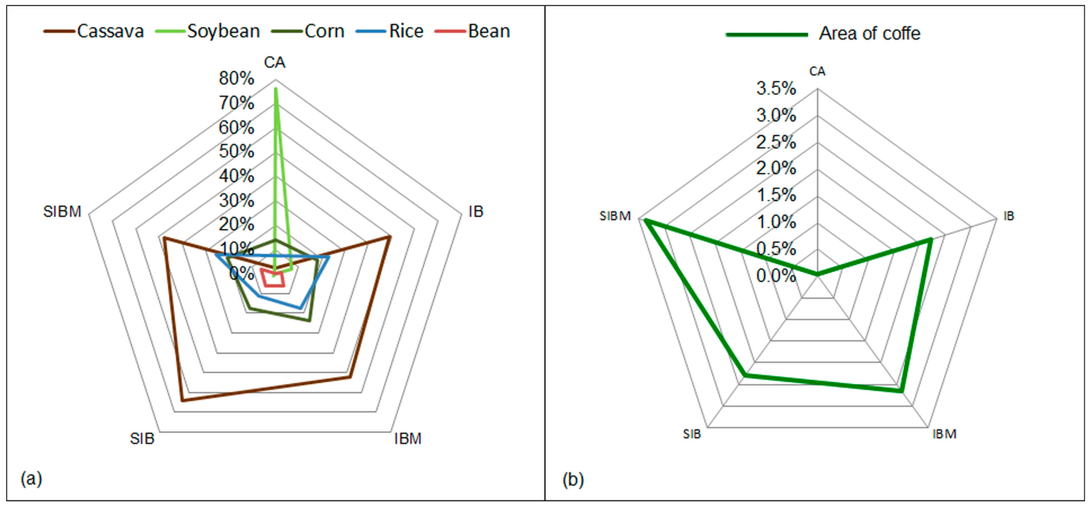
| agricultural production (Section 2.2.1) | AMProp | 2.65 (a) | 1.24 (b) | 0.69 (b) | 1.45 (ab) | 0.59 (b) |
| NbovPast_T2 | 1.74 (ab) | 2.05 (ab) | 2.21 (a) | 1.62 (b) | 1.91 (ab) | |
| NvacReb_T2 | 5.49 (c) | 5.93 (c) | 19.67 (a) | 4.87 (c) | 15.18 (b) | |
| AMCafe_T2 | 50 (c) | 2487 (bc) | 3043 (abc) | 3346 (ab) | 7376 (a) | |
| DACafe_T2 | 0.04 | 0.11 | 2.21 | 2.66 | 2.27 | |
| economics (Section 2.2.2) PIB (Section 2.2.2.1) | PIB_T2 | 414,322.20 | 343,418.94 | 329,017.15 | 267,644.00 | 196,971.80 |
| PIBAgro_T2 | 98,103.80 | 87,592.06 | 72,330.62 | 80,524.00 | 75,123.80 | |
| EvPIB_T1T2 | 292,951.80 | 246,097.56 | 222,601.00 | 211,807.58 | 145,211.20 | |
| EvPIBAgro_T1T2 | 72,661.80 | 67,386.13 | 49,017.15 | 68,555.92 | 59,915.20 | |
| PIBPRD_T2 | 286.55 | 184.94 | 195.06 | 160.52 | 201.73 | |
| EvPIBPRD_T1T2 | 181.39 | 121.63 | 125.18 | 111.32 | 142.16 | |
| PIBAgroPRD_T2 | 73.90 | 53.54 | 56.13 | 47.08 | 81.36 | |
| EvPIBAgroPRD_T1T2 | 49.86 | 37.67 | 36.25 | 36.33 | 64.37 | |
| PIBHab_T2 | 22.21 (a) | 15.04 (ab) | 12.26 (b) | 13.95 (ab) | 14.68 (ab) | |
| EvPIBHab_T1T2 | 16.71 | 10.95 | 8.61 | 10.26 | 11.27 | |
| PIBAgroPopR_T2 | 34.54 (a) | 12.66 (b) | 8.44 (b) | 13.64 (b) | 9.56 (b) | |
| EvPIBAgroPopR_T1T2 | 26.51 (a) | 10.09 (b) | 6.45 (b) | 11.56 (b) | 8.09 (b) | |
| economics (Section 2.2.2) agricultural credit (Section 2.2.2.2) | NcrAg_T2 | 397.80 | 453.65 | 474.00 | 458.00 | 667.20 |
| NTCrAg_T1T2 | 4522.00 | 4582.00 | 6675.92 | 5673.55 | 8361.40 | |
| RsMCrAg_T2 | 56.13 (a) | 30.79 (ab) | 29.45 (ab) | 31.23 (ab) | 12.56 (b) | |
| RsCrAgPRD_T2 | 15.35 (a) | 7.38 (b) | 10.23 (ab) | 6.19 (b) | 8.36 (a) | |
| RsMCrAgPRD_T1T2 | 8.95 (ab) | 4.11 (ab) | 4.58 (ab) | 3.10 (b) | 10.05 (a) | |
| economics (Section 2.2.2) logístics (Section 2.2.2.3) | DEst | 7.95 | 6.97 | 6.76 | 15.36 | 8.59 |
| DHdr | 0.058 | 0.047 | 0.061 | 0.062 | 0.066 | |
| territorial configuration (Section 2.2.3) PRODES (Section 2.2.3.1) | AMPRD_T1T2 (km2) | 0.220 (a) | 0.183 (b) | 0.140 (c) | 0.179 (b) | 0.150 (c) |
| APPRD_T1T2 | 62.02 (a) | 60.36 (b) | 52.81 (e) | 59.41 (c) | 55.94 (d) | |
| DDesf_T2 (%) | 41.5 (b) | 66.7 (a) | 71.4 (a) | 32.4 (b) | 54.4 (ab) | |
| DDesf_T1T2 (%) | 4.9 | 10.4 | 6.3 | 11.6 | 8.3 | |
| TxMDesf_T1aT2 (%) | 1.4 (b) | 3.0 (a) | 3.4 (a) | 2.0 (ab) | 2.3 (ab) | |
| territorial configuration (Section 2.2.3) TerraClass (Section 2.2.3.2) | AMPTC_T2 (km2) | 0.712 | 0.651 | 0.413 | 0.418 | 0.360 |
| APTC_T2 | 44.67 (a) | 42.53 (c) | 38.26 (e) | 43.42 (b) | 40.94 (d) | |
| DPTC_T2 | 1.94 (b) | 3.17 (ab) | 3.40 (a) | 2.07 (ab) | 3.18 (ab) | |
| DATCAA_T2 | 24.12 (a) | 1.19 (b) | 0.07 (b) | 0.72 (b) | 0.52 (b) | |
| DATCMO_T2 | 0.22 (b) | 1.43 (b) | 2.33 (ab) | 1.58 (b) | 6.23 (a) | |
| DATCPL_T2 | 45.07 (c) | 68.79 (a) | 73.52 (a) | 52.90 (bc) | 56.10 (b) | |
| DATCPS_T2 | 6.07 (b) | 7.16 (b) | 5.55 (b) | 13.32 (a) | 11.42(ab) | |
| DATCRP_T2 | 8.47 (a) | 3.01 (b) | 2.25 (b) | 9.01 (a) | 7.30 (a) | |
| DATCVS_T2 | 13.90 | 16.37 | 15.79 | 19.44 | 17.72 | |
| territorial configuration (Section 2.2.3) conservation units (Section 2.2.3.3) | DAUPA (%) | 29.1 (ab) | 12.2 (b) | 16.5 (b) | 43.9 (a) | 27.9 (ab) |
| social characteristics (Section 2.2.4) | IDHM_T2 | 0.67 | 0.65 | 0.64 | 0.63 | 0.64 |
| IDHM_T1aT2 | 0.16 | 0.17 | 0.18 | 0.16 | 0.18 | |
| DPobre_T2 | 16.76 | 19.87 | 23.33 | 23.13 | 26.52 | |
| EvDPobre_T1T2 | −17.85 | −15.89 | −15.83 | −16.45 | −13.32 | |
| DPAss | 0.20 | 0.47 | 0.52 | 0.20 | 0.28 | |
| PopR_T2 | 3486.00 (b) | 7387.81 (ab) | 8449.85 (ab) | 6695.25 (ab) | 9964.40 (a) | |
| EvPopR_T1T2 | −657.80 | −1141.31 | −2959.54 | 408.42 | −684.60 | |
| PopRPRD_T2 | 2.62 (c) | 4.81 (b) | 6.97 (a) | 4.24 (b) | 8.08 (a) | |
| EvPopRPRD_T1T2 | −0.99 (a) | −2.05 (ab) | −3.36 (bc) | −1.83 (a) | −3.59 (c) | |
| EvPopRPRD_T1T2 (%) | −24.31 | −27.37 | −32.48 | −26.07 | −29.06 | |
© 2016 by the authors; licensee MDPI, Basel, Switzerland. This article is an open access article distributed under the terms and conditions of the Creative Commons Attribution (CC-BY) license (http://creativecommons.org/licenses/by/4.0/).
Share and Cite
Almeida, C.; Mourão, M.; Dessay, N.; Lacques, A.-E.; Monteiro, A.; Durieux, L.; Venturieri, A.; Seyler, F. Typologies and Spatialization of Agricultural Production Systems in Rondônia, Brazil: Linking Land Use, Socioeconomics and Territorial Configuration. Land 2016, 5, 18. https://doi.org/10.3390/land5020018
Almeida C, Mourão M, Dessay N, Lacques A-E, Monteiro A, Durieux L, Venturieri A, Seyler F. Typologies and Spatialization of Agricultural Production Systems in Rondônia, Brazil: Linking Land Use, Socioeconomics and Territorial Configuration. Land. 2016; 5(2):18. https://doi.org/10.3390/land5020018
Chicago/Turabian StyleAlmeida, Cláudio, Moisés Mourão, Nadine Dessay, Anne-Elisabeth Lacques, Antônio Monteiro, Laurent Durieux, Adriano Venturieri, and Frédérique Seyler. 2016. "Typologies and Spatialization of Agricultural Production Systems in Rondônia, Brazil: Linking Land Use, Socioeconomics and Territorial Configuration" Land 5, no. 2: 18. https://doi.org/10.3390/land5020018