
Modeling the Impact of Land Use Optimization on Non-Point Source Pollution: Evidence from Chinese Reservoir Watershed

Abstract
:1. Introduction
- (a)
- Evaluating the role of the coupled model in optimizing land use and monitoring NPS pollution within the watershed;
- (b)
- Contrasting NPS pollution loads pre- and post-land use optimization, conducting an analysis on the impact of land use changes and optimization strategies on NPS pollution distribution and magnitude.
- (c)
- Assessing the effectiveness of the proposed coupled multi-model approach for controlling non-point source pollution.
2. Materials and Methods
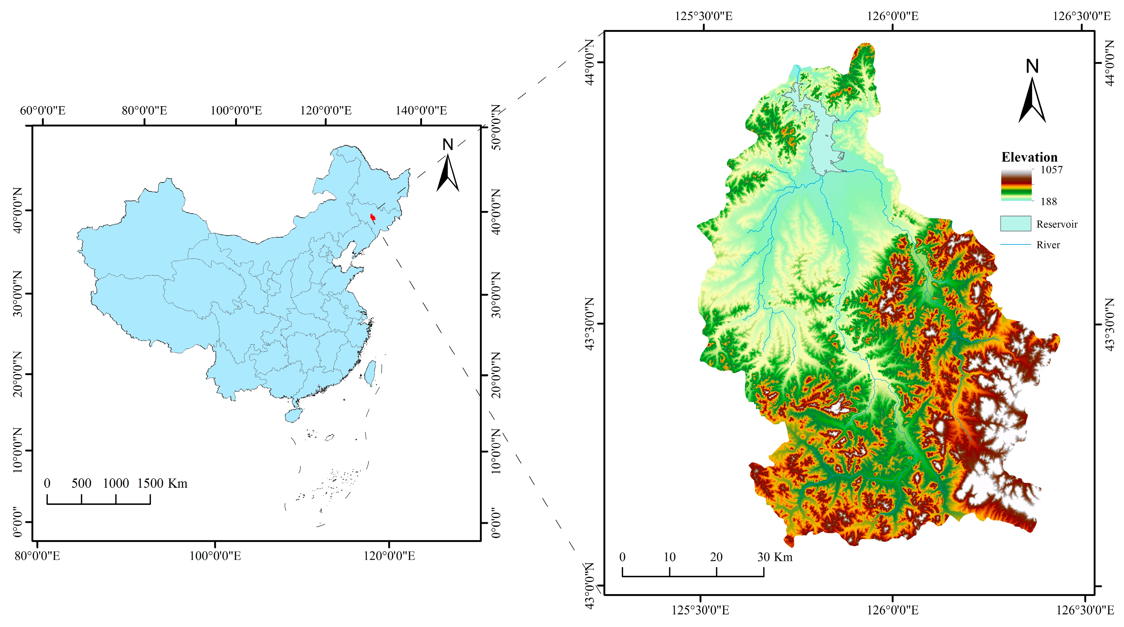
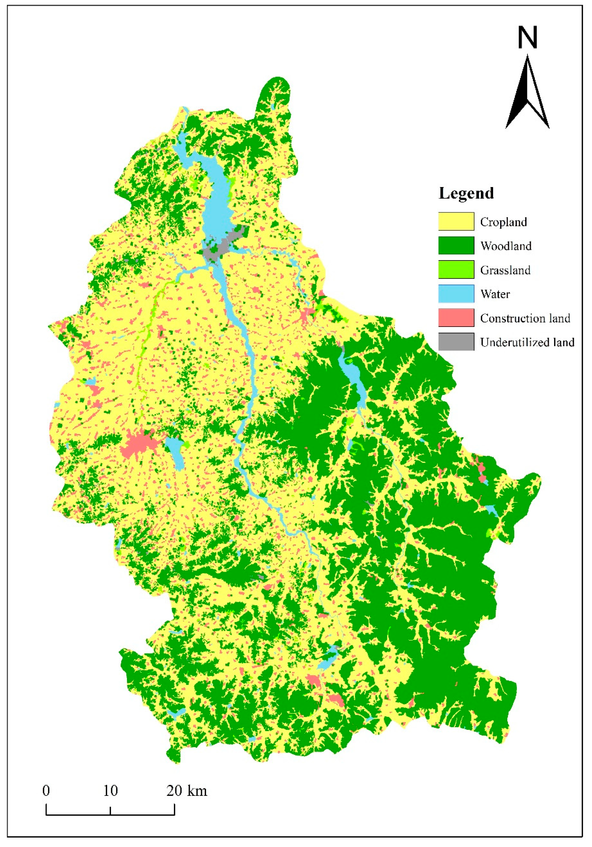
2.1. Study Area
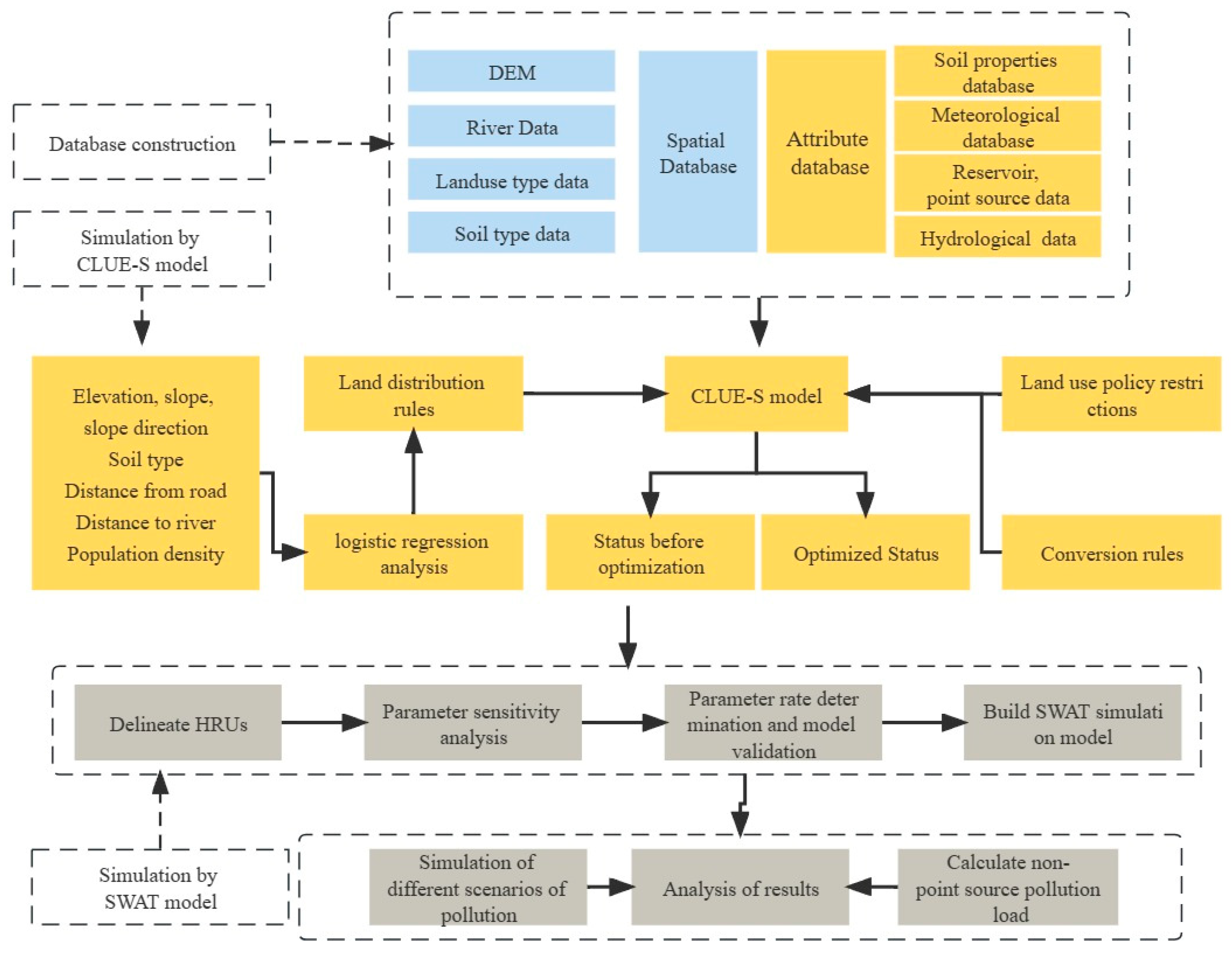
2.2. Model Approach
2.2.1. MODP Method
- (1)
- Selection of a time series, based on existing data, reflecting a specific time interval before and after applying the optimal design of the final model;
- (2)
- Determination of multi-objective decision variables, with the range of each class selected as the decision variable;
- (3)
- Construction of MODP constraints, based on land use characteristics and optimal allocation requirements, taking into account the needs and operability of a comprehensive, targeted management plan incorporating the benefits (social, economic, and ecological) of land use.
- (4)
- Construction of a multi-objective decision function for the establishment of a land use optimization model, based on specific objectives and designed to maximize the benefits (economic, social, and/or ecological). The objective function was expressed as:where is an abbreviation for subject to, which indicates constraints, is the ith objective function value, is the pre-determined desired value for each target, while are positive and negative deviation variables, indicating differences between actual values and values that exceed and fall short of the target values, respectively.
2.2.2. CLUE-S Model
- (1)
- Patterns of land distribution: we applied a logistic regression analysis to explore relationships between the drivers of each land type’s spatial distribution and its probable distribution, which was quantitatively described using the following regression equation:where is the probability of land use type i occurring on a particular raster image element, is the explanatory variable’s coefficient for each regression equation, and is the value for each driver of different land types.
- (2)
- Rules of land use transfer: a land transfer matrix and the elasticity of land use type conversion (ELAS) were used to set the rules of conversion between land types [38]. The ELAS parameter has a range of 0–1, and the value is positively correlated to the difficulty of converting a specified use type to other types: the smaller the value, the less stable the use and the easier it is to convert.
- (3)
- Calculating land demands: areas of land use can be predicted using the non-spatial module, or other models can be introduced [39]. In this study, we used the MODP approach.
- (4)
- Spatial allocation of land types: the CLUE-S spatial allocation module is based on the probable distributions of the land use types in a given area, using the formula:where is the total distribution probability of raster cell i for each land use type u, is the applicability of raster cell u to land type i derived from logistic regression analysis, is the conversion elasticity coefficient for land use type u, and is the specific iteration coefficient.
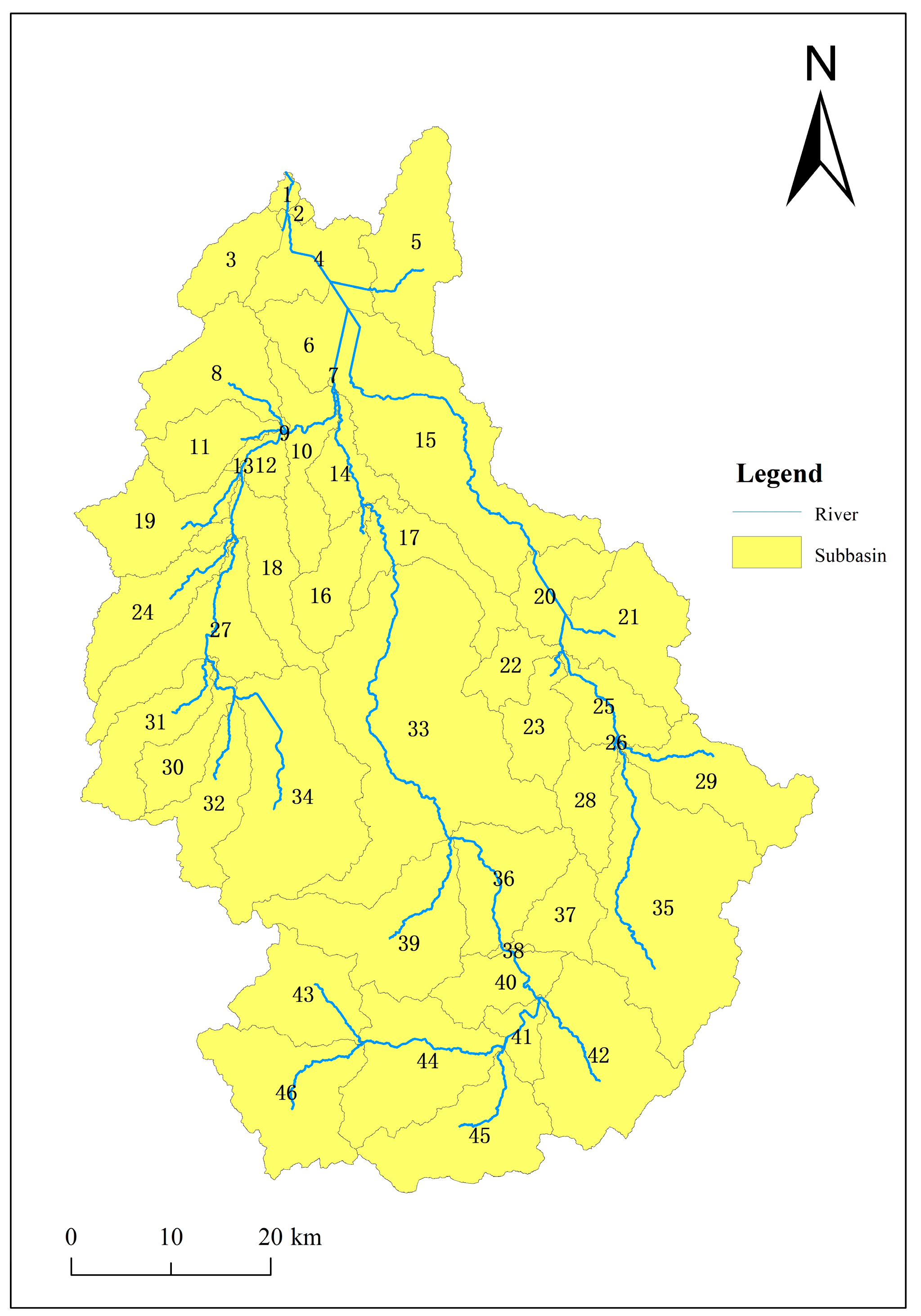
2.2.3. SWAT Model
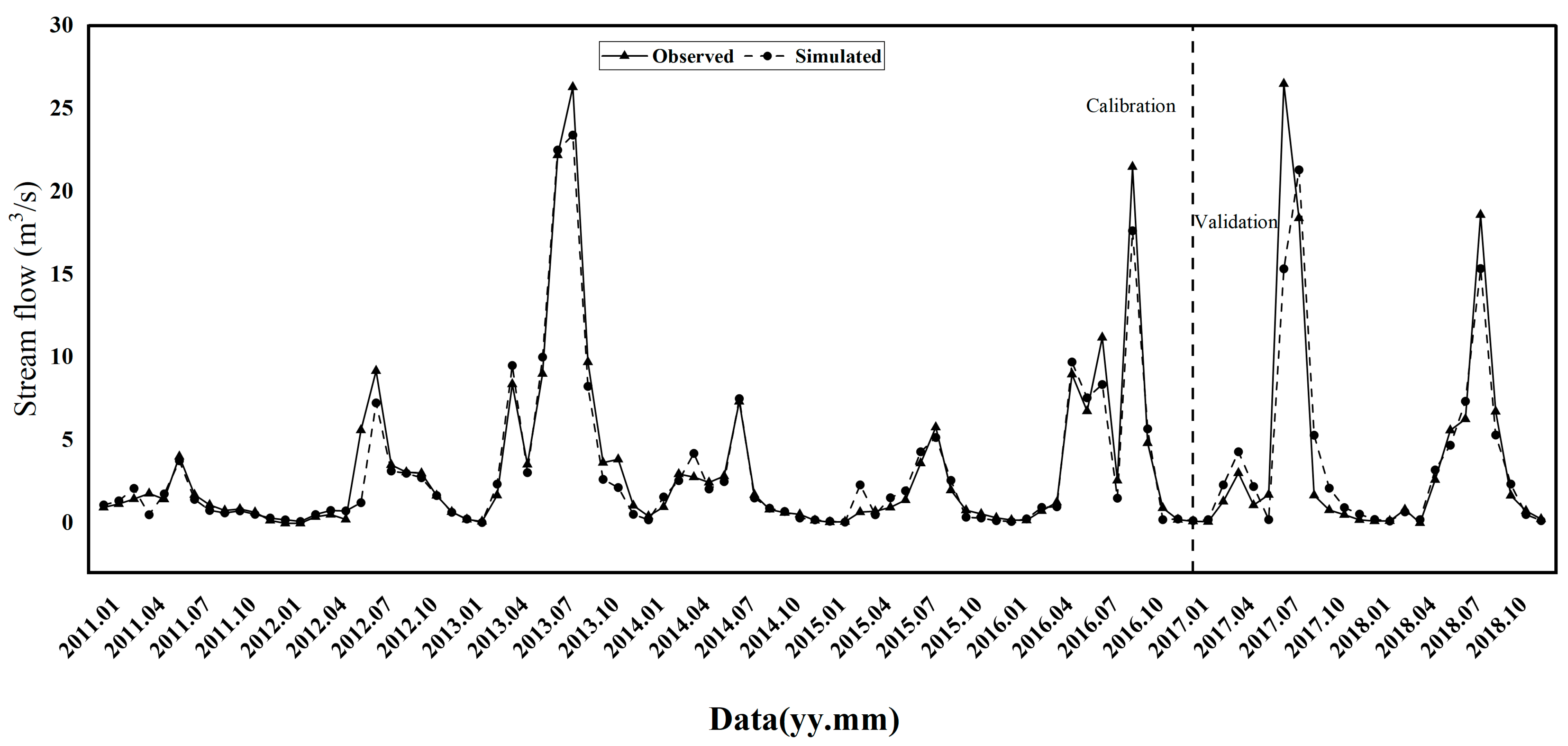
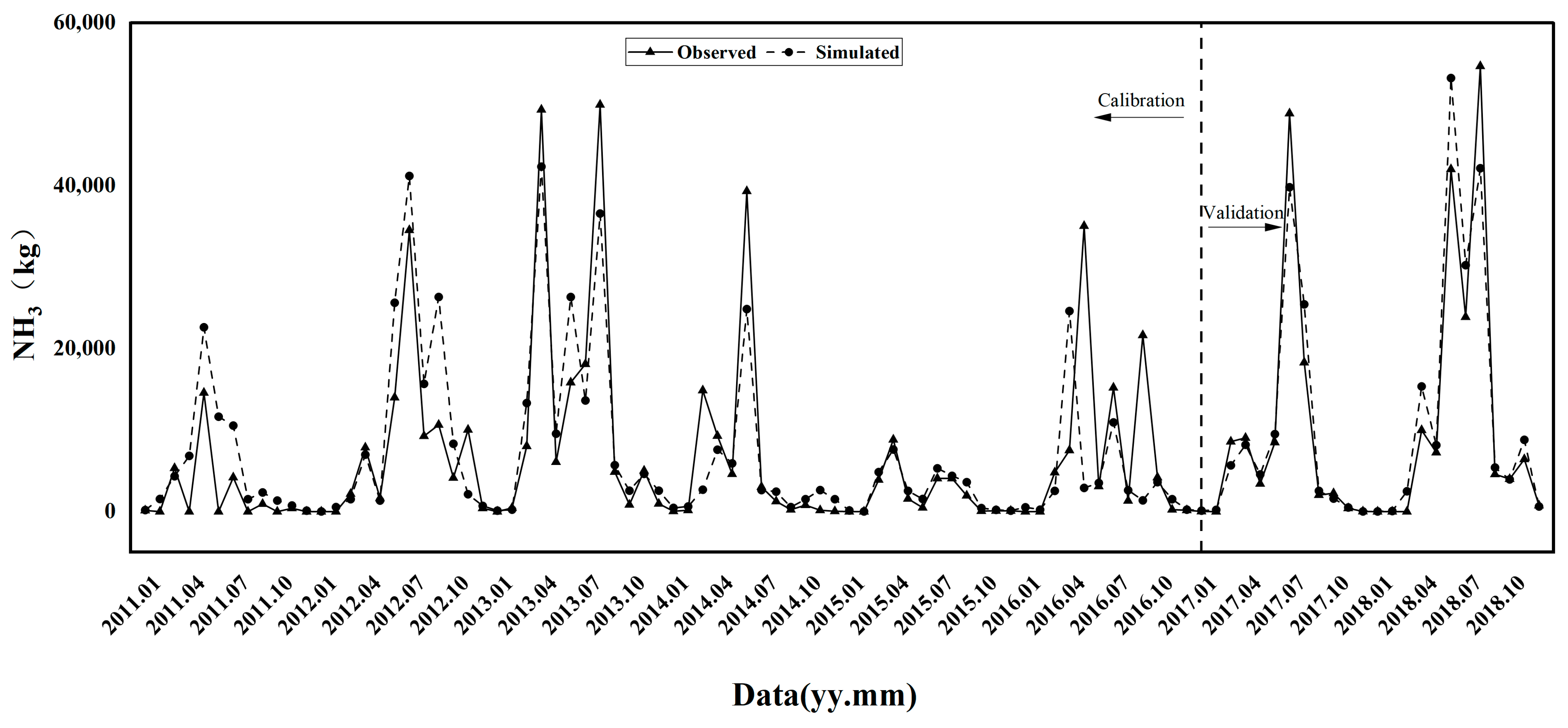
2.3. Calibration and Validation
2.4. Model Input Preparation
2.5. Model Execution
3. Results
3.1. Model Calibration and Performance Evaluation
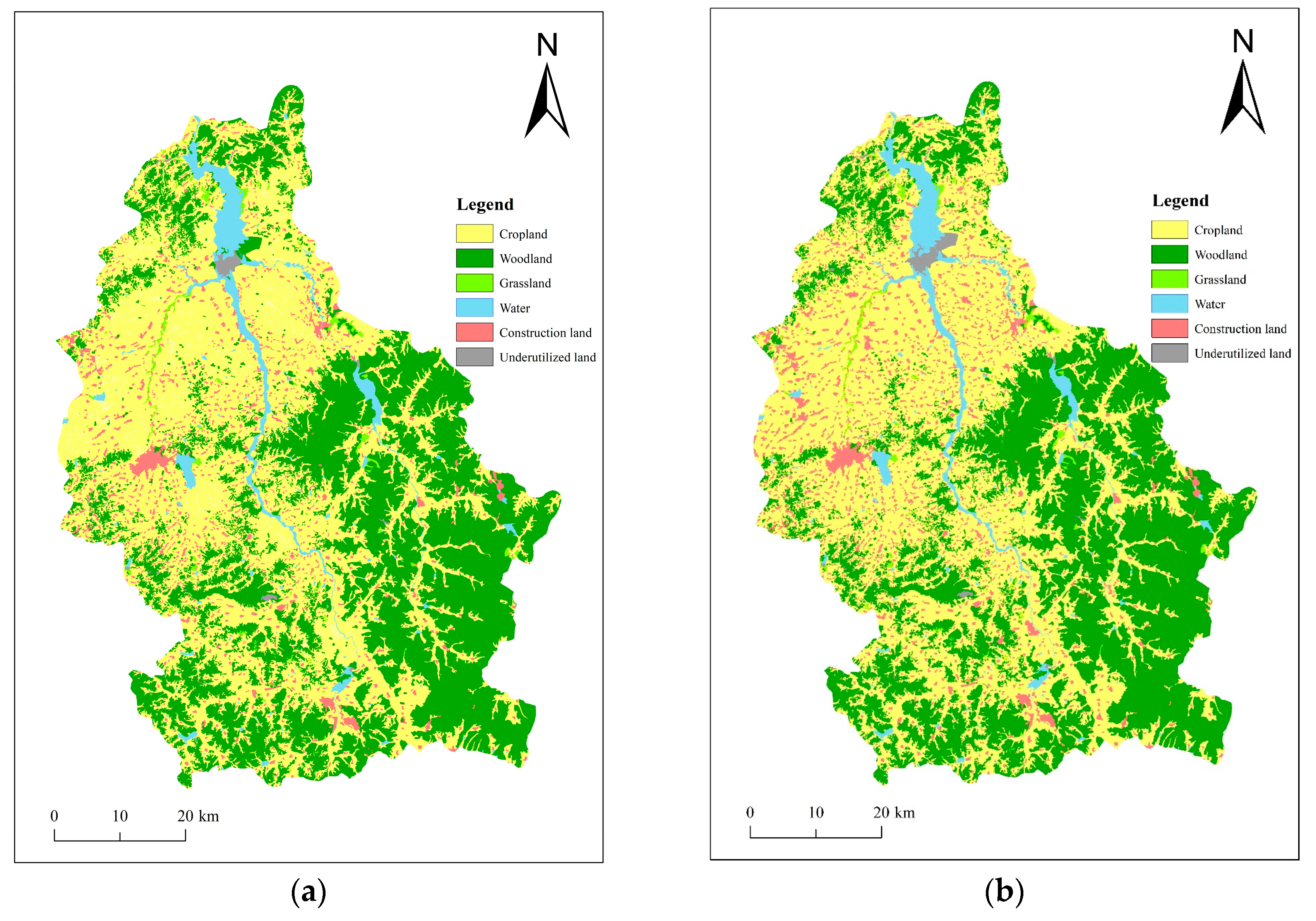
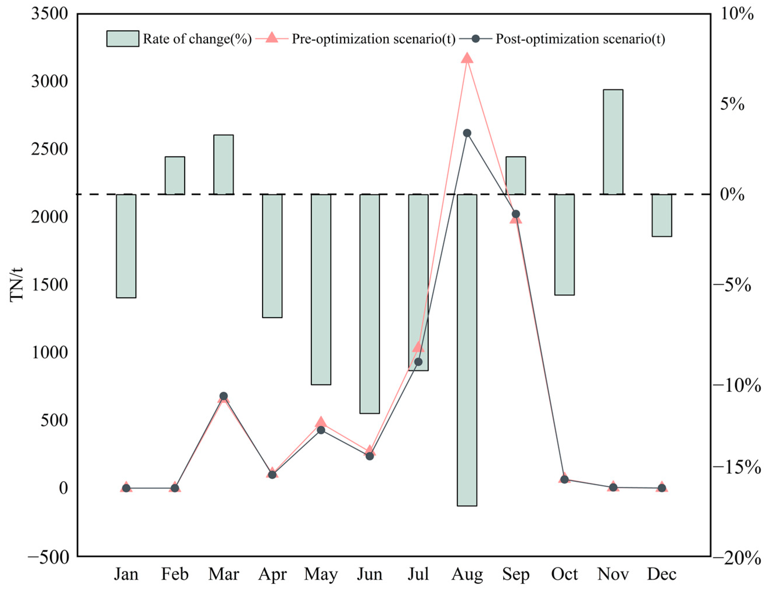
3.2. Land Use Optimization
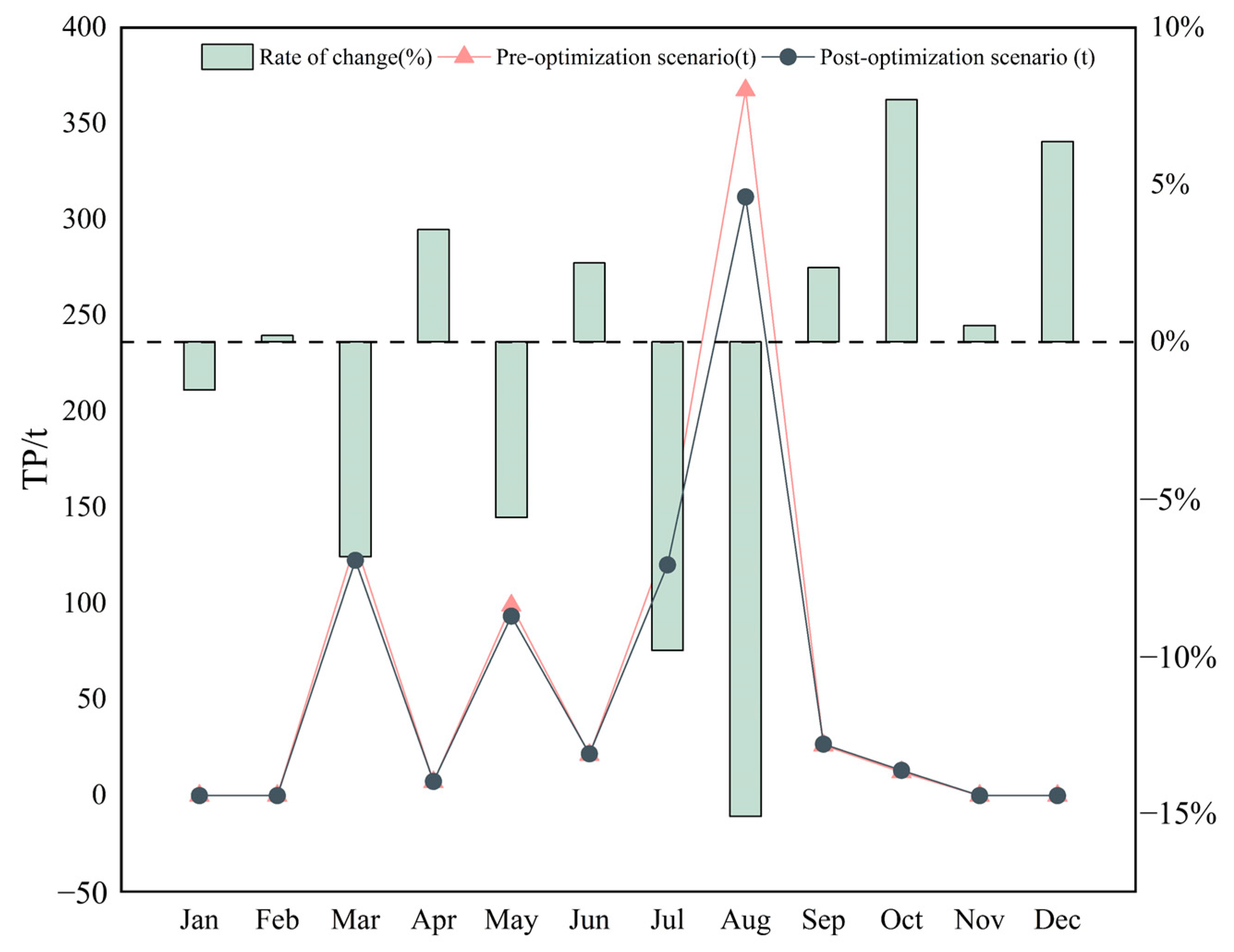
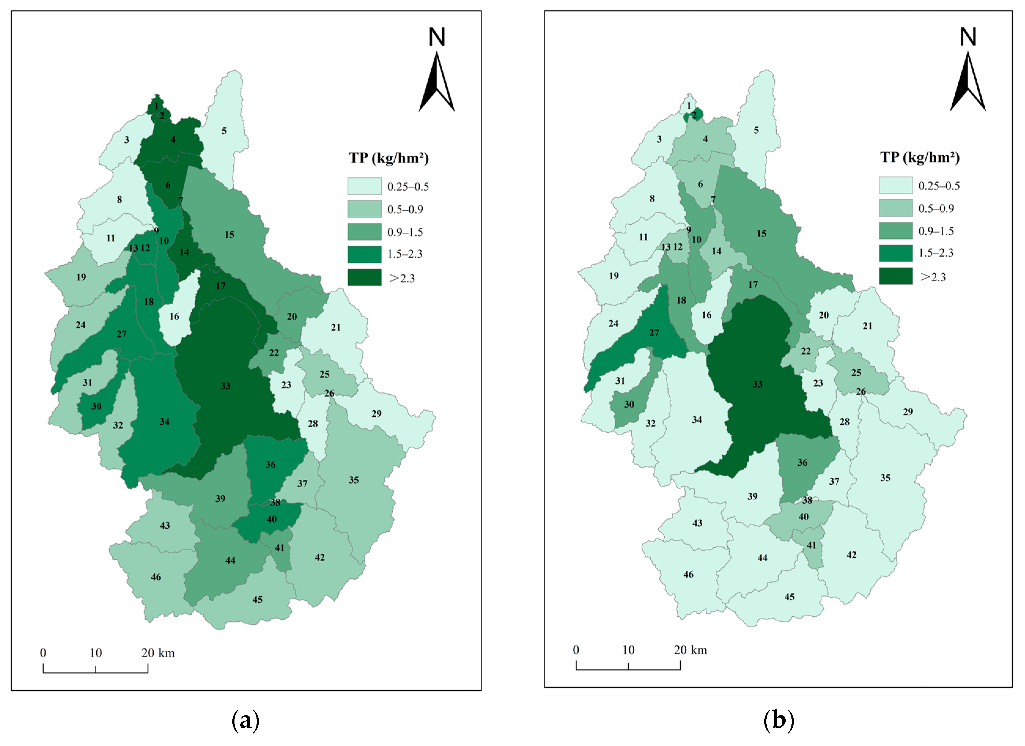
3.3. Comparison of Non-Point Source Pollution
4. Discussion
5. Conclusions
Author Contributions
Funding
Data Availability Statement
Conflicts of Interest
References
- Wang, Q.; Liu, R.; Men, C.; Guo, L. Application of genetic algorithm to land use optimization for non-point source pollution control based on CLUE-S and SWAT. J. Hydrol. 2018, 560, 86–96. [Google Scholar] [CrossRef]
- Huang, J.; Lin, X.; Wang, J.; Wang, H. The precipitation driven correlation-based mapping method (PCM) for identifying the critical source areas of nonpoint source pollution. J. Hydrol. 2015, 524, 100–110. [Google Scholar] [CrossRef]
- Luo, X.; Zheng, Y.; Lin, Z.; Wu, B.; Han, F.; Tian, Y.; Zhang, W.; Wang, X. Evaluating potential non-point source loading of PAHs from contaminated soils: A fugacity-based modeling approach. Environ. Pollut. 2015, 196, 1–11. [Google Scholar] [CrossRef] [PubMed]
- Li, T.; Bai, F.; Han, P.; Zhang, Y. Non-point source pollutant load variation in rapid urbanization areas by remote sensing, Gis and the L-THIA model: A casein Bao’an District, Shenzhen, China. Environ. Manag. 2016, 58, 873–888. [Google Scholar] [CrossRef] [PubMed]
- Xia, J.; Zhai, X.; Zhang, Y. Progress in the research of water environmental nonpoint source pollution models. Prog. Geogr. 2012, 31, 941–952. [Google Scholar]
- Huang, Q.; Shi, P.; He, C.; Li, X. Modelling land use change dynamics under different aridification scenarios in northern China. Acta Geogr. Sin. 2006, 61, 1299–1310. [Google Scholar] [CrossRef]
- Li, Q. Effects of correlated forecast errors on population forecast. Chin. J. Popul. Sci. 2017, 5, 86–95+128. [Google Scholar]
- Liu, J.; Zhang, C.; Xu, X.; Kuang, W.; Zhou, M.; Zhang, S.; Li, R.; Ya, C.; Xu, D.; Tun, S.; et al. Spatial patterns and driving forces of land use change in China in the early 21st century. Acta Geogr. Sin. 2009, 64, 1411–1420. [Google Scholar] [CrossRef]
- Batisani, N.; Yarnal, B. Uncertainty awareness in urban sprawl simulations: Lessons from a small US metropolitan region. Land Use Pol. 2009, 26, 178–185. [Google Scholar] [CrossRef]
- Boulange, J.; Watanabe, H.; Inao, K.; Iwafune, T.; Zhang, M.; Luo, Y.; Arnold, J. Development and validation of a basin scale model PCPF-1@SWAT for simulating fate and transport of rice pesticides. J. Hydrol. 2014, 517, 146–156. [Google Scholar] [CrossRef]
- Xu, L.; Li, Z.; Song, H.; Yin, H. Land-Use Planning for Urban Sprawl Based on the CLUE-S Model: A Case Study of Guangzhou, China. Entropy 2013, 15, 3490–3506. [Google Scholar] [CrossRef]
- Zhou, Y.; Min, X.; Yu, X.; Li, X. Characteristics of non-point source pollution in Shijiu Lake basin based on SWAT model. Sichuan Environ. 2021, 40, 186–191. [Google Scholar]
- Zhang, P.; Liu, Y.; Pan, Y.; Yu, Z. Land use pattern optimization based on CLUE-S and SWAT models for agricultural non-point source pollution control. Math. Comput. Model 2013, 58, 588–595. [Google Scholar] [CrossRef]
- Han, J.; Huang, G.; Zhang, H.; Li, Z.; Li, Y. Effects of watershed subdivision level on semi-distributed hydrological simulations: Case study of the SLURP model applied to the Xiangxi River watershed, China. Hydrol. Sci. J. 2013, 59, 108–125. [Google Scholar] [CrossRef]
- Cai, Y.; Liu, Y.; Yu, Z.; Verburg, P. Progress in spatial simulation of land use change—CLUE-S model and its application. Prog. Geogr. 2004, 23, 63–71. [Google Scholar]
- Parajuli, P.; Jayakody, P.; Sassenrath, G.; Ouyang, Y.; Pote, J. Assessing the impacts of crop-rotation and tillage on crop yields and sediment yield using a modeling approach. Agric. Water Manag. 2013, 119, 32–42. [Google Scholar] [CrossRef]
- Romano, G.; Abdelwahab, O.; Gentile, F. Modeling land use changes and their impact on sediment load in a Mediterranean watershed. Catena 2018, 163, 342–353. [Google Scholar] [CrossRef]
- Cao, K.; Huang, B.; Wang, S.; Lin, H. Sustainable land use optimization using Boundary-based Fast Genetic Algorithm. Comput. Environ. Urban Syst. 2012, 36, 257–269. [Google Scholar] [CrossRef]
- Stewart, T.; Janssen, R.; Van, H. A genetic algorithm approach to multiobjective land use planning. Comput. Oper. Res. 2004, 31, 2293–2313. [Google Scholar] [CrossRef]
- Stewart, T.; Janssen, R. A multiobjective GIS-based land use planning algorithm. Comput. Environ. Urban Syst. 2014, 46, 25–34. [Google Scholar] [CrossRef]
- Dai, X.; Zhou, Y.; Ma, W.; Zhou, L. Influence of spatial variation in land-use patterns and topography on water quality of the rivers inflowing to Fuxian Lake, a large deep lake in the plateau of southwestern China. Ecol. Eng. 2017, 99, 417–428. [Google Scholar] [CrossRef]
- Zeiger, S.; Hubbart, J. An assessment of mean areal precipitation methods on simulated stream flow: A SWAT model performance assessment. Water 2017, 9, 459. [Google Scholar] [CrossRef]
- Fu, B.; Yu, D.; Zhang, Y. The livable urban landscape: GIS and remote sensing extracted land use assessment for urban livability in Changchun Proper, China. Land Use Pol. 2019, 87, 104048. [Google Scholar] [CrossRef]
- Bai, L.; Xiu, C.; Feng, X.; Liu, D. Influence of urbanization on regional habitat quality: A case study of Changchun City. Habitat. Int. 2019, 93, 102024. [Google Scholar] [CrossRef]
- Guo, R.; Wu, T.; Wu, X.; Luigi, S.; Wang, Y. Simulation of urban land expansion under ecological constraints in Harbin-Changchun urban agglomeration, China. Chin. Geogr. Sci. 2022, 32, 438–455. [Google Scholar] [CrossRef]
- Xu, X.; Li, X.; Xiao, C.; Ou, M. Optimization of regional land use layout under different scenarios based on CLUE-S model. Acta Ecol. Sin. 2016, 36, 5401–5410. [Google Scholar] [CrossRef]
- Xie, H.; Chen, L.; Shen, Z. Assessment of agricultural best management practices using models: Current issues and future perspectives. Water 2015, 7, 1088–1108. [Google Scholar] [CrossRef]
- Zheng, H.; Shen, G.; Wang, H.; Hong, J. Simulating land use change in urban renewal areas: A case study in Hong Kong. Habitat Int. 2015, 46, 23–34. [Google Scholar] [CrossRef]
- White, M.; Harmel, R.; Arnold, J.; Williams, J. SWAT check: A screening tool to assist users in the identification of potential model application problems. J. Environ. Qual. 2014, 43, 208–214. [Google Scholar] [CrossRef]
- Phippen, S.; Wohl, E. An assessment of land use and other factors affecting sediment loads in the Rio Puerco watershed, New Mexico. Geomorphology 2003, 52, 269–287. [Google Scholar] [CrossRef]
- Nie, W.; Yuan, Y.; Kepner, W.; Nash, M.; Jackson, M.; Erickson, C. Assessing impacts of Landuse and Landcover changes on hydrology for the upper San Pedro watershed. J. Hydrol. 2011, 407, 105–114. [Google Scholar] [CrossRef]
- Xie, G.; Zhen, L.; Lu, C.; Xiao, Y.; Chen, C. Expert knowledge based valuation method of ecosystem services in China. J. Nat. Resour. 2008, 5, 911–919. [Google Scholar]
- Liu, M.; Li, C.; Hu, Y.; Sun, F.; Xu, Y.; Chen, T. Combining CLUE-S and SWAT models to forecast land use change and non-point source pollution impact at a watershed scale in Liaoning Province, China. Chin. Geogr. Sci. 2014, 24, 540–550. [Google Scholar] [CrossRef]
- Verburg, P.; Overmars, K. Combining top-down and bottom-up dynamics in land use modeling: Exploring the future of abandoned farmlands in Europe with the Dyna-CLUE model. Landsc. Ecol. 2009, 24, 1167–1181. [Google Scholar] [CrossRef]
- Strehmel, A.; Schmalz, B.; Fohrer, N. Evaluation of Land Use, Land Management and Soil Conservation Strategies to Reduce Non-Point Source Pollution Loads in the Three Gorges Region, China. Environ. Manag. 2016, 58, 906–921. [Google Scholar] [CrossRef] [PubMed]
- Ongley, E.; Zhang, X.; Yu, T. Current status of agriculture and non-point source pollution assessment in China. Environ. Pollut. 2010, 158, 1159–1168. [Google Scholar] [CrossRef] [PubMed]
- Shi, Z.; Huang, X.; Ai, L.; Fang, N.; Wu, G. Quantitative analysis of factors controlling sediment yield in mountainous watersheds. Geomorphology 2014, 226, 193–201. [Google Scholar] [CrossRef]
- Yang, Y.; Bao, W.; Liu, Y. Scenario simulation of land system change in the Beijing-Tianjin-Hebei region. Land Use Pol. 2020, 96, 104677. [Google Scholar] [CrossRef]
- Ullah, S.; Ali, A.; Iqbal, M.; Javid, M.; Imran, M. Geospatial assessment of soil erosion intensity and sediment yield: A case study of Potohar Region, Pakistan. Environ. Earth Sci. 2018, 77, 705. [Google Scholar] [CrossRef]
- Li, G.; Zhao, Z.; Wang, L.; Li, Y.; Li, Y. Optimization of ecological land use layout based on multimodel coupling. J. Urban Plan Dev. 2023, 149, 04022053. [Google Scholar] [CrossRef]
- Arnold, J.; Srinivasan, R.; Muttiah, R.; Williams, J. Large area hydrologic modeling and assessment part I: Model development. J. Am. Water Resour. Assoc. 1998, 34, 73–89. [Google Scholar] [CrossRef]
- Jiang, X.; Wang, L.; Ma, F.; Li, H.; Zhang, S.; Liang, X. Localization method for SWAT model soil database based on HWSD. Chin. Water & Wast. 2014, 30, 135–138. [Google Scholar] [CrossRef]
- Li, J.; Zhou, Z. Coupled analysis on landscape pattern and hydrological processes in Yanhe watershed of China. Sci. Total Environ. 2015, 505, 927–938. [Google Scholar] [CrossRef] [PubMed]
- Strauch, M.; Volk, M. SWAT plant growth modification for improved modeling of perennial vegetation in the tropics. Ecol. Model. 2013, 269, 98–112. [Google Scholar] [CrossRef]
- Panagopoulos, Y.; Makropoulos, C.; Baltas, E.; Mimikou, M. SWAT parameterization for the identification of critical diffuse pollution source areas under data limitations. Ecol. Model. 2011, 222, 3500–3512. [Google Scholar] [CrossRef]
- Fu, Y.; Zang, W.; Dong, F.; Fu, M.; Zhang, J. Yield calculation of agricultural non-point source pollutants in Huntai River Basin based on SWAT model. Trans. Chin. Soc. Agric. Eng. 2016, 32, 1–8. [Google Scholar] [CrossRef]
- Wu, H.; Chen, B. Evaluating uncertainty estimates in distributed hydrological modeling for the Wenjing River watershed in China by GLUE, SUFI-2, and Para Sol methods. Ecol. Eng. 2015, 76, 110–121. [Google Scholar] [CrossRef]
- Briak, H.; Moussadek, R.; Aboumaria, K.; Mrabet, R. Assessing sediment yield in Kalaya gauged watershed (Northern Morocco) using GIS and SWAT model. Int. Soil Water Conserv. Res. 2016, 4, 177–185. [Google Scholar] [CrossRef]
- Li, Q.; Zhang, J.; Gong, H. Hydrological simulation and parameter uncertainty analysis using SWAT model based on SUIF-2 algorithm for Guishuihe River Basin. J. China Hydrol. 2015, 35, 43–48. [Google Scholar]
- Palao, L.; Dorado, M.; Anit, K.; Lasco, R. Using the soil and water assessment tool (SWAT) to assess material transfer in the layawan watershed, Mindanao, Philippines and its implications on payment for ecosystem services. J. Sustain. Devel. 2013, 6, 73–88. [Google Scholar] [CrossRef]
- Liu, R.; Wang, Q.; Xu, F.; Men, C.; Guo, L. Impacts of manure application on SWAT model outputs in the Xiangxi River watershed. J. Hydrol. 2017, 555, 479–488. [Google Scholar] [CrossRef]
- Reza, A.; Eum, J.; Jung, S.; Choi, Y.; Owen, J.; Kim, B. Export of non-point source suspended sediment, nitrogen, and phosphorus from sloping highland agricultural fields in the East Asian monsoon region. Environ. Monit. Assess. 2016, 188, 692. [Google Scholar] [CrossRef] [PubMed]
- Grusson, Y.; Sun, X.; Gascoin, S.; Sauvage, S.; Raghavan, S.; Anctil, F.; Sáchez-Pérez, J. Assessing the capability of the SWAT model to simulate snow, snow melt and streamflow dynamics over an alpine watershed. J. Hydrol. 2015, 531, 574–588. [Google Scholar] [CrossRef]
- Yang, W.; Su, B.; Luo, Y.; Zhang, Q. method of non-point source pollution load accounting by SWAT model under influence of point-source discharge. Water Resour. Power 2013, 31, 21–24. [Google Scholar]
- Sinha, R.; Eldho, T.; Subimal, G. Assessing the impacts of land cover and climate on runoff and sediment yield of a river basin. Hydrol. Sci. J. 2020, 65, 2097–2115. [Google Scholar] [CrossRef]
- Meng, X.; Zhang, X.; Yang, M.; Wang, H.; Chen, J.; Pan, Z.; Wu, Y. Application and Evaluation of the China Meteorological Assimilation Driving Datasets for the SWAT Model (CMADS) in Poorly Gauged Regions in Western China. Water 2019, 11, 2171. [Google Scholar] [CrossRef]
- Yan, X.; Lu, W.; An, Y.; Dong, W. Assessment of parameter uncertainty for non-point source pollution mechanism modeling: A Bayesian-based approach. Environ. Pollut. 2020, 263, 114570. [Google Scholar] [CrossRef]
- Li, H.; Zhang, J.; Zhang, S.; Zhang, W.; Zhang, S.; Yu, P.; Song, Z. A framework to assess spatio-temporal variations of potential non-point source pollution risk for future land-use planning. Ecol. Indic. 2022, 137, 108751. [Google Scholar] [CrossRef]
- Zhang, L.; Lu, W.; Hou, G.; Gao, H.; Liu, H.; Zheng, Y. Coupled analysis on land use, landscape pattern and nonpoint source pollution loads in Shitoukoumen Reservoir watershed, China. Sustain. Cities Soc. 2019, 51, 101788. [Google Scholar] [CrossRef]


| Coding of Land Use | Type of Land Use | AUC Value |
|---|---|---|
| 0 | Cropland | 0.928 |
| 1 | Woodland | 0.962 |
| 2 | Grassland | 0.824 |
| 3 | Water | 0.857 |
| 4 | Construction land | 0.931 |
| 5 | Underutilized land | 0.829 |
| Data Type | Station | R2 (Calibration Period) | ENS (Calibration Period) | R2 (Validation Period) | ENS (Validation Period) |
|---|---|---|---|---|---|
| Runoff | Xinan | 0.78 | 0.71 | 0.76 | 0.72 |
| Xingxingshao | 0.73 | 0.71 | 0.71 | 0.66 | |
| Chang ling | 0.80 | 0.76 | 0.77 | 0.73 | |
| Yantong shan | 0.82 | 0.77 | 0.79 | 0.75 | |
| Contaminants | Xinan | 0.80 | 0.76 | 0.76 | 0.73 |
| Yantong shan | 0.74 | 0.71 | 0.74 | 0.63 |
| Land Use Type | Cropland | Woodland | Grassland | Water | Construction Land | Underutilized Land |
|---|---|---|---|---|---|---|
| Before optimization (ha) | 247,845 | 186,881.75 | 3884.5 | 16,719.25 | 31,158.25 | 2766.25 |
| After optimization (ha) | 247,895 | 195,386.6 | 3822.5 | 16,694.7 | 24,626.4 | 829.8 |
| Change in area (ha) | 50 | 8504.85 | −62 | −24.55 | −6531.85 | −1936.45 |
| Rate of change (%) | 0.02% | 4.55% | −1.60% | −0.15% | −20.96% | −70.00% |
Disclaimer/Publisher’s Note: The statements, opinions and data contained in all publications are solely those of the individual author(s) and contributor(s) and not of MDPI and/or the editor(s). MDPI and/or the editor(s) disclaim responsibility for any injury to people or property resulting from any ideas, methods, instructions or products referred to in the content. |
© 2023 by the authors. Licensee MDPI, Basel, Switzerland. This article is an open access article distributed under the terms and conditions of the Creative Commons Attribution (CC BY) license (https://creativecommons.org/licenses/by/4.0/).
Share and Cite
Li, G.; Chang, L.; Li, H.; Li, Y. Modeling the Impact of Land Use Optimization on Non-Point Source Pollution: Evidence from Chinese Reservoir Watershed. Land 2024, 13, 18. https://doi.org/10.3390/land13010018
Li G, Chang L, Li H, Li Y. Modeling the Impact of Land Use Optimization on Non-Point Source Pollution: Evidence from Chinese Reservoir Watershed. Land. 2024; 13(1):18. https://doi.org/10.3390/land13010018
Chicago/Turabian StyleLi, Guanghui, Lei Chang, Haoye Li, and Yuefen Li. 2024. "Modeling the Impact of Land Use Optimization on Non-Point Source Pollution: Evidence from Chinese Reservoir Watershed" Land 13, no. 1: 18. https://doi.org/10.3390/land13010018