New Insights into Urbanization Based on Global Mapping and Analysis of Human Settlements in the Rural–Urban Continuum

Abstract

The clear boundary between urban and rural areas is gradually disappearing, and urban and rural areas are two poles of a gradient with many continuous human settlements in between, which is a concept known as the rural–urban continuum. Little is known about the distribution and change trajectories of the various types in the rural–urban continuum across the globe. Therefore, using global land-cover data (FROM-GLC Plus) and global population data (Worldpop) based on the decision-making tree method, this study proposed a method and classification system for global rural–urban continuum mapping and produced the mapping results on a global scale in the Google Earth Engine platform. With the expansion of built-up areas and the increase in population, the global human settlements follow the pattern that develops from wildland to villages (isolated—sparse—dense), and then to towns (sparse—dense), and finally to urban areas (edge—center). From a regional perspective, there are some obvious differences: Africa is dominated by sparse villages; Asia has the highest proportion of densely clustered towns; the proportion of dense villages in Europe is high. Rural–urban continuum mapping and analysis provide a database and new insights into urbanization and differences between urban and rural areas around the world.

1. Introduction

A wide variety of human settlements have been created as the result of the great human transformation of natural landscapes [1,2]. Urban areas are the most intense transformation of natural landscapes among all the human settlements, and a common urban–rural dichotomy refers to human settlements outside urban areas as rural areas [3,4]. Increasing urbanization has led to the formation of complex geographies [5]. Many regional studies have found the limitations of a simple urban–rural dichotomy to reveal the real situation of human settlements [6,7,8]. In addition, the criteria and thresholds for dividing urban and rural areas vary widely in each country and region [9]. The clear boundary between urban and rural areas is gradually disappearing; urban and rural areas are two poles of a gradient with many continuous transitional landscapes in between [4].

This concept, which emphasizes the continuous transitional landscapes between urban and rural areas, is called the rural–urban continuum. Since the early 20th century, the theory of a rural–urban continuum has been continuously enriched, developed, and matured in practice [3,10,11,12,13,14]. In 1970, the United States Department of Agriculture began to develop the Rural–Urban Continuum Code (RUCC) to classify counties [15]. Similarly, landscape features of the rural–urban continuum have been noted in several regions of the globe, including Europe [6,8], China [16,17], and India [7]. In Europe, much of physical territory is regarded as areas between urban and rural, and there have been proposed definitions and mapping criteria for these peri-urban areas [6,8]. In addition, the traditional Chinese settlement system has been seen as a town–village–field continuum [16]. There are studies that have defined the settlement system in China and mapped its change trajectory between 1990 and 2010 [17]. However, the criteria and thresholds for dividing urban and rural areas vary widely in each country and region. Empirical analysis and conceptual comparisons show that towns and cities are likely to be classified as rural areas in Africa and Asia, and as urban areas in other parts of the world [18]. Therefore, it is necessary to construct a unified classification system on a global scale to define and map the various types of areas in the rural–urban continuum. Globally, the Global Human Settlement Layer (GHSL) produced by the Joint Research Centre (JRC) of the European Commission has provided mapping results at 5-year intervals beginning in 1975 and predicts changes over the next decade [19].

The concept of the rural–urban continuum and its extensive practice provide a new perspective for the study of urban areas and the urbanization process. In the classification results of remote sensing images, the data basis for a large number of analyses, the area mainly covered by impervious pixels is assigned to the built-up area, while the other areas are regarded as non-built-up areas [4]. There have been many studies that have estimated the distribution of urban areas around the world and the populations that live in them. It is estimated that about 2% of the terrestrial land can be characterized as urban [20], and these urban areas contain more than half of the global population, which is expected to increase in the near future [21]. In addition, there is also an overall understanding of urban growth rates and regional differences. Gong et al. mapped global artificial impervious areas (GAIAs) and analyzed the trend of urban expansion in various countries and regions around the world [22]. Liu et al. analyzed global urban change from 1985 to 2015 and found that global urban extent has expanded at an unprecedented rate that is notably faster than that of population growth [23]. However, based on the perspective of the urban–rural continuum, urban areas are no longer just a single type, but a state of continuous development. From the perspective of the rural–urban continuum, the relationship between urban land expansion and population growth also needs to be viewed more carefully. It is also meaningful to understand the distribution, size, population, and historical trends of various types of human settlements from the rural–urban continuum perspective across the globe.

Furthermore, in the system of the urban–rural continuum, urbanization is no longer just the transformation of non-built-up area to built-up area, but the complex process of rural–urban development, which should be studied in depth. There are studies that compare urban patterns and urbanization in different regions [24,25,26]. Schmitt et al. found that Germany’s metropolitan areas are characterized by numerous small, equal-sized clusters, while the United States contains one large and dominant center [24]. An uneven distribution of urbanization was observed at different economic levels manifested by varying rates of population growth and expansion of built-up areas [25]. Tian et al. found that the dominant characteristics of urbanization in Asia and Africa are increased population density and built-up patch density, while urbanization in Europe and North America took a rather steady pace, combined with widespread greening [26]. It is said that human settlement changes follow multiple different trajectories in different locations, in small and incremental steps toward urban areas [17]. However, the specific characteristics of the development process have not yet provided conclusions on a global scale and still need to be systematically and comprehensively analyzed from the rural–urban continuum.

To understand the developing patterns and rules of human settlements, different types of human settlements must be defined and mapped in a continuous trajectory. Additionally, the study of human settlements has great implications, such as the disturbance of human activities in nature [27,28], equality of access to services [3], and the effectiveness of resource utilization [29,30]). Therefore, this study proposed a classification system for global rural–urban continuum mapping and produced global maps in the Google Earth Engine platform using global land-cover data (FROM-GLC Plus) and global population data (Worldpop) based on the decision-making tree method. We further analyzed the current state of the rural–urban continuum (distribution, area, unit number, population, etc.) as well as historical trends over the past two decades and tried to understand the developing patterns and rules of human settlements and their geographic differentiation.

2. Materials and Methods

2.1. A Review of the Human Settlement Classification Systems

Unlike a clearly defined and widely acknowledged classification system in land-cover mapping such as dividing land categories into cropland, impervious, forest, and so on, how to generate a continuous and integrated classification system and accurately capture the differences among all types of human settlements still remains a problem. Population is a commonly used indicator when separating urban and rural areas [31]. GHSL combines population size and population density thresholds to capture the full settlement hierarchy (including urban center, dense urban cluster, semi-dense urban cluster, suburban grid cell, rural cluster, low-density rural grid cell, very low-density grid cell) [32]. Population as a classification indicator for human settlements does not apply to areas with high population density but to low levels of urbanization, such as in India [33]. Built-up areas are another commonly chosen indicator, which are regarded as the most direct modification of the natural surface by human activities. Based on built-up land, cluster density, and cluster size, Li et al. divided China’s land surface into large cities, urban landscapes, suburban landscapes, densely clustered towns, sparsely clustered towns, dense villages, sparse villages, isolated villages, and deep rural areas [17]. However, this classification system cannot avoid errors in areas where the indicators of built-up area and actual resident population are inconsistent, such as ghost cities [34] and hollow villages [35]. Therefore, population, built-up areas, and other indicators should be combined to provide an integrated classification framework.

The classification system and methodology in the above studies are of great reference value [17,32], but these classification systems only distinguish the various types of urban to rural landscapes and cannot reflect the gradual transition of rural to wilderness. Ellis et al. mapped the anthropogenic biomes based on population density and land use in a long time series (from 10,000 BC to 2015 AD) [1]. In this classification system, non-built-up land was first classified into cropland, rangeland, woodland, etc., and then further classified them into residential, populated, and remote according to the level of population density. Moreover, time continuity, spatial scope, spatial resolution, and the resolution of the classification system greatly affect the use of data products. Data products from Li et al. (2019) focused on China and were mapped in ten-year intervals [17]. The anthropogenic biomes product has global spatial coverage and historical continuity; it still has the problem of coarse spatial resolution (10 km) whose use is limited, especially in the last 20 years. Although GHSL covers the global space scope and provides data series at five-year intervals, it ignores the detailed transitional change from rural to wild (

Table 1. Comparison of datasets in human settlement mapping studies.

Dataset	Classification System	Time Period	Spatial Coverage	Spatial Resolution
Li et al. (2019) [17]	Rural–urban continuum	1990, 2000, 2010	China	2 km
GHSL	Rural–urban continuum	1975–2030	World	1 km
Anthropogenic Biomes	Urban, rural–wild continuum	10,000 BCE—2015 CE	World	10 km
Mu et al. (2022) [36]	Unified Values from 1–10, but 3 classes	2000–2018	World	1 km
Tian et al. (2022) [26]	Urbanization pattern types	1975, 1990, 2015	World	5 km

). Mu et al. developed a global annual human footprint dataset from 2000 to 2018 with a resolution of 1 km, dividing the land surface into the wilderness (Human Footprint < 1), the intact areas (Human Footprint < 4), and the highly modified region (Human Footprint ≥ 4) [36]. Although continuous values are assigned to the land grids representing the intensity of human activity, they are roughly grouped into three categories, limiting further use of the dataset. Tian et al. used population, built-up land, and greenness to classify global urbanization types into greenness loss, steady urbanization, population decrease, and so on [26]. Although the change types of human settlement have been interpreted in various aspects, a clear mapping result to explain the current state of human settlement is still lacking.

Therefore, we adopted a classification system that integrates features of previous studies. As for the rural–urban continuum, we classified land as urban centers, urban landscapes, densely clustered towns, sparsely clustered towns, dense villages, sparse villages, and isolated villages. As for the cropland, rangeland, and woodland, we further classified them into residential, populated, and remote according to the level of population density. Other land types include wildland, water, and ice snow.

2.2. Data and Processing

Data used in human settlements mapping include the following three types (

Table 2. Datasets used in human settlement mapping and analysis.

Dataset Type	Name	Spatial Resolution	Duration	Usage
Land cover	FROM-GLC-Plus	30 m	2000–2020	Mapping
Population	Worldpop	100 m	2000–2020	Mapping
Elevation	SRTM	30 m	/	Mapping
Settlements samples	World Cities Database	/	/	Analysis
GDP	Gridded Global GDP dataset	5 arc-min	1990–2015	Analysis
Administrative boundaries	GeoBoundaries	/	/	Analysis

):

Global annual 30 m land-cover dataset. The land-cover dataset used in this study is FROM-GLC-Plus, which describes the dynamics of global land-cover change from 2000 to 2020 and divides the global land cover into the following 10 categories: cropland, forest, grassland, shrubland, wetland, water, tundra, impervious surface (built-up), bare land, snow and ice, with high spatial and temporal resolution [37].

Global population dataset. This study used Worldpop, which decomposed census-based count results into 100 m resolution grid cells using machine learning methods and the relationship between population density and a series of geospatial layers [38].

Global digital elevation data from the Shuttle Radar Topography Mission (SRTM), provided by NASA JPL laboratory, is at 1 arc second resolution (approximately 30 m) [39].

There are an additional three datasets helping us to analyze the final mapping result:

World Cities Database. This is a simple, accurate, and up-to-date database of all the populated places in the world (about 4.3 million). It is built from the ground up using authoritative sources such as the NGIA, US Geological Survey, US Census Bureau, and NASA (Online resources: https://simplemaps.com/data/world-cities, accessed on 13 August 2023).

Gridded Global GDP dataset. This provides annual gridded datasets for GDP per capita (PPP) and total GDP (PPP) for the whole world at 5 arc-min resolution for the 25-year period of 1990–2015 [40]. To provide a consistent product over time and space, the sub-national data were only used indirectly, scaling the reported national value and thus remaining representative of the official statistics.

Global Database of Political Administrative Boundaries (GeoBoundaries) is an online, open license resource of boundaries for every country in the world. All boundary types were ingested and include the following, with admin level varying from 0–4 (online resources: https://www.geoboundaries.org/, accessed on 13 August 2023) [41]. Here, we used political administrative boundaries with admin level varying from 0–2.

All the data need to be at the same resolution. Therefore, the global annual 30 m land-cover dataset was resampled at 1 km scale to calculate the proportion of each land-cover type on a 1 km grid, the global population 100 m dataset was resampled at 1 km scale to calculate the total population on a 1 km grid, and global slope data were calculated based on SRTM digital elevation data using terrain analysis algorithms in the Google Earth Engine [42].

2.3. Method

In order to better reflect the gradient difference in human activities’ intensity among the various types of human settlements, we calculated indicators based on population and land-cover datasets, including built-up density, population density, population size, etc. These indicators have proven to be effective in mapping the gradient difference between urban and rural areas in previous studies [1,17,19,26,43].

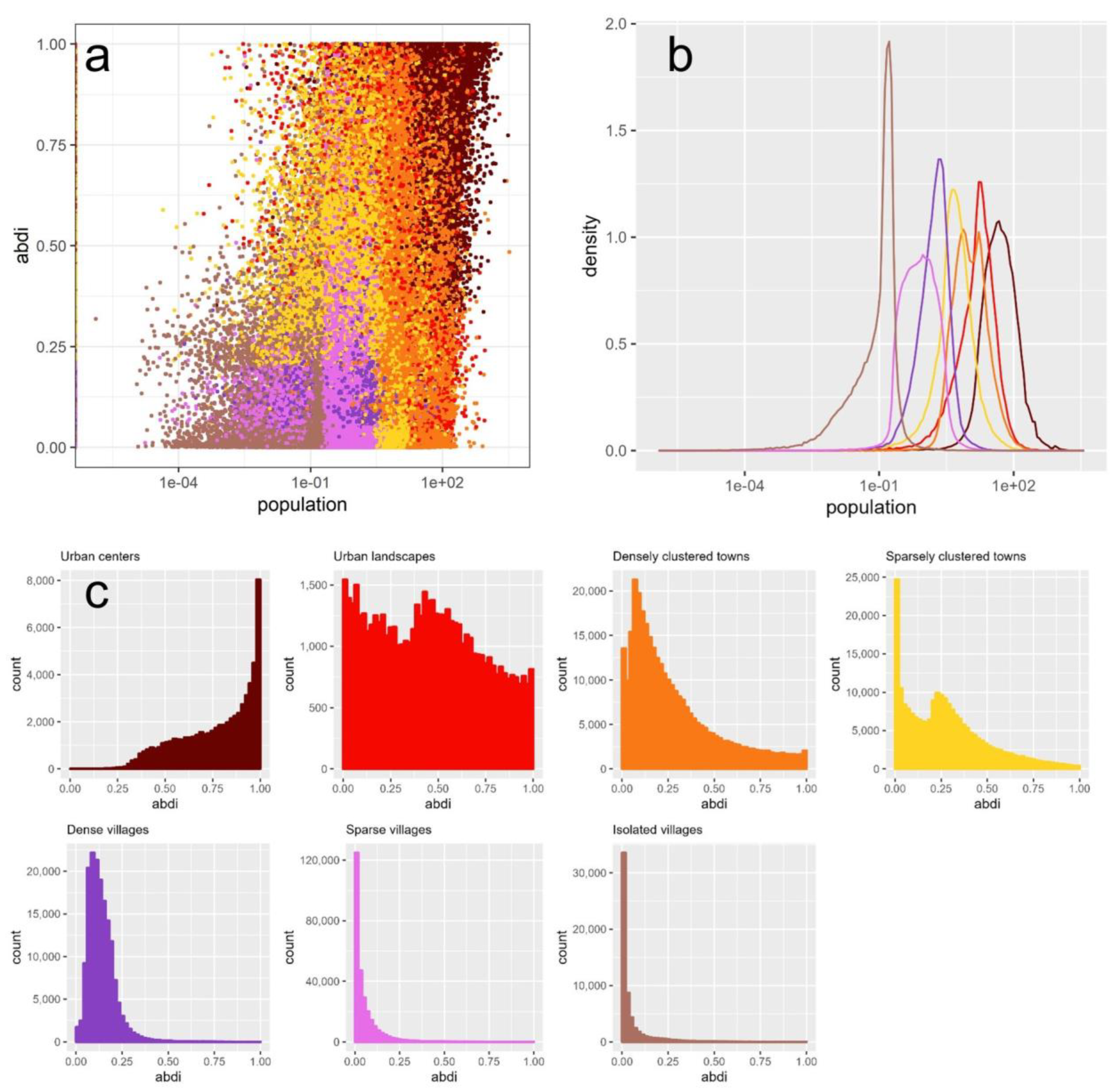
2.3.1. Index Calculation Based on Population and Built-Up Area

(1)

ABDI (Adjusted built-up density index)

Based on the global slope data and land-cover dataset, suitable construction land was defined as all areas that are not water or permanent snow and that have a slope that does not exceed 25% [17]. The 25% threshold is based on previous studies in China, which indicate that areas with a slope greater than 25% are not suitable for construction. The proportion of the suitable construction area was calculated at the scale of 1 km. ABDI was defined as the proportion of impervious surface (built-up area) divided by the proportion of suitable construction area at the 1 km scale. Li et al. defined the four intervals divided by ABDI at the three thresholds of 0.35, 0.2, and 0.05 as the density differences of built-up areas in urban areas, suburban/towns, villages and deep rural areas [17].

(2)

Spatial connectivity indicators

First, the parts larger than 1500, 300, and 20 of the global 1 km population grid were selected and exported separately to generate three different grid layers, which are respectively used as the partition thresholds of the 1 km population grid for urban areas, towns, and villages [32]. Spatial connectivity analysis was further used to calculate the number of connected grids in a cluster. More specifically, functions in the Google Earth Engine (GEE) were used to generate an image where each pixel contains the number of 4-connected or 8-connected neighbors (including itself). The image of the connected grid count was used to distinguish whether the total population reached the above standard. An urban grid cluster was defined as a cluster with connected grids of more than 1500 people and a total population of more than 50,000 people, which means this cluster must contain more than 34 grids. Similarly, a town grid cluster was defined as a cluster with connected grids of more than 300 people and a total population of more than 5000 people (more than 17 grids). Village grid clusters were defined as clusters with connected grids of more than 20 people and a total population of more than 100 people (more than 5 grids).

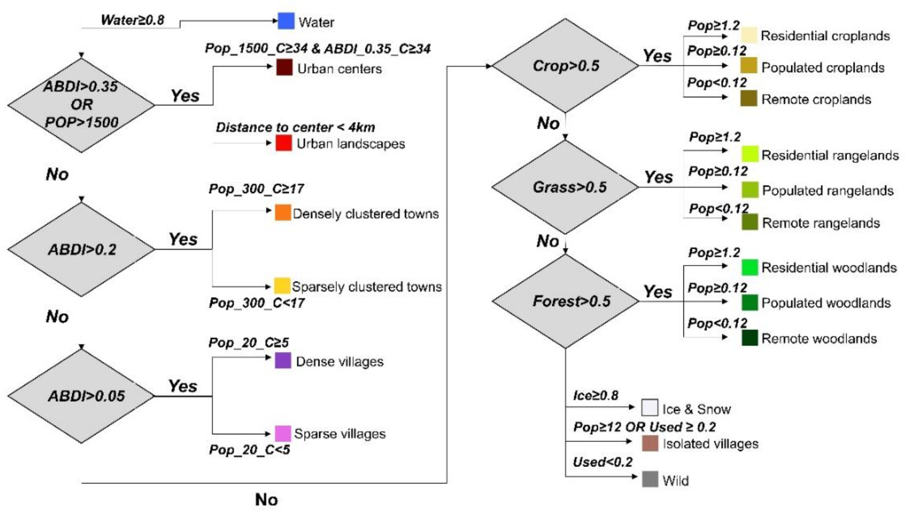
2.3.2. Construction of Classification Decision Tree

In this part, different types of human settlements were defined one by one by overlapping layers, basically from urban to rural and then to wild. Layers were stacked according to the order in Figure 1. Later defined types were defined to an extent out of the earlier defined type and would not cause overlap or conflict. The determination of threshold value referred to the previous work, and the specific situation was explained in Section 2.3.1.

First, areas with a water proportion greater than 0.8 were defined as water. And then grids with an ABDI greater than 0.35 or a population of more than 1500 were defined as urban areas. The urban center was defined as a cluster of more than 34 connected grids whose ABDIs were greater than 0.35 and population more than 1500. That is, the urban center had a total population of more than 50,000 people. The remaining urban areas within 4 km from the urban center were defined as urban landscapes (Figure 1).

Areas with ABDIs greater than 0.2 were defined as town areas; densely clustered towns were defined as clusters of more than 17 connected grids whose populations were more than 300 within town areas, and other town areas were defined as sparsely clustered towns. Areas with ABDIs greater than 0.05 were defined as rural areas, dense villages were defined as clusters of more than 5 connected grids whose populations were more than 20 within rural areas, and other rural areas were defined as sparse villages. The areas with proportions of cropland, grassland, and forest exceeding 0.5 in the 1 km grid were defined as cropland, rangeland, and woodland, respectively, and further divided into three levels according to the population. Taking cropland as an example, cropland with a population of more than 1.2 was defined as residential cropland, while cropland with a population of more than 0.12 was defined as populated cropland. The other cropland was defined as remote cropland. Finally, the type “Ice and snow” was defined as areas with a proportion of ice and snow higher than 0.8; isolated villages were defined as areas with a population of more than 12 or used land proportion higher than 0.2. Used land was defined as impervious surface or cropland. Wild areas were finally defined as used land proportion lower than 0.2. Thresholds used in the natural land system refer to the anthropogenic biomes mapping [1].

3. Results

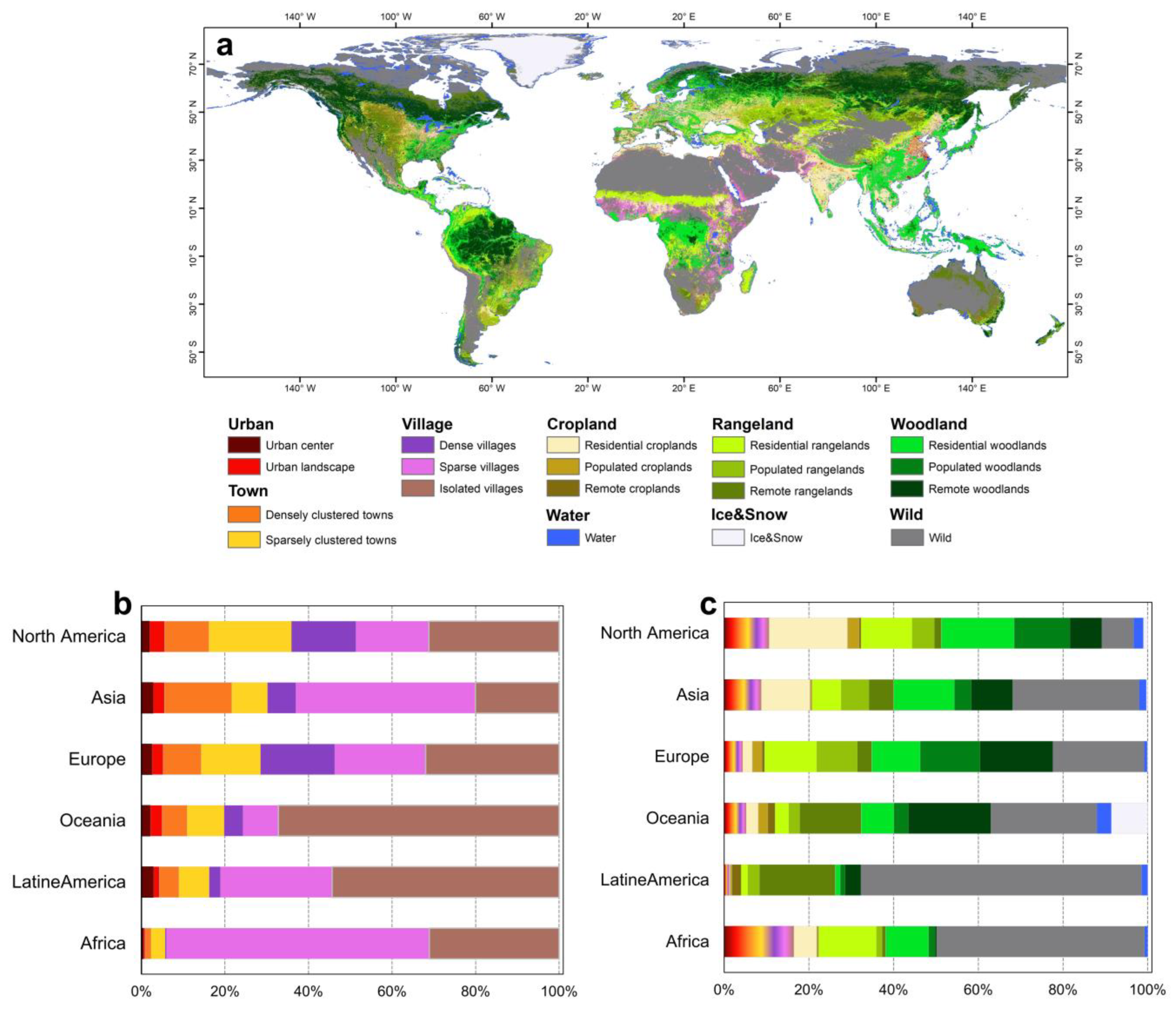
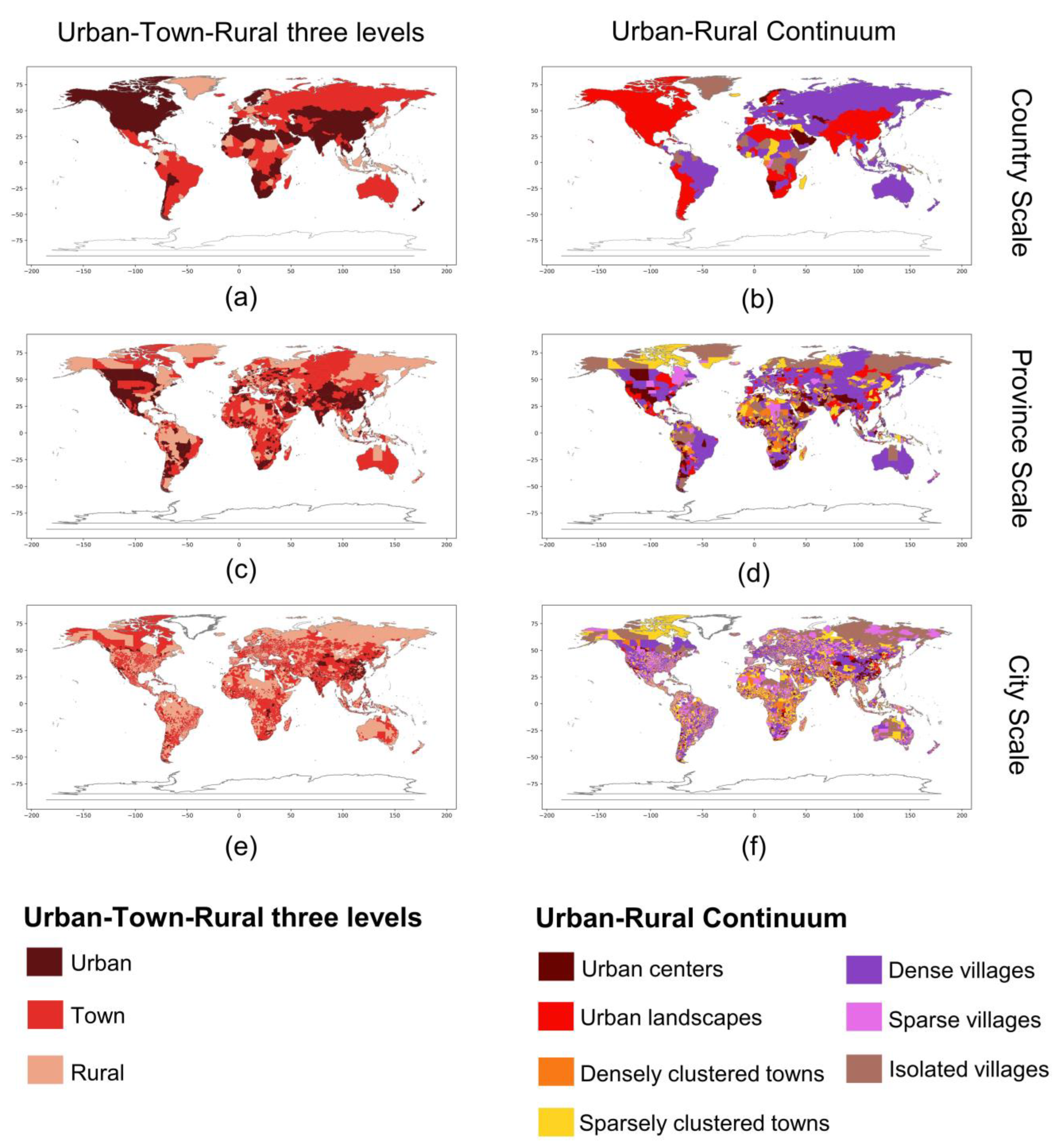
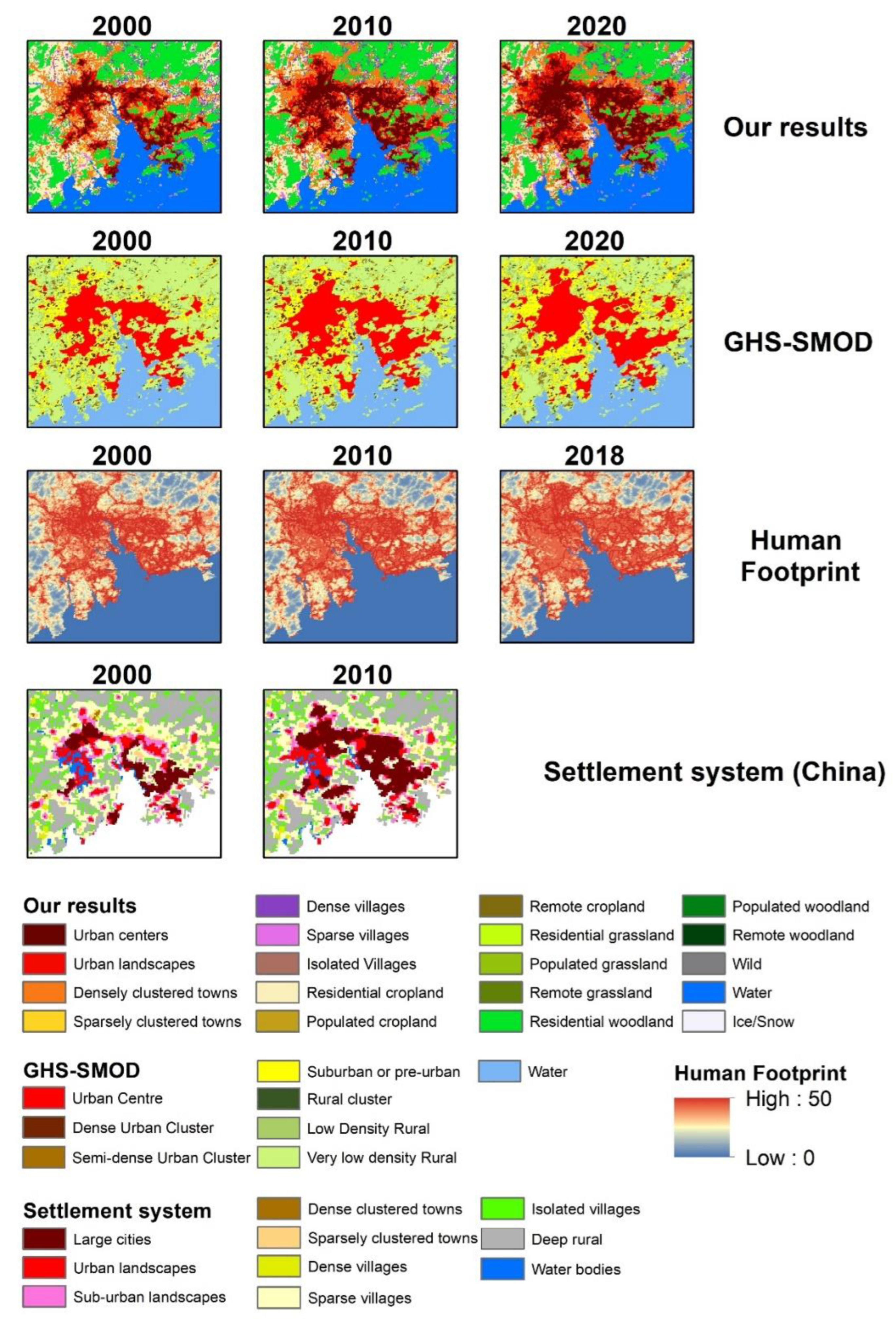
3.1. Global Human Settlement Mapping Results in the Rural–Urban Continuum

A global map of human settlements in 2020 is shown in Figure 2a. Combining population data to show the gradient distribution of human activity intensity, this map shows more detailed information than land-cover maps, which can help us better understand the relationship between human activity and land use, urbanization, and its regional differences (Figure 2a).

The distribution of human settlements varied greatly among continents. The only thing in common is that the proportion of the rural–urban continuum is very small, but the proportion of different types in the rural–urban continuum is also very different, which reflects the different levels of urbanization across continents. In 2020, North America, Asia, and Europe respectively had the highest proportions of urban areas and towns (nearly 30%), but in Oceania and Latin America, this ratio was less than 20%. About 10% of Africa is urban areas and towns, and over 60% of the rural–urban continuum is dominated by sparse villages (Figure 2b).

Every continent has its most prevalent human settlements. Africa is dominated by sparse villages. Asia has the highest proportion of densely clustered towns. The proportion of dense villages in Europe is extremely high. Oceania and Latin America have a high proportion of isolated villages. And the rural–urban continuum of North America is relatively evenly proportioned (Figure 2b).

The higher the level of urbanization, the higher the degree of development of the natural land system. In continents with high levels of urbanization, such as North America, Asia, and Europe, there are higher proportions of residential cropland, rangeland, and woodland. In contrast, the proportion of uninhabited lands is higher in Oceania, Latin America, and Africa. Remote rangeland and woodland are the main parts, rather than residential areas. Africa has a very high proportion of sparse villages, resulting in a high proportion of its rural–urban continuum. Actually, most of the sparse villages in Africa are developed and utilized on bare land, whose development and utilization levels are only comparable to that of residential cropland and rangeland in other continents (Figure 2c).

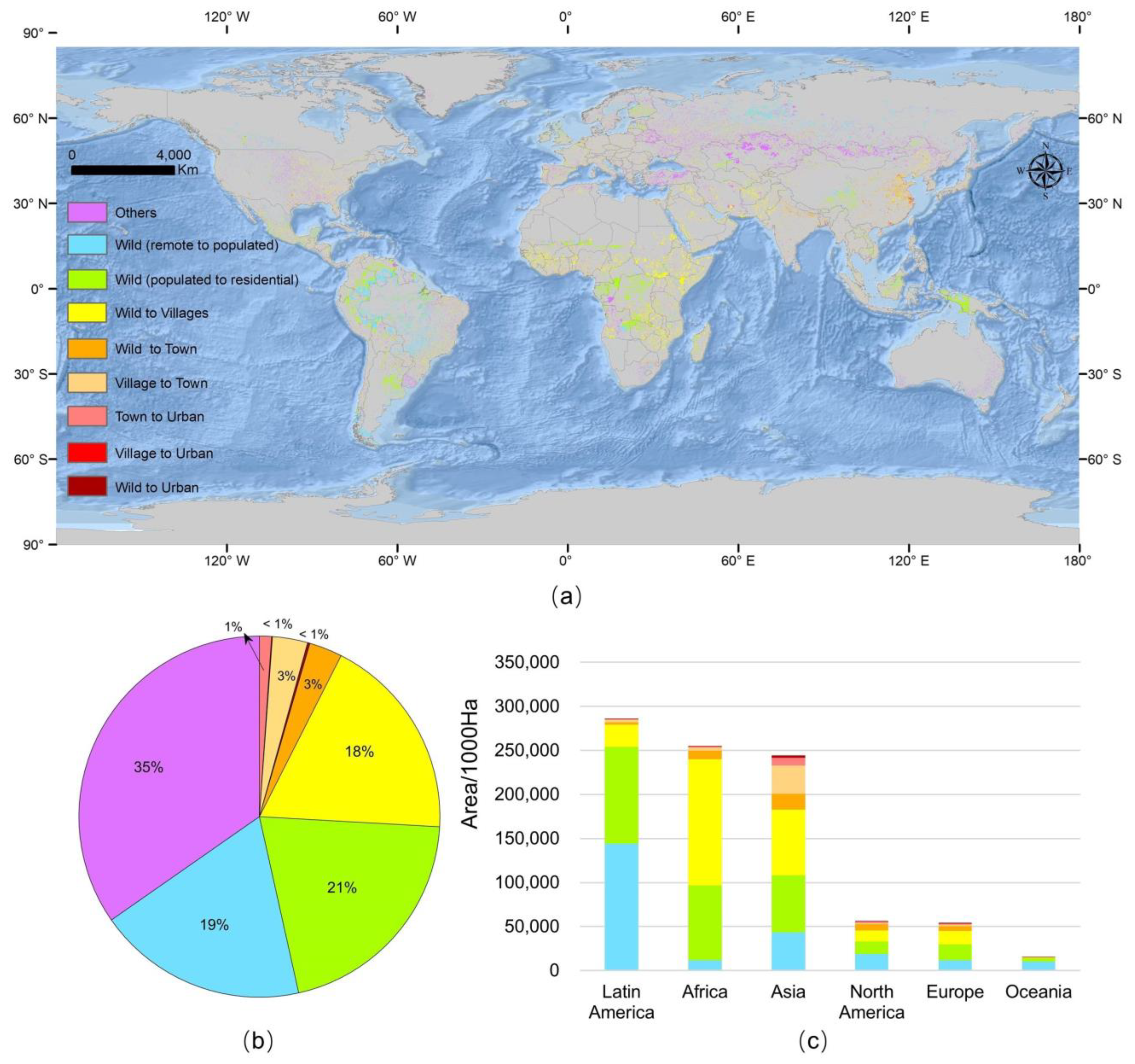
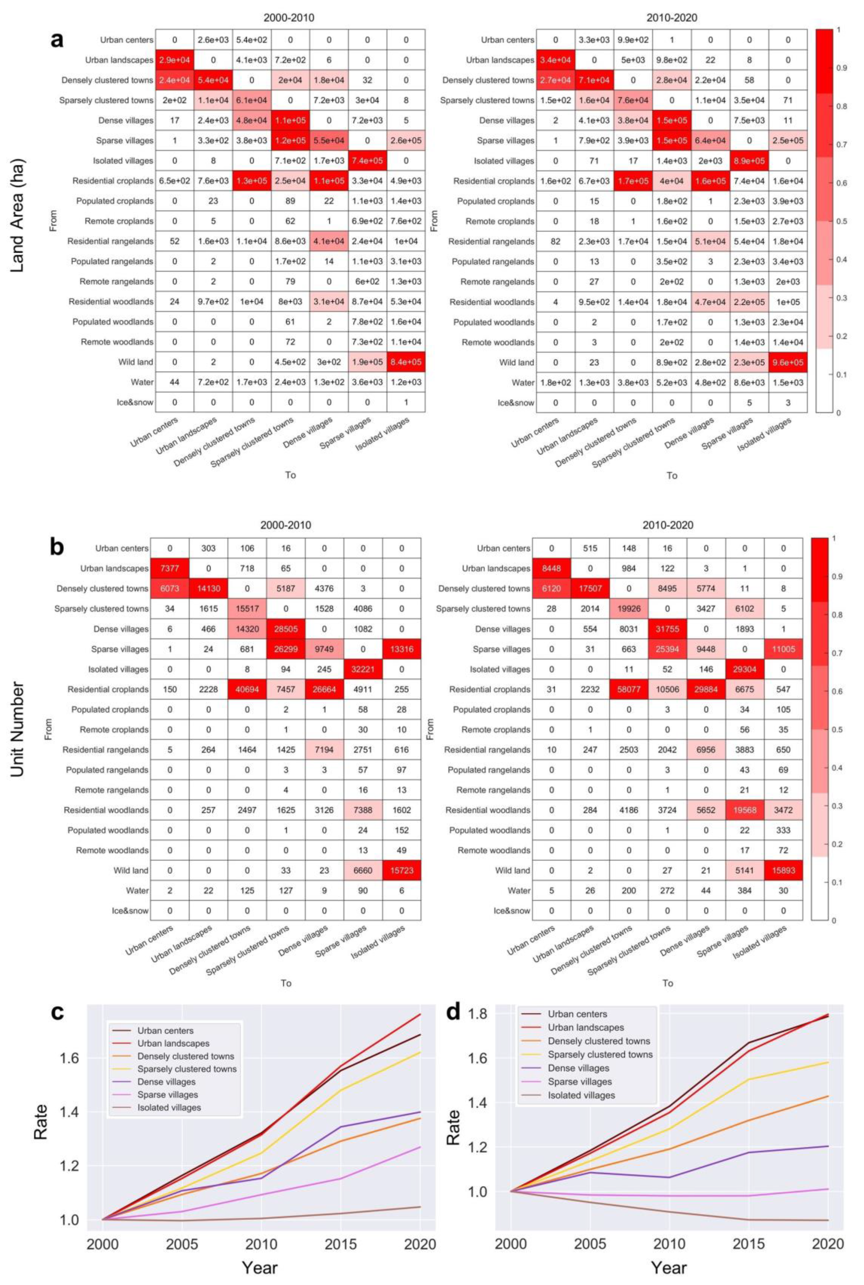
3.2. Global Human Settlement Change Trajectory in the Rural–Urban Continuum

Not only are there regional differences in the distribution status of various human settlements, but their change rates over the past two decades have also varied considerably. Urban areas in Africa and Asia have been developed exceeding or near the rate of 100%, while almost none of the human settlement types have been developed more than 50% in Oceania and Latin America (Figure 3a).

In general, urban areas have the highest growth rates in most regions except Europe and Latin America. More dense villages and sparsely clustered towns have been developed in Europe for the last two decades (Figure 3a), which indicates that the process of urbanization in Europe no longer needs to focus on the urban center but enriches the diverse peri-urban types in the rural–urban continuum. Dense villages are also the top growth type in Latin America, and they may take longer than two decades to develop into urban areas. The growth rate of sparsely clustered towns is the highest except for urban areas, which is consistent in each continent (Figure 3a). Sparse villages and isolated villages have expanded the least land area because this may only be the first station of long urbanization process over a period of 20 years. Further evidence will be found in an analysis of differences in the world continents’ human settlement change trajectory, which will provide an overall and detailed explanation for regional differences.

With the expansion of built-up areas and the increase in population, global human settlements are generally developing along a wild-rural–urban trajectory. In all of the changed global land, only about 35% became less affected by human activity (labeled as purple), which was mainly distributed in the north of the Eurasian continent (Figure 4a,b).

Globally, there were respectively 19%, 21%, and 18% of the changed global land completing the developing trajectory of wild (remote to populated), wild (populated to residential), wild to villages. Urbanization becomes more difficult and slows down when it comes to the developing stage of towns. Only less than 8% of the changed land developed into towns or urban areas. The origin of the town was about half cropland (mainly residential cropland) and half villages while urban areas almost completely came from towns (Figure 4b).

As vast and slowly developing continents, Latin America, Africa, and Asia were the top three continents with the largest change areas of land along the forward wild-rural–urban trajectory. Most of Africa’s wild area developed into villages over a 20-years interval while Latin America’s wildland recently became more intensely affected by human activities. Asia had the largest area of towns that developed from 2000 to 2020, especially towns developed from villages (Figure 4c).

From the perspective of the 10-year interval, there was a certain pattern of transformation among the types of human settlements. In general, the global human settlements followed the pattern that developed from wildland to villages (isolated—sparse—dense), and then to towns (sparse—dense), and finally to urban areas (edge—center) (Figure 5a,b).

More specifically, urban centers developed from the urban landscape and densely clustered towns. Densely clustered towns and dense villages originated from residential cropland mainly, while sparsely clustered towns used to be mainly dense villages and sparse villages. The future of isolated villages is sparse villages.

Urbanization was not only reflected in the expansion of the land area in the rural–urban continuum, but also in the phenomenon that the number of cities and towns increased while the number of villages decreased (Figure 5c,d). Over the past 20 years, all types of the rural–urban continuum have expanded in land area, but with different changes in quantity: the number of urban areas has increased by 80%, the number of towns has increased by between 40% and 60%, and the number of villages has increased slowly (20%), remained constant, or even decreased. These increased rural–urban continuum types were all converted from the natural land system in less than 20 years (Figure 5c,d).

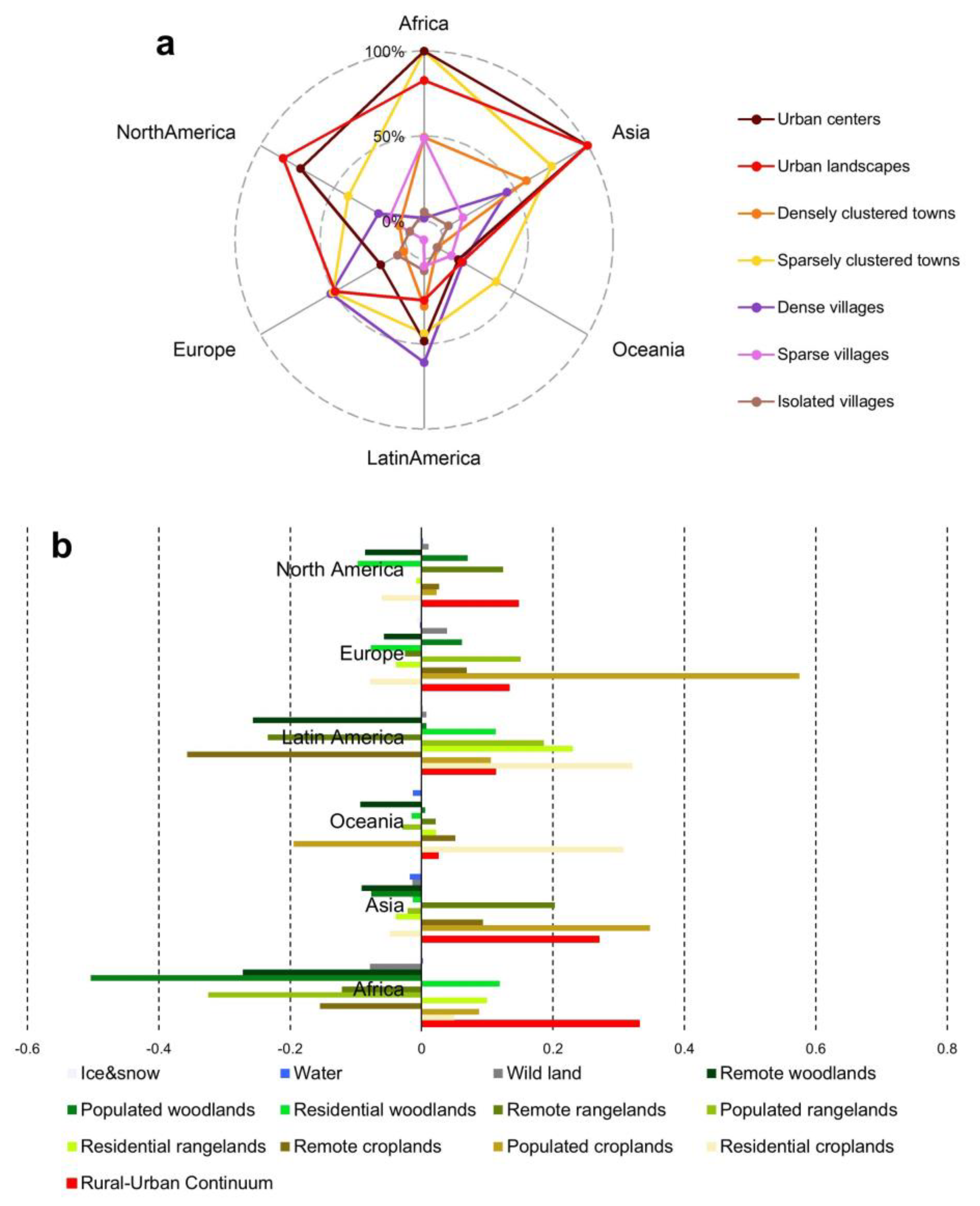
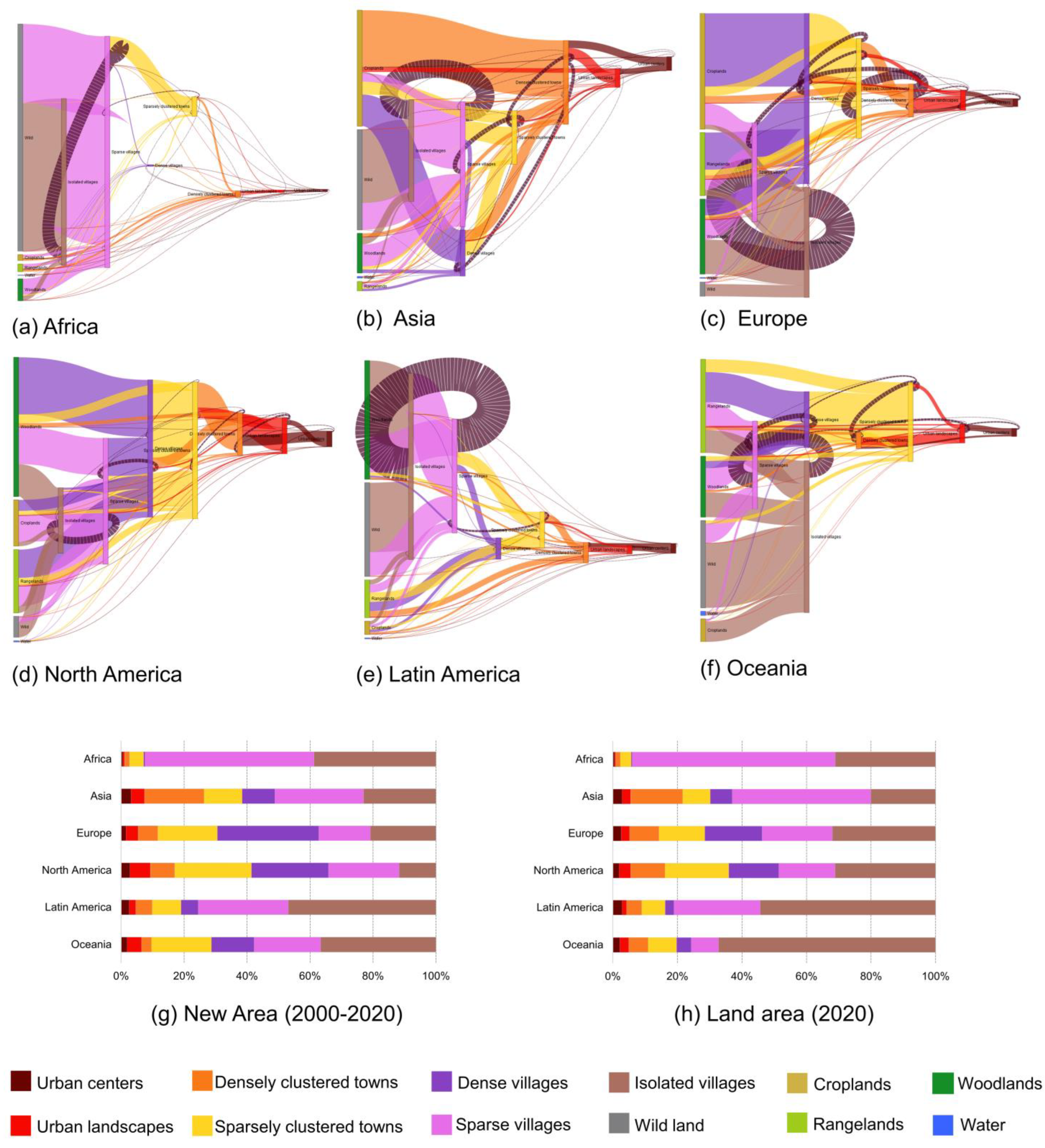
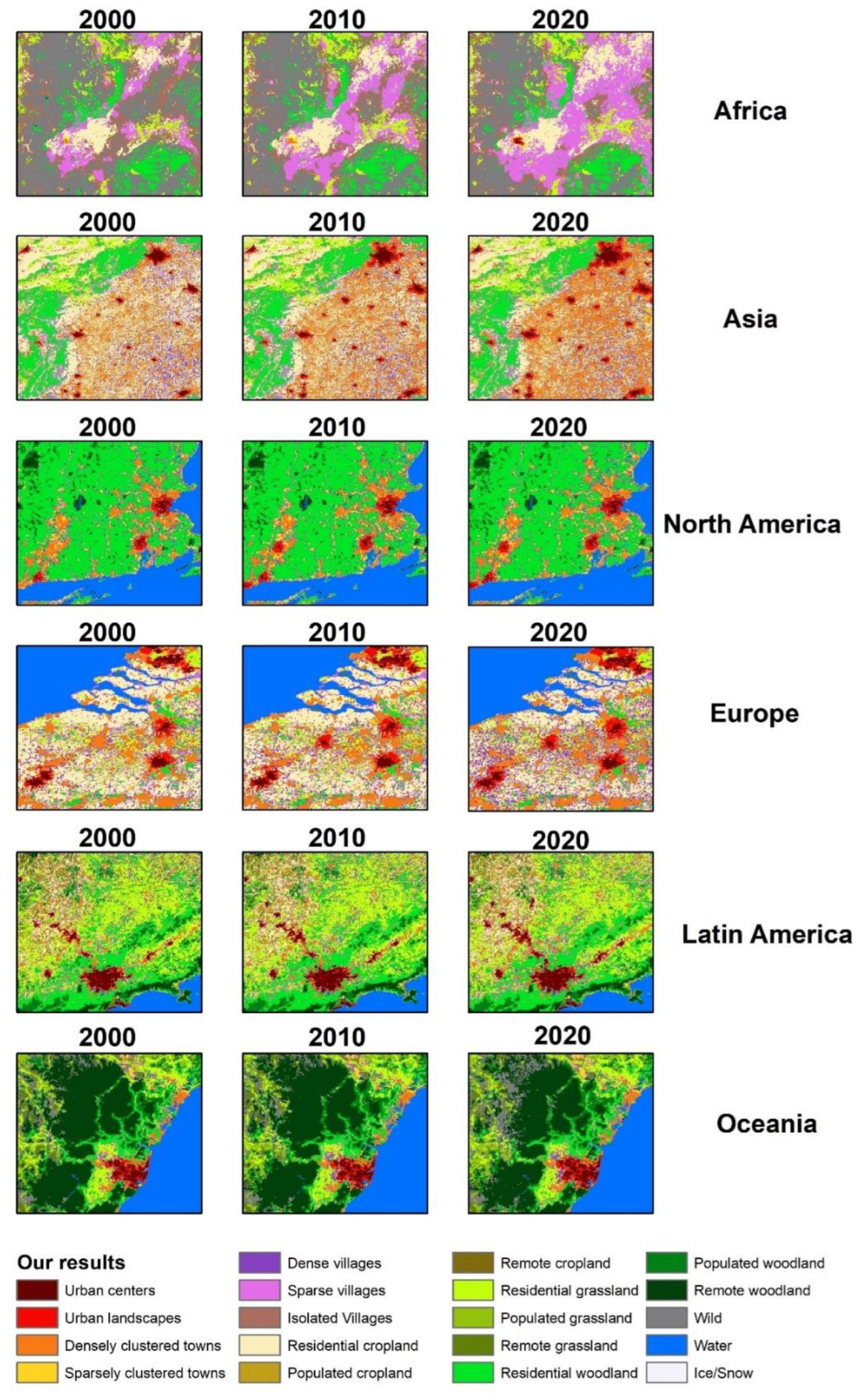
3.3. Continent-Scale Urbanization Characteristics

From a regional perspective, human settlements mainly followed the pattern that developed from wildland to villages (isolated—sparse—dense), then to towns (sparse—dense), and finally to urban areas (edge—center), but there were some obvious differences in the structural features of human settlement development progress: Africa is dominated by sparse villages; Asia has the highest proportion of dense clustered towns; the proportion of dense villages in Europe is extremely high; Oceania and Latin America have a high proportion of isolated villages; and the rural–urban continuum of North America is relatively evenly proportioned (Figure 6).

Not all types of human settlement in each continent followed established development patterns. Generally, sparse villages and not isolated villages were formed first in Europe and Oceania. Sparse villages and dense villages were formed in the second phase of Asia’s human settlement development progress parallelly not progressively. Only human settlements in three continents (North America, Latin America, Africa) followed established patterns, although there were still some great differences in their development progress. In Africa, the process of human settlement development is stuck at the stage of sparse villages. Very few from this stage continue to develop into dense villages or towns, let alone urban areas. This difficult situation is alleviated in Latin America, whereas in North America there is no such problem, where dense villages and sparsely clustered towns are the main stages in the development process (Figure 6).

There were also some differences in the source of the rural–urban continuum. Wildland was the main source of the rural–urban continuum in Africa; both cropland and wildland contributed to the formation of the rural–urban continuum in Asia; and as for North America, the greatest contribution came from woodland. Unlike in other continents, grassland was also a major contributor in Europe and Oceania (Figure 6).

Not all urbanization processes end in becoming an urban center. From the detailed mapping result, the patterns of urbanization in different regions were captured more intuitively. In Europe, a lot of dense villages emerged outside of urban areas or in transition zones between urban areas and towns. Densely clustered towns are the most common human settlements in Asia; they are usually developed from residential cropland and continue to expand the land area further rather than becoming urban areas with a greater density of built-up area and population. In Africa, sparse villages are the most easily developed human settlements type from natural land systems, but their urbanization process probably ends for this status (Figure 7).

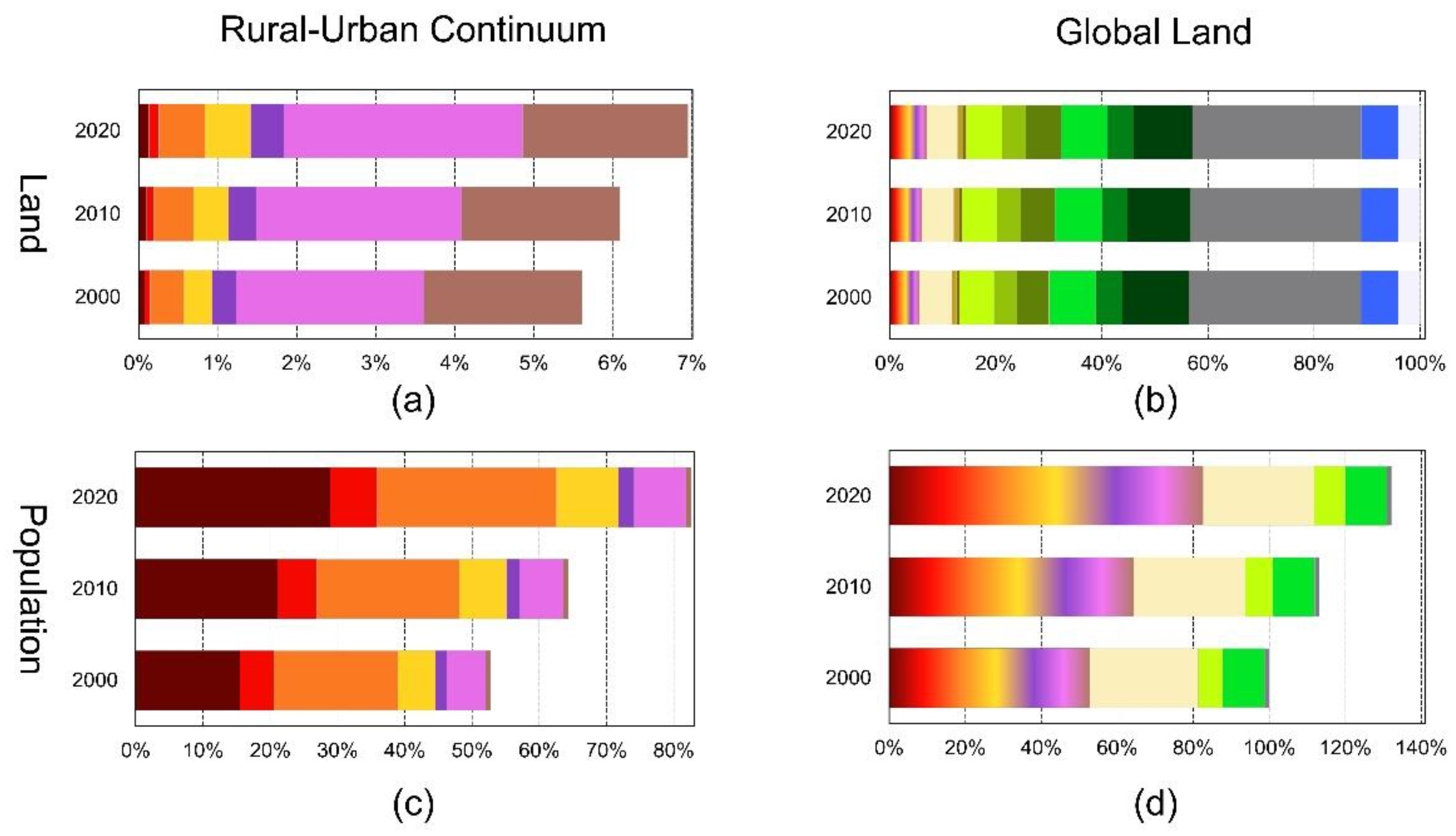
3.4. Land and Population in the Rural–Urban Continuum

Human activity reshapes the land surface unevenly. On the whole, the degree of reshaping increases step by step from wild, rural to urban, specifically manifested as the increase in population and land expansion (Figure 8). The rural–urban continuum is the most active part of all the global land, which only covers less than 7% of the global land area but its area has increased by 20% in the past two decades, while other land types have shown weak increases (<5%) or decreases. In addition to urban areas (increasing nearly 70%), the largest increase in the rural–urban continuum was also observed in sparsely clustered towns (~60%) (Figure 4c).

With the land-area expansion of the rural–urban continuum, more and more people live in the rural–urban continuum, especially in urban and peri-urban areas. In 2020, more than 60% of the world’s population lived on less than 7% of the land, and 86% of this population lived mainly in urban areas and towns (approximately 20% of the land area) (Figure 8a,c). In urban areas and towns, the growth rate of the land tends to increase every decade, and the growth rate of the population (30%) is even greater than that of the land (25%).

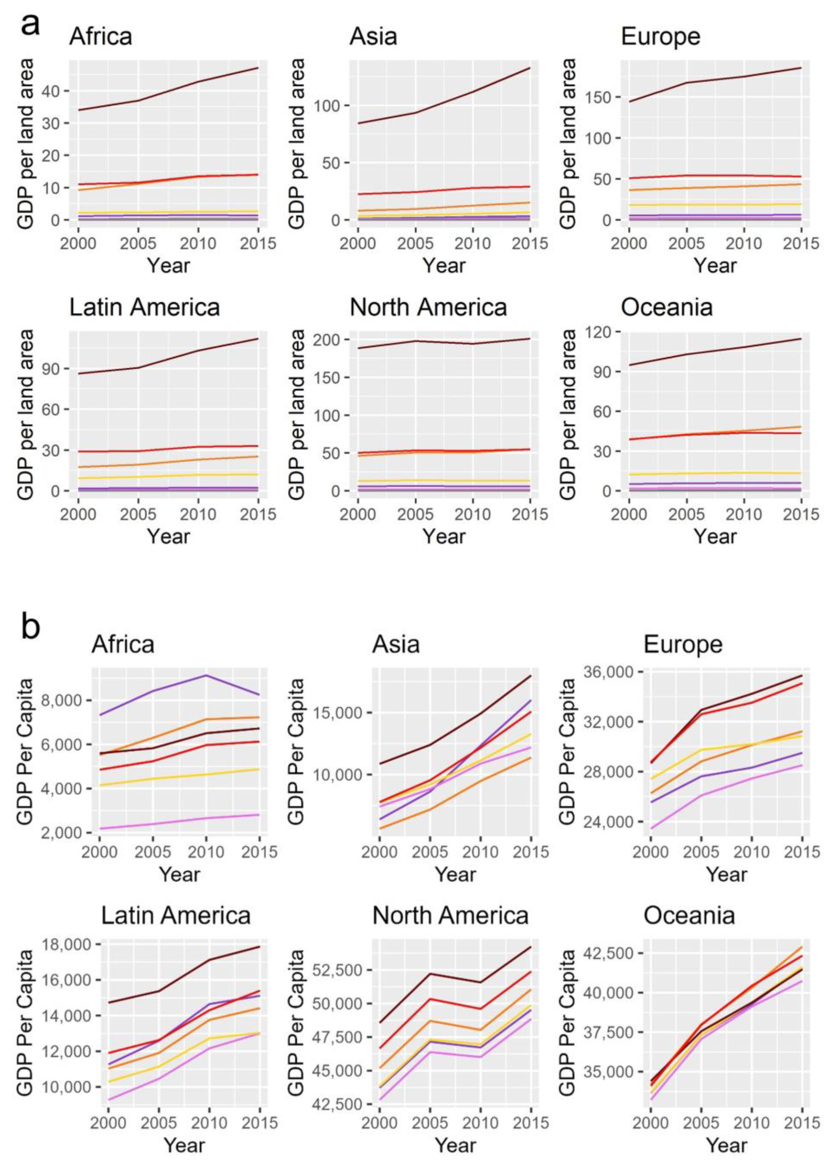
3.5. Economic Growth in Each Human Settlement

In our study, types in the rural–urban continuum are defined and divided using built-up density and population density. The type of rural–urban continuum reflects the combination of built-up density and population density at different levels, whose geographical differences are obvious. Economic factors are also important indicators that distinguish between urban and rural areas. It is worth exploring the role of various human settlement types in economic production, especially its differences in geography. Analysis of economic growth may also provide new insights into the different trajectories of urbanization in each continent.

GDP output per unit area of different human settlement is different. Generally, its value increases step by step along the rural–urban continuum, which is consistent across different continents. Urban centers have the highest production efficiency, while in second place are urban landscapes and densely clustered towns; they differ little in Africa, North America, and Oceania (Figure 9a). In rural areas, it is more difficult to convert land into economic value, which is consistent with our understanding of the intensity of talent and land needed for economic production. Although the relative difference in GDP among types in the rural–urban continuum per unit of land is consistent in all continents, the absolute amount of GDP per unit of land still differs a lot in all continents, which is related to the layout of the global industrial chain and international trade.

Unlike GDP per land area, the GDP per capita of different human settlements is more complex across world continents. Consistent with the evenly proportioned area of human settlements in its development process (Figure 6), the GDP per capita in North America also increases step by step along the rural–urban continuum. In Asia, Africa, and Latin America, which are mostly developing countries, the GDP per capita in dense villages is quite high. In Asia and Latin America, the GDP per capita in dense villages is near that of urban landscapes while the GDP per capita of dense villages is the highest in Africa. This phenomenon was not found in any other continent (Figure 9b). To some extent, this shows the importance of rural revitalization for developing countries. As for the inequality, in Oceania, the GDP per capita differs little in the rural–urban continuum, while Africa has the widest gap in GDP per capita in the rural–urban continuum; the GDP per capita in dense villages is nearly four times higher than in sparse villages (Figure 9b).

4. Discussion

4.1. Implications

The urbanization process is taking place in different and distinctive ways around the world. In our research, this difference in the urbanization process was viewed as the difference in the human settlement change trajectory, which was represented by the change in population and built-up area.

This provides new insights when looking at changes in human settlements from the perspective of the rural–urban continuum. There is only a small percentage of new land area expanded in urban areas, even in North America, the most urbanized region, at less than 10%. The vast majority of new built-up areas occur in rural landscapes like towns and villages. This conclusion was confirmed in other regional scale studies. Most of the built-up land in European countries is dominated by rural landscape [44], most of the built-up area expansion in South America occurs in small cities and around rural areas, not only concentrated around major cities [45]. And in China, the new built-up area is mostly concentrated in rural landscapes rather than big cities [17]. A rural revival is needed to counter urbanization around the globe [46]. As a key initial or intermediate stage in the process of urbanization, towns and villages need additional attention in the future for better coordination and balance between built-up areas, population, and economic growth.

Our study also provides insights into the differences in urbanization paths in different regions of the globe. Sun et al. found that large cities in the low-income and lower-middle-income countries had the highest urban population growth, and built-up area expansion in the upper-middle-income countries was more than three times that of the high-income countries [25]. Tian et al. found that the increases in population density and built-up patch density were the main characteristics of Asia and Africa [26]. Our results also indicated that the growth rate of urban areas in regions dominated by developing countries such as Asia and Africa was much higher than that of North America, Europe, and Oceania (Figure 3a). Tian et al. also found that urbanization in Europe and North America took a rather steady pace, combined with widespread greening [26]. This is consistent with our findings that the urbanization process in Europe over the past two decades has been dominated by the development of dense villages, indicating slower urbanization in Europe. A general trend of population decline in Europe since 2000 has been observed in recently published literature [47]. And the rural–urban continuum of North America is relatively evenly proportioned in the urbanization process (Figure 6).

There could be multiple drivers leading to differences in the urbanization path across the globe. Original land cover varies widely across continents, with more than half of human settlements in Asia and Europe originating in agricultural land systems, while the vast majority of human settlements in Africa have been developed from wild bare land (Figure 6). While there is no direct evidence of causal inference, it is likely that the original land system is related to the most prevalent human settlement types in the urbanization process. Economic development and urbanization complement each other. The population share living in metropolitan areas above 1 million is roughly four times higher in high-income (47%) than in low-income countries (12%). While urbanization does not necessarily lead to economic development, economic development does not happen without urbanization [9]. Aggregation of population and land (especially built-up area) can generate scale effects and boost economic development, thus obtaining the feedback of capital to support and promote the construction of real estate and infrastructure. As a result, economically developed countries can often enter a virtuous cycle of urbanization, as the example of North America shows (Figure 6). In addition, policy factors are also a very important part. Over last two decades, the Chinese government has developed many macro strategies in support of regional sustainable and coordinated development, including the China Western Development Plan (1999), Northeast Area Revitalization Plan (2004), and Rise of Central China Plan (2016) [30]. The trajectory of urbanization is deeply influenced by the management measures issued by the government. Policy in China has truly promoted the development of rural areas, which could be seen in the characteristic landscape of densely clustered towns distributed on the cropland plain (Figure 8).

The detailed mapping results of human settlements in this study can be used as analyzable raster images to meet the diversified needs of land-use data input in the future. A clear definition of the rural–urban continuum and pixel-level global maps provide a database for analyzing inequality in social welfare and infrastructure, including services [3], education, income [48], health care [49], and green space [25,26].

4.2. Scale Effects of Human Settlement Development Progress

In this section, we identified the development stages with the largest proportion of land-area growth at three geographic scales. We found that with the geographic scale becoming increasingly deeper, the unified characteristics of the continents were further diluted, and the different characteristics of the local areas appeared (Figure 10).

At country scale, countries with the largest increases in urban area are spread across all continents. Contrary to the observed characteristics of the continents, there are also some African countries with the largest proportion of urban area growth, but Africa is the continent with the largest differences among countries, for there are also some countries stuck in the stage of town and rural development (Figure 10a,b).

It is worth noting that in such a multiscale analysis, geographical units grouped into the same category according to the development process of human settlements may have completely different levels of economic development. For example, in the United States and some third world countries, there is the highest growth rate in urban areas. However, from the overall analysis on the continental scale in Section 3.3, it can be seen that the original urban area of North America is large, and all types of human settlements develop in a balanced and coordinated way, while countries in Africa that originally had a very low level of urbanization have just entered the period of rapid development in the past two decades.

By the same token, the reasons behind some geographical units that are also classified as rural are quite different. For example, in some areas of Europe, urbanization is almost complete, so they can only focus on rural development at this stage. However, some countries in Asia, Africa, and Latin America are still in the early stage of urbanization, trying to revitalize the countryside.

4.3. Uncertainties and Limitations

The criteria and thresholds for the division of urban and rural areas have always been difficult to determine and are different across countries worldwide. Therefore, it is very meaningful to propose a classification system of the global rural–urban continuum and produce the mapping result, so that we can compare the differences in the urbanization process on a global scale. Inevitably, some local specificities have been overlooked in this global effort. So, we compared the spatial distribution of our data products with other similar human settlement mapping products (Figure 11). Although different classification systems are not completely the same, it can be seen from the results that the data products in this study have a strong consistency with other data products in spatial distribution, which can reflect the continuous changes in urban expansion in a long time series. In addition, it also provides finer details of the urbanization progress in the rural–urban continuum.

The differences in human settlement types in the rural–urban continuum are mainly represented by the difference in population density and built-up area density. Based on the World Cities Database, which includes almost all populated places in the world (about 4.3 million), we validated the mapping results by two factors (population density and built-up area density). Results showed that the classification system adopted in this study can effectively reflect the difference in the continuous levels between population density and built-up area density in the rural–urban continuum (Figure 12).

However, there are still some deficiencies in terms of data and methods. In terms of data, the population data used in this study decomposed census-based count results into grid cells using machine learning methods, in which a certain amount of the population was decomposed into cropland, grassland, and woodland, which did not completely correspond to the built-up area data layer, although this information provided us with an understanding of the level of human activities in natural land systems. Similarly, in land-cover data, there is also the problem of poor identification of built-up areas in natural land systems. To solve this problem, except for the main mapping process, we post-processed the grid whose population density met the corresponding conditions while the built-up density did not. Since the research was carried out on a scale of 1 km, there may be bias in the numerical estimation of the land area due to the coarse resolution.

As for the method, corresponding to the threshold problem, the formulation of the classification system also ignores the particularity of the local landscape. This study only considered the two factors (population and built-up area) in the process of mapping the rural–urban continuum. In Section 4.3, it was also mentioned that the economic factor is also the main difference between urban and rural areas. In addition, the urban–rural differences in human welfare such as in income, education, and health are also worth exploring. The simple decision tree classification system in this study can be applied in the Google Earth Engine to efficiently produce mapping products. However, the complex differences between urban and rural areas around the world still need to be deeply and carefully excavated.

5. Conclusions

From the perspective of the rural–urban continuum, urban and rural areas are two poles of a gradient with many continuous human settlements in between. Using global land-cover data (FROM-GLC Plus) and global population data (Worldpop) based on the decision tree method, this study proposed a method and classification system for global rural–urban continuum mapping and produced the mapping results on a global scale in the Google Earth Engine platform.

Our results indicated that global human settlements follow the pattern that develops from wildland to villages (isolated—sparse—dense), then to towns (sparse—dense), and finally to urban areas (edge—center). Over the past 20 years, all types of cities, towns, and villages have expanded in land area but with different trends in quantity; contrasted with the dramatic growth of urban areas (80%) and towns (40–60%), the number of villages has increased slowly (20%) or even decreased. From a regional perspective, North America, Asia, and Europe respectively had the highest proportions of urban areas and towns (nearly 30%) in the rural–urban continuum, but in Oceania and Latin America, this ratio was less than 20%. Urban areas and towns in Africa comprise only about 10%. There are also some obvious differences in the structural features of urbanization progress: Africa is dominated by sparse villages; Asia has the highest proportion of densely clustered towns; the proportion of dense villages in Europe is extremely high; Oceania and Latin America have a high proportion of isolated villages; and the rural–urban continuum of North America is relatively evenly proportioned. Rural–urban continuum mapping and analysis provide a database and new insights into urbanization and the differences between urban and rural areas around the world.

References

1. Ellis, E.C.; Beusen, A.H.W.; Goldewijk, K.K. Anthropogenic Biomes: 10,000 BCE to 2015 CE. Land 2020, 9, 129. [Google Scholar] [CrossRef]
2. Ellis Erle, C.; Kaplan Jed, O.; Fuller Dorian, Q.; Vavrus, S.; Klein Goldewijk, K.; Verburg Peter, H. Used planet: A global history. Proc. Natl. Acad. Sci. USA 2013, 110, 7978–7985. [Google Scholar] [CrossRef] [PubMed]
3. Cattaneo, A.; Nelson, A.; McMenomy, T. Global mapping of urban–rural catchment areas reveals unequal access to services. Proc. Natl. Acad. Sci. USA 2021, 118, e2011990118. [Google Scholar] [CrossRef]
4. van Vliet, J.; Birch-Thomsen, T.; Gallardo, M.; Hemerijckx, L.-M.; Hersperger, A.M.; Li, M.; Tumwesigye, S.; Twongyirwe, R.; van Rompaey, A. Bridging the rural-urban dichotomy in land use science. J. Land Use Sci. 2020, 15, 585–591. [Google Scholar] [CrossRef]
5. Lang, R.E.; Dhavale, D. Beyond Megalopolis: Exploring America’s New “Megapolitan” Geography; Brookings Mountain West: Las Vegas, NV, USA, 2005; pp. 1–33. [Google Scholar]
6. Alexander Wandl, D.I.; Nadin, V.; Zonneveld, W.; Rooij, R. Beyond urban–rural classifications: Characterising and mapping territories-in-between across Europe. Landsc. Urban Plan. 2014, 130, 50–63. [Google Scholar] [CrossRef]
7. Cyriac, S.; Firoz, C.M. Dichotomous classification and implications in spatial planning: A case of the Rural-Urban Continuum settlements of Kerala, India. Land Use Policy 2022, 114, 105992. [Google Scholar] [CrossRef]
8. Shaw, B.J.; van Vliet, J.; Verburg, P.H. The peri-urbanization of Europe: A systematic review of a multifaceted process. Landsc. Urban Plan. 2020, 196, 103733. [Google Scholar] [CrossRef]
9. OECD & European Commission. Cities in the World: A New Perspective on Urbanisation. 2020. Available online: https://www.oecd.org/publications/cities-in-the-world-d0efcbda-en.htm (accessed on 13 August 2023).
10. Benet, F. Sociology Uncertain: The Ideology of the Rural-Urban Continuum. Comp. Stud. Soc. Hist. 1963, 6, 1–23. [Google Scholar] [CrossRef]
11. Dewey, R. The Rural-Urban Continuum: Real but Relatively Unimportant. Am. J. Sociol. 1960, 66, 60–66. [Google Scholar] [CrossRef]
12. Pahl, R.E. THE RURAL-URBAN CONTINUUM1. Sociol. Rural. 1966, 6, 299–329. [Google Scholar] [CrossRef]
13. Sorokin, P.A.; Zimmerman, C.C. Principles of Rural-Urban Sociology; Henry Holt: New York, NY, USA, 1929. [Google Scholar]
14. Wirth, L. Urbanism as a Way of Life. Am. J. Sociol. 1938, 44, 1–24. [Google Scholar] [CrossRef] [Green Version]
15. Hines, F.K.; Brown, D.L.; Zimmer, J.M. Social and Economic Characteristics of the Population in Metro and Nonmetro Counties, 1970; Economic Research Service, US Department of Agriculture: Washington, DC, USA, 1975.
16. Yang, X.; Wang, Q.; Zhou, Q. Regional habitat units in the context of urban-rural China: Concept, mechanism and features. Habitat Int. 2022, 128, 102668. [Google Scholar] [CrossRef]
17. Li, M.; van Vliet, J.; Ke, X.; Verburg, P.H. Mapping settlement systems in China and their change trajectories between 1990 and 2010. Habitat Int. 2019, 94, 102069. [Google Scholar] [CrossRef]
18. Dijkstra, L.; Florczyk, A.J.; Freire, S.; Kemper, T.; Melchiorri, M.; Pesaresi, M.; Schiavina, M. Applying the Degree of Urbanisation to the globe: A new harmonised definition reveals a different picture of global urbanisation. J. Urban Econ. 2021, 125, 103312. [Google Scholar] [CrossRef]
19. Schiavina, M.; Melchiorri, M.; Pesaresi, M.; Politis, P.; Freire, S.; Maffenini, L.; Florio, P.; Ehrlich, D.; Goch, K.; Tommasi, P. GHSL Data Package 2022; Publications Office of the European Union: Luxembourg, 2022. [Google Scholar]
20. van Vliet, J.; Eitelberg, D.A.; Verburg, P.H. A global analysis of land take in cropland areas and production displacement from urbanization. Glob. Environ. Change 2017, 43, 107–115. [Google Scholar] [CrossRef]
21. UN Habitat. The Strategic Plan 2020–2023. 2019. Available online: https://unhabitat.org/the-strategic-plan-2020-2023 (accessed on 13 August 2023).
22. Gong, P.; Li, X.; Wang, J.; Bai, Y.; Chen, B.; Hu, T.; Liu, X.; Xu, B.; Yang, J.; Zhang, W.; et al. Annual maps of global artificial impervious area (GAIA) between 1985 and 2018. Remote Sens. Environ. 2020, 236, 111510. [Google Scholar] [CrossRef]
23. Liu, X.; Huang, Y.; Xu, X.; Li, X.; Li, X.; Ciais, P.; Lin, P.; Gong, K.; Ziegler, A.D.; Chen, A.; et al. High-spatiotemporal-resolution mapping of global urban change from 1985 to 2015. Nat. Sustain. 2020, 3, 564–570. [Google Scholar] [CrossRef]
24. Schmitt, A.; Uth, P.; Standfuß, I.; Heider, B.; Siedentop, S.; Taubenböck, H. Quantitative assessment and comparison of urban patterns in Germany and the United States. Comput. Environ. Urban Syst. 2023, 100, 101920. [Google Scholar] [CrossRef]
25. Sun, L.; Chen, J.; Li, Q.; Huang, D. Dramatic uneven urbanization of large cities throughout the world in recent decades. Nat. Commun. 2020, 11, 5366. [Google Scholar] [CrossRef]
26. Tian, Y.; Tsendbazar, N.-E.; van Leeuwen, E.; Fensholt, R.; Herold, M. A global analysis of multifaceted urbanization patterns using Earth Observation data from 1975 to 2015. Landsc. Urban Plan. 2022, 219, 104316. [Google Scholar] [CrossRef]
27. Di Marco, M.; Venter, O.; Possingham, H.P.; Watson, J.E.M. Changes in human footprint drive changes in species extinction risk. Nat. Commun. 2018, 9, 4621. [Google Scholar] [CrossRef] [PubMed] [Green Version]
28. Pecl Gretta, T.; Araújo Miguel, B.; Bell Johann, D.; Blanchard, J.; Bonebrake Timothy, C.; Chen, I.C.; Clark Timothy, D.; Colwell Robert, K.; Danielsen, F.; Evengård, B.; et al. Biodiversity redistribution under climate change: Impacts on ecosystems and human well-being. Science 2017, 355, eaai9214. [Google Scholar] [CrossRef]
29. Cumming, G.S.; Buerkert, A.; Hoffmann, E.M.; Schlecht, E.; von Cramon-Taubadel, S.; Tscharntke, T. Implications of agricultural transitions and urbanization for ecosystem services. Nature 2014, 515, 50–57. [Google Scholar] [CrossRef] [PubMed]
30. Jiang, H.; Sun, Z.; Guo, H.; Weng, Q.; Du, W.; Xing, Q.; Cai, G. An assessment of urbanization sustainability in China between 1990 and 2015 using land use efficiency indicators. npj Urban Sustain. 2021, 1, 34. [Google Scholar] [CrossRef]
31. Li, X.; Gong, P. Urban growth models: Progress and perspective. Sci. Bull. 2016, 61, 1637–1650. [Google Scholar] [CrossRef]
32. European, C.; Joint Research, C.; Freire, S.; Corbane, C.; Zanchetta, L.; Schiavina, M.; Politis, P.; Kemper, T.; Ehrlich, D.; Pesaresi, M.; et al. GHSL Data Package 2019: Public Release GHS P2019; Publications Office: Luxembourg, 2019. [Google Scholar]
33. Balk, D.; Montgomery, M.R.; Engin, H.; Lin, N.; Major, E.; Jones, B. Urbanization in India: Population and Urban Classification Grids for 2011. Data 2019, 4, 35. [Google Scholar] [CrossRef] [PubMed]
34. Jin, X.; Long, Y.; Sun, W.; Lu, Y.; Yang, X.; Tang, J. Evaluating cities’ vitality and identifying ghost cities in China with emerging geographical data. Cities 2017, 63, 98–109. [Google Scholar] [CrossRef]
35. Sun, H.; Liu, Y.; Xu, K. Hollow villages and rural restructuring in major rural regions of China: A case study of Yucheng City, Shandong Province. Chin. Geogr. Sci. 2011, 21, 354–363. [Google Scholar] [CrossRef]
36. Mu, H.; Li, X.; Wen, Y.; Huang, J.; Du, P.; Su, W.; Miao, S.; Geng, M. A global record of annual terrestrial Human Footprint dataset from 2000 to 2018. Sci. Data 2022, 9, 176. [Google Scholar] [CrossRef]
37. Yu, L.; Du, Z.; Dong, R.; Zheng, J.; Tu, Y.; Chen, X.; Hao, P.; Zhong, B.; Peng, D.; Zhao, J.; et al. FROM-GLC Plus: Toward near real-time and multi-resolution land cover mapping. GIScience Remote Sens. 2022, 59, 1026–1047. [Google Scholar] [CrossRef]
38. Tatem, A.J. WorldPop, open data for spatial demography. Sci. Data 2017, 4, 170004. [Google Scholar] [CrossRef] [PubMed]
39. Farr, T.G.; Rosen, P.A.; Caro, E.; Crippen, R.; Duren, R.; Hensley, S.; Kobrick, M.; Paller, M.; Rodriguez, E.; Roth, L.; et al. The Shuttle Radar Topography Mission. Rev. Geophys. 2007, 45. [Google Scholar] [CrossRef] [Green Version]
40. Kummu, M.; Taka, M.; Guillaume, J.H.A. Gridded global datasets for Gross Domestic Product and Human Development Index over 1990–2015. Sci. Data 2018, 5, 180004. [Google Scholar] [CrossRef] [PubMed] [Green Version]
41. Runfola, D.; Anderson, A.; Baier, H.; Crittenden, M.; Dowker, E.; Fuhrig, S.; Goodman, S.; Grimsley, G.; Layko, R.; Melville, G.; et al. geoBoundaries: A global database of political administrative boundaries. PLoS ONE 2020, 15, e0231866. [Google Scholar] [CrossRef] [PubMed] [Green Version]
42. Safanelli, J.L.; Poppiel, R.R.; Ruiz, L.F.; Bonfatti, B.R.; Mello, F.A.; Rizzo, R.; Demattê, J.A.M. Terrain Analysis in Google Earth Engine: A Method Adapted for High-Performance Global-Scale Analysis. ISPRS Int. J. Geo-Inf. 2020, 9, 400. [Google Scholar] [CrossRef]
43. Cao, Y.; Carver, S.; Yang, R. Mapping wilderness in China: Comparing and integrating Boolean and WLC approaches. Landsc. Urban Plan. 2019, 192, 103636. [Google Scholar] [CrossRef]
44. van Vliet, J.; Verburg, P.H.; Grădinaru, S.R.; Hersperger, A.M. Beyond the urban-rural dichotomy: Towards a more nuanced analysis of changes in built-up land. Comput. Environ. Urban Syst. 2019, 74, 41–49. [Google Scholar] [CrossRef]
45. Andrade-Núñez, M.J.; Aide, T.M. Built-up expansion between 2001 and 2011 in South America continues well beyond the cities. Environ. Res. Lett. 2018, 13, 084006. [Google Scholar] [CrossRef]
46. Liu, Y.; Li, Y. Revitalize the world’s countryside. Nature 2017, 548, 275–277. [Google Scholar] [CrossRef] [Green Version]
47. Newsham, N.; Rowe, F. Understanding trajectories of population decline across rural and urban Europe: A sequence analysis. Popul. Space Place 2023, 29, e2630. [Google Scholar] [CrossRef]
48. Thiede, B.C.; Butler, J.L.W.; Brown, D.L.; Jensen, L. Income Inequality across the Rural-Urban Continuum in the United States, 1970–2016. Rural. Sociol. 2020, 85, 899–937. [Google Scholar] [CrossRef]
49. Sibley, L.M.; Weiner, J.P. An evaluation of access to health care services along the rural-urban continuum in Canada. BMC Health Serv. Res. 2011, 11, 20. [Google Scholar] [CrossRef]
Figure 1. Human settlement type mapping workflow.
Land 12 01607 g001
Figure 2. Distribution of global human settlements in 2020. (a) Mapping results of human settlements (2020). (b) Percentage of land area in 2020 occupied by each human settlement type of the rural–urban continuum in each continent. (c) Percentage of land area in 2020 occupied by each human settlement type of global land in each continent.
Land 12 01607 g002
Figure 3. Change rate of land area in human settlements by each continent from 2000 to 2020. (a) Each continent’s change rate for human settlements in the rural–wild continuum from 2000 to 2020. (b) Each continent’s change rate for human settlements in global land from 2000 to 2020.
Land 12 01607 g003
Figure 4. Distribution of human settlement change types (2000–2020). (a) Mapping results of human settlement change types (2000–2020). Wild refers to the types of human settlements outside of the rural–urban continuum (urban, town, and village). (b) Percentage of land area occupied by each human settlement change type. (c) Land area of each human settlement change type in each continent (except other change type, which refers to backward flow against wild-rural–urban direction).
Land 12 01607 g004
Figure 5. Change between human settlement types. (a) Land-area change matrixes of human settlements (ha, 2000–2010, 2010–2020). (b) Unit number change matrixes of human settlements (2000–2010, 2010–2020). The color of each cell represents the ratio of the value of the cell divided by the maximum value of the column in which the cell resides. (c) Land-area change rate of rural–urban settlements (2000–2020). (d) Unit number change rate of rural–urban settlements (2000–2020).
Land 12 01607 g005
Figure 6. Sankey maps of human settlement development progress (2000–2020, (a): Africa, (b): Asia, (c): Europe, (d): North America, (e): Latin America, (f): Oceania) and percentages of new areas ((g), during 2000–2020) and percentages of areas in 2020 (h) occupied by each human settlement type in each continent.
Land 12 01607 g006
Figure 7. Detailed mapping result of human settlements change trajectory.
Land 12 01607 g007
Figure 8. Land occupied by and population distributed in each type of human settlement. (a) Percentage of area occupied by each human settlement type in the rural–urban continuum. (b) Percentage of area occupied by each land type globally. (c) Percentage of population distributed in each human settlement type of the rural–urban continuum. (d) Percentage of population distributed in each land type globally. Percentage of population is calculated based on world total population in 2000.
Land 12 01607 g008
Figure 9. GDP growth in each human settlement from 2000 to 2015. (a) GDP per land area (USD/square meter) in each human settlement from 2000 to 2015. (b) GDP per capita (USD per capita) in each human settlement from 2000 to 2015. Legend is the same as Figure 5c,d.
Land 12 01607 g009
Figure 10. The largest percentage of increasing human settlement identified in the progress of urbanization at country scale (a,b), at province scale (c,d), at city scale (e,f) in the urban-town-rural three levels (a,c,e) and in the urban–rural continuum (b,d,f).
Land 12 01607 g010
Figure 11. Comparing our dataset with other related datasets.
Land 12 01607 g011
Figure 12. Population density and built-up density (ABDI, Adjusted Built-up Density Index) of human settlements samples in the rural–urban continuum. (a) Scatter plot of ABDI against the population density. (b) Distribution of population density in the rural–urban continuum. (c) Sample counts of different ABDI levels in the rural–urban continuum.
Land 12 01607 g012