Article

Cumulative Spatial and Temporal Analysis of Anthropogenic Impacts in the Protected Area of the Gran Paradiso National Park in the NW Alps, Italy

by
Chiara Richiardi
1,2,
Maria Rita Minciardi
3,
Consolata Siniscalco
2 and
Maria Adamo
1,*
1
National Research Council (CNR), Institute of Atmospheric Pollution Research (IIA), c/o Interateneo Physics Department, Via Amendola 173, 70126 Bari, Italy
2
Department of Life Sciences and Systems Biology, University of Torino, Via Pier Andrea Mattioli 25, 10125 Turin, Italy
3
Biodiversity and Ecosystem Services Laboratory, ENEA, Via Antica per Crescentino, 41, 13040 Saluggia, Italy
*
Author to whom correspondence should be addressed.
Land 2023, 12(6), 1124; https://doi.org/10.3390/land12061124
Submission received: 22 April 2023 / Revised: 23 May 2023 / Accepted: 23 May 2023 / Published: 24 May 2023
(This article belongs to the Special Issue Geospatial Data in Landscape Ecology and Biodiversity Conservation)

Abstract

:
Anthropogenic threats are responsible for habitat degradation and biodiversity decline. The mapping of the distribution and intensity of threats to biodiversity can be useful for informing efficient planning in protected areas. In this study, we propose a cumulative spatial and temporal analysis of anthropogenic impacts insisting on an alpine protected area, the Gran Paradiso National Park. The applied methodology starts with the construction of a spatial and temporal dataset of anthropogenic impacts and normalization based on relative intensity. The impacts analyzed include overgrazing, helicopter flights, road networks, built-up areas, worksites, derivations and discharges, sports activities, and dams and hydroelectric power plants. Each impact was assigned a weight based on its temporal persistence. Threats maps obtained from the collected, normalized, and weighted geodata are thus obtained. Finally, the risk map is calculated by combining the impact map with the vulnerability map, estimated through the methodology outlined in the Green Guidelines of the Metropolitan City of Turin. The risk map obtained was cross-referenced with the Park’s cartography to highlight any critical issues to specific habitats. Results show that most of the territory falls in low-risk (63%) or no-risk (35%) areas. However, there are some habitats that are totally or nearly totally affected by some degree of risk, although different to zero, such as the “Lentic waters with aquatic vegetation [incl. cod. 3130]”, the “Lentic waters partially buried”, the “Mountain pine forests (Pinus uncinata) [cod. 9430]”, and the “Mixed hygrophilous woods of broad-leaved trees [incl. cod. 91E0]”. This study highlights both the potential of these analyses, which enable informed management and planning of the fruition of protected areas, and the limitations of such approaches, which require in-depth knowledge of the territory and ecosystems and how they respond to threats in order to refine the model and obtain realistic maps.

1. Introduction

The landscapes of the Alps are strongly shaped by geomorphological complexity that deeply changes from the bottom of the valleys up to the rocky walls and the peaks determining different soil structures and profiles [1,2,3].
The history of human land use in the Alps testifies to the adaptability of humans to the harsh geomorphology and the capability of living for millennia with sustainable, low intensity use of soil, plant, and water resources [4,5,6,7,8]. Traditional land use for agriculture, forestry, and pasture shaped the vegetation and landscapes enhancing plant, fungal, and animal biodiversity in grasslands and forests, leading to the typical landscapes of the Alps, characterized by an equilibrium between natural ecosystems and human-shaped agro-forestry-pastoral systems along the elevation gradient, with a prevalence of natural ecosystems at high elevation and an increase in human-shaped habitats at lower elevations.
Changes in the use of energy and technologies since the beginning of the last century and the increasing number of tourists changed this equilibrium, with an increasing length of roads, new buildings, dams and other hydroelectric power plants, ski facilities, mountain huts, bivouacs, mountain bike and climbing activities, and helicopter flights. These relatively recent land uses have important impacts on soil, vegetation, and animals and threaten biodiversity conservation in different ways.
Several studies demonstrated that disturbances sensu Grime [9], that is, every mechanical event removing or destroying plant biomass, cause increasingly persistent damage to vegetation and consequently to other groups of organisms as elevation increases since disturbing vegetation where plant species are subjected also to stress causes a very slow or impossible recovery of the vegetation cover [10,11,12,13]. This is one of the reasons why the Italian framework law (L. 394/1991) on protected areas distinguishes four zone types (A, B, C and D from higher to lower elevations) with different protection levels, from wilderness areas to areas of economic promotion.
The Gran Paradiso National Park (GPNP), founded in 1922, is the oldest Italian National Park and one of the oldest in Europe. GPNP is also a core area of the Natura 2000 network. Management activities have always been aimed at the conservation of nature and traditional uses of the land such as grazing livestock, which is important for the conservation of biodiversity and traditional landscapes.
Management plans were realized and applied in order to limit human impacts on biodiversity but at the same time to maintain the traditional land uses which enhance plant and animal diversity conservation. From the first years of the GPNP, the work of a distinguished group of park guards and other office dependents allowed them to monitor a high amount of data on wild and raised animals, vegetation communities, land uses, tourism, and other activities carried out in the park. Data collected must be elaborated and represented spatially and temporally to be used for the environmental risk assessment and future management plans.
Cumulative anthropogenic impact analysis is a widely used methodological approach to assess the combined effects of human activities on the environment [14,15,16,17,18]. This approach is critical for understanding the impacts of multiple stressors on ecosystems and for making informed decisions about resource management and conservation.
Different methodologies are employed depending on the scale and specific goals of the analysis. One key attempt to give a standardized methodology was provided by Halpern et al. [19], who conducted a global-scale analysis in the marine environment. Marine and freshwater environments are the areas where these methodologies have found greater implementation [15,16,20,21,22,23,24,25,26,27,28,29,30,31,32,33,34,35,36,37,38] than studies in terrestrial settings, for which there are fewer examples of application [39,40,41,42,43]. Conceptual models, such as the DPSIR (Drivers, Pressures, State, Impact, and Response) framework [14], are often used to identify the pathways through which impacts occur and to identify the most significant sources of impact [17]. Quantitative methods, such as ecological models or other analytical tools, are used to estimate the effects of different human activities on ecosystem components. In addition, multicriteria decision analysis (MCDA) is a useful tool for assessing trade-offs among different management options [44,45,46]. The use of these methodologies can help identify data gaps, provide information on the scale and scope of cumulative impacts and help developing effective strategies to mitigate or avoid adverse impacts while promoting sustainable planning.
In summary, the methodologies used are varied and context-specific, but they all have in common the goal of understanding the cumulative impacts of human activities on the environment. These approaches are critical to making informed decisions that promote the health of ecosystems and the provisioning of their services.
The primary goal of this study is to provide a first attempt to assess how much the activities involving anthropic frequentation can interact with the conservation objectives of the protected area and, in this sense, to provide an easily replicable methodology that can be configured as a useful management tool. This paper reports on a specific approach to a method for ecological and environmental risk assessment, which leverages the potential of geographic information systems (GIS) for processing related geo-spatial data.
This need arises from the fact that the intensity of disturbance on the park territory varies spatially and temporally, and the use of GIS, together with the unique opportunity of a vast availability of data on the use of the territory, offers a powerful analysis tool.
The assessment of anthropic pressures is based on a cumulative spatial and temporal analysis in four main phases: the identification and mapping of the pressures, the estimation of the value of the pressures present, the estimation of the vulnerability of the territory, and finally, the risk assessment based on the previous two factors.
The methodology used is based on a study conducted by ENEA (Italian National Agency for New Technologies, Energy and Sustainable Economic Development) for CMTo (Metropolitan City of Turin). The Metropolitan City of Turin in 2014 wanted to define and use a methodology to analyze territories’ ecological network and set procedures for its improvement from larger to local scale. Methodology is included in the Guidelines of Green System in “Provincial Territorial Coordination Plan” [47].
The methodology to assess the ecological networking of the territory starts from land use cartography. Territory analysis was performed starting from the assignment of «attribute values» concerning ecological features/evaluation criteria for each 97 land use typologies. Values of naturality, relevance for conservation, pressure on surroundings, fragility, and irreversibility were assigned to each land-use typology. For the large-scale analysis of ecological network, the Land Cover Piemonte legend and cartography were chosen as a basis, comprising 97 land use typologies (5 levels).
This study was carried out as part of the Interreg ALCOTRA GEBIODIV project—Managing biodiversity areas by harmonizing the management methods of Alpine protected areas.

2. Materials and Methods
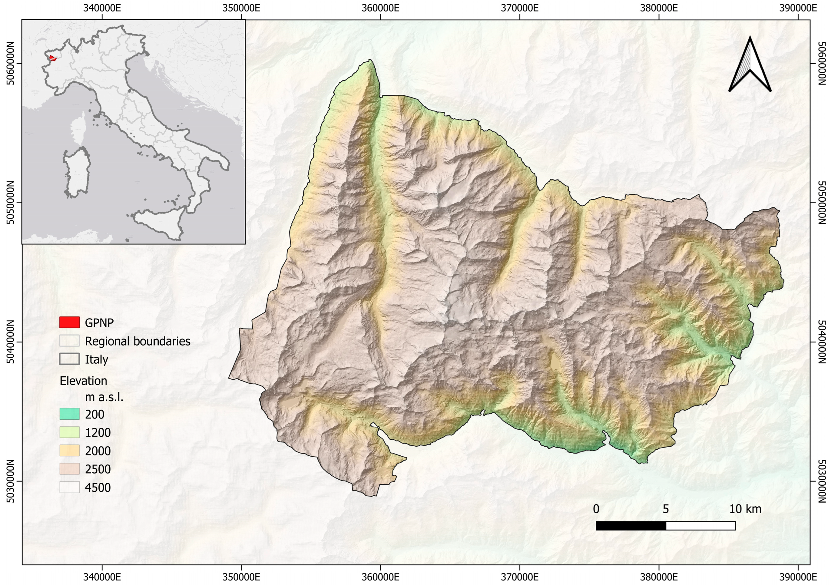
2.1. Study Area

The study area (Figure 1) is the Gran Paradiso National Park (GPNP), an alpine protected area that extends over 710 km2 in the North–West of the Italian Alps, between the regions of Piedmont and Aosta Valley, and presents a complex topography with numerous valleys and peaks up to over 4000 m a.s.l. The climate is alpine-continental type, with rigid winters and short summers and persisting snow above 2000 m a.s.l. from October/November until June. The GPNP is the first national park established in Italy, in 1922, in favor of the conservation of the ibex (Capra ibex). The Park Authority has been active in the area for 100 years, conducting numerous monitoring and research activities and collecting a huge amount of environmental data. The park territory has been influenced both in the past and in the present by human activities, which are concentrated in the valley floors in the winter and rise to high altitudes in the summer for tourists and pastoral activities [48].

2.2. Workflow

The geospatial dataset was built by collecting information layers from various sources, such as national and regional geoportals, regional environmental protection agencies (ARPA) websites, GPNP archives, and collaborative websites for sharing sports itineraries. Additional layers were obtained by using available orthoimages (Figure S1). All impacts were then normalized based on the relative intensity, where available, and weighted based on the temporal persistence of the impact itself. The cumulative impact map was then retrieved by summing all the impacts. The vulnerability map was estimated applying the LGRE methodology. Finally, the risk map was obtained by combining impact and vulnerability maps (Figure 2). More detailed information can be found in the following paragraphs.
All geodata were resampled on a 250 m × 250 m grid, spanning the whole GPNP area. Table 1 reports the dataset constructed and its time span covered.

2.2.1. Interviews and Questionnaires

In the period between August and September 2020, interviews were carried out with the managers of 11 mountain huts located in the GPNP. The aim of the interviews was on one hand to collect information on spatial distribution and relative intensity (such as number of tourists, number of kettles, or frequency of flights) of the impacts, and on the other, to investigate the managers’ perception of the impacts on the environment.
In addition, a questionnaire designed to collect information from tourists about their frequency of visiting and sports practice in the GPNP was compiled and distributed online. The questionnaire, distributed through a Google form, was freely filled out during the period between 1 August 2020 and 30 November 2020. A focus on the use of refuges and bivouacs and major trails and the conducted recreational activities was made. The questionnaire was promoted through the GPNP social media accounts (on Facebook and Instagram) and through a series of posters displayed in accommodation facilities (mountain huts, hotels, etc.) and other commercial activities in the area. A total of 314 questionnaires were filled out.

2.2.2. Worksites

The “Worksites” layer is considered useful to represent the impacts deriving from building interventions on the GPNP area [82]. The layer was obtained starting from the intervention authorization document provided by the GPNP, containing data relating to the works carried out in the last 40 years (1980–2020). A detailed analysis of each intervention was carried out resulting in a selection of the most significant interventions in terms of potential impacts on the landscape. The selection of interventions from the database was made arbitrarily, and minor interventions, e.g., gutter repair, were discarded, while new construction or other interventions with significant material movement and soil remodeling were retained. Those data containing geolocation information, also obtained with the help of input from shelter managers during the interviews, were included in a geospatial layer and considered in this study.

2.2.3. Derivations and Discharges

The point layer “Derivation and discharge” derives from the merge of different layers: (a) the shapefile provided by GPNP containing information on intake and discharge points on surface waters; (b) “Urban wastewater discharge”, “Discharge from the production site” and “Intake on surface water extracted” from the Water Resources Information System of the Piedmont Region (http://www.regione.piemonte.it/siriw/cartografia/mappa.do;jsessionid=71FF3621806243A7E72EB83D4BD22BC4.part212node12, accessed on 10 October 2020, accessed on 15 December 2019). The different point shapefiles were merged with no distinction since no information on the amount of intake or discharge was available.

2.2.4. Dams and Hydroelectric Power Plants

The dams were identified, at a detail scale up to 1:100, based on the photointerpretation of the most recent available orthophoto, acquired in 2012 and accessible through the Ministry of the Environment and the Protection of the Territory and the Sea—National Geoportal (http://wms.pcn.minambiente.it/ogc?map=/ms_ogc/WMS_v1.3/raster/ortofoto_colore_12.map&service=wms&request=getCapabilities&version=1.3.0, accessed on 10 October 2019).
The hydroelectric power plants layer was obtained from the geoportal of the Piedmont Region. Information on the hydroelectric power plants in the Piedmont area of the GPNP was supplemented with Lillaz hydroelectric power plant, located near the boundaries of the park in the Aosta Valley Region.

2.2.5. Imperviousness

The “Built-up” layer was derived from two datasets: the “Degree of Imperviousness”, distributed by the Land monitoring services of Copernicus (https://land.copernicus.eu/pan-european/high-resolution-layers/imperviousness/status-maps/imperviousness-density-2018, accessed on 29 November 2019), and the “building footprint” node of OpenStreetMap (OSM).
The “Degree of Imperviousness” is a thematic product that shows the sealing coverage in the range 0–100% for the period 2018, at a resolution of 10 m. This layer, created through the application of machine learning algorithms of the sealed soil directly from satellite images, resulted as inadequate in the case of sparse urban fabric; thus, this limit has been bridged by introducing the OpenStreetMap (OSM) layer with sparse buildings. This last layer is created not automatically, like the imperviousness layer, but through digitization by volunteer operators. The OSM layer, on the other hand, returns a polygon layer with the footprint of the building. Finally, the sealed ground was brought back to the grid at 250 × 250 m based on the percentage of sealed cells.

2.2.6. Road Network

The road network layer includes four types: local road, secondary extra-urban road, urban neighborhood street, and farm road [79]. The layer derives from the merge of the “Average Daily Traffic 2019” (ADT2019) from the regional geoportal of Piedmont (Geoportal Piedmont, https://www.geoportale.piemonte.it/geonetwork/srv/ita/catalog.search#/metadata/r_piemon:face619f-b974-4ed7-b0a1-ec6f42f9f0d9, accessed on 17 July 2020), and from the “road network” node acquired from OSM regarding the Aosta Valley side.
ADT2019 includes additional attributes of the linear component of the traffic graph, related to vehicular mobility (https://www.geoportale.piemonte.it/geonetwork/srv/ita/catalog.search#/metadata/r_piemon:face619f-b974-4ed7-b0a1-ec6f42f9f0d9, accessed on 25 July 2020). The average daily traffic value represents the number of vehicles that transit on the road element on average daily, in the reference year. It is distinguished by the type of vehicle, light or heavy, and expressed as number of vehicles per day. The “light” category includes all vehicles up to 3.5 t and 9 passengers, while the “heavy vehicles” category includes vehicles with a higher weight.
The most recent data available for the Aosta Valley were acquired from the Report on the State of the Environment (RSA) 2018–FLU_EM_001 (https://www.arpa.vda.it/en/relazione-stato-ambiente/archivio-rsa/xiii-relazione-sullo-stato-dell-ambiente-2018/1309-rsa-2018-flussi-di-materiali/rsa-2018-emissioni/3373-flussi-di-traffico-autoveicolare-fluem001, accessed on 23 August 2020), reporting on the motor vehicle traffic flows. The main routes of the regional road network are clustered into different categories characterized by different average daily traffic values for light and heavy vehicles. This information was merged and standardized in the final geodata reporting all the data into classes (Table 2).

2.2.7. Helicopter Flights

The starting information was contained in a shapefile owned by the park, of a punctual type, inherent to flights carried out in the period 2010–2019 by multiple actors.
Using the information “protocol number” and “route”, it was possible to define the routes followed by the individual flights. Each section was reconstructed, with the aid of a digital terrain model (DTM), calculating the path at minimum cost (slope and crossing on slope) in R environment [100], using the “leastcostpath” package [101], between the points of each section, arriving to obtain a reconstruction as realistic as possible of the route traveled by helicopters. Where the routes were not indicated, the single point was kept. We therefore arrived at two shapefiles, one of linear type, representing the routes flown over by helicopters, to which the information obtained from the interviews was added, and one of punctual type, relating to the data in which it was not possible to find information on the route traveled. Both files retain all original information, including the year when the flight occurred and overall days of flight.

2.2.8. Tourism and Sport Activities

The geospatial data related to tourism and sport activities have been obtained by combining information coming from different sources including data collected with the interviews of tourists and refuge managers. The following layers were produced:
  • Mountain huts and bivouacs: this layer contains the precise data of the location of mountain huts, bivouacs, hunting lodges, and park rangers’ lodges, digitized based on the orthophoto of 2012 with the help of various sources, such as the Gulliver site, OpenStreetMap, and the park website. The attributes considered concern name, type (mountain huts, bivouacs, hunting lodges, and park rangers’ lodges), municipality, region, and specific fields relating to the frequency of visits by tourists obtained with the data collected through the interviews. It reported the number of people who visit the refuge at least three times a year, more than once but less than three times a year, and never, derived from the tourist interviews. Moreover, the geodata reports the annual estimate of people who visit the refuge in summer and winter obtained through interviews with refuge managers.
  • Pathways: the geodata of the pathways were provided by the Park. To this were added the pathways that were absent in the first geodata of the data bank of the Aosta Valley path network, made public through a dedicated geo-navigator (https://catastosentieri.regione.vda.it, accessed on 28 August 2020), and from OSM. The information in the attribute table was subsequently standardized as much as possible. The attribute table is organized in a series of generic fields: id, num. section, name, municipality, length, min altitude, max altitude, the difference in height, section, average slope, typology, paving, gutters, edges, walls, state, signs, digressions, pastures, parks, classification, hunting roads, and royal mule tracks. In addition, two specific fields related to tourist attendance were available: a field already present in the geodata provided by the park and therefore only related to that part of the paths and a field containing the information derived from the questionnaire for tourists. They contain information only for the paths present in the initial geodata provided by the park, on which the questionnaire was built.
  • Sport activities: the information relating to sports was taken from the Gulliver website (https://www.gulliver.it, accessed on 12 December 2020), an outdoor community where users share information on itineraries where they can practice different types of sports. On this platform it is possible to set geographic filters by sporting activity. Each itinerary in Gulliver’s database was then digitized, where the description was clear enough to allow a correct location or the track was downloaded, when available, resulting in the following geodata: climbing, bouldering, equipped cragging, trekking (i.e., pathways), mountain biking, canyoning (summer sports), alpine/steep skiing, snowshoeing, icefalls climbing (winter sports). The shapefile relating to the skiing facilities was provided by the park, and no changes have been made.

2.2.9. Overgrazing

The “Overgrazing” geodata was produced starting from the Excel database provided by park with the information about the area covered by pastures between 2000 and 2018. Databases for every year were merged and a unique identifier was created for each pasture, combining the id and “year”. Subsequently, the records without references to the grid cells were deleted in case of incomplete or absent geographical indications or were completed with reference cells in case of sufficient information was provided. The final database was processed in R to report each pasture data within the selected grid cell to obtain a shapefile for each individual pasture, subsequently merged into a single geodata in which the pastures are layered. Through geoprocessing, the total area of each pasture was then calculated. Grazing activity, if well managed, does not in itself constitute an impact but, on the contrary, is desirable for the maintenance of biodiversity. On the other hand, if it is poorly managed it constitutes a negative impact. For this reason, it is useful to weight the impact of pastures where overgrazing has occurred and exclude all other grazing activities. No applicable methods have emerged from the scientific literature to estimate the grazing capacity of the pastures on a large scale, so we made use of the gray literature and of the regulations deriving from local management policies, such as the Rural Development Plans of Piedmont and the Aosta Valley. Overgrazing events were identified as those above the threshold of 0.5 livestock units per hectare per year (LU/ha/year) indicated for alpine pasture zoning for the Aosta Valley side and 0.6 for the Piedmont side.

2.2.10. Forest Cuts

Through the interviews, it was not possible to obtain any data relating to forest cuts because this information does not concern mountain hut managers. The only data available are in the intervention authorization file of the park, from which it is possible to filter, among all the intervention types, e.g., fencing or building repair, the forest cuts, for a total of 44 forest cutting operations. The permission database was deemed valid because illegal cutting is implausible given the surveillance by the park authority. However, only 6 interventions report sufficient information for correct geo-localization. In the other cases, due to the partial description of the place of intervention, it was not possible to digitize this data. Given the partiality of the information relating to the “Forest cuts” geodata, it was decided to completely exclude this pressure factor from the analysis.

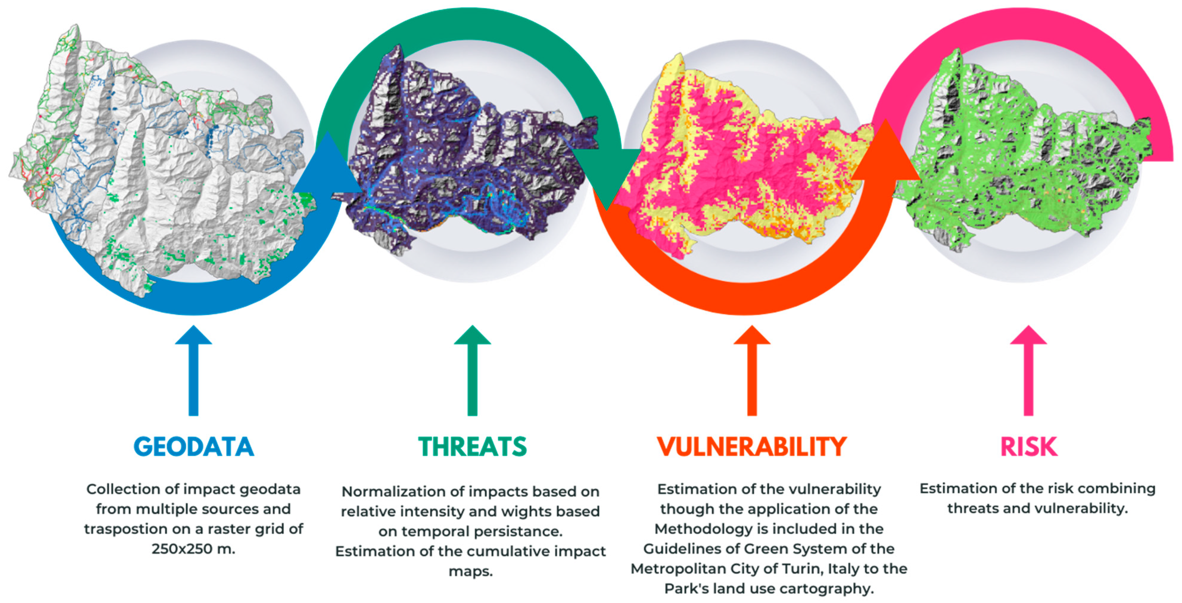
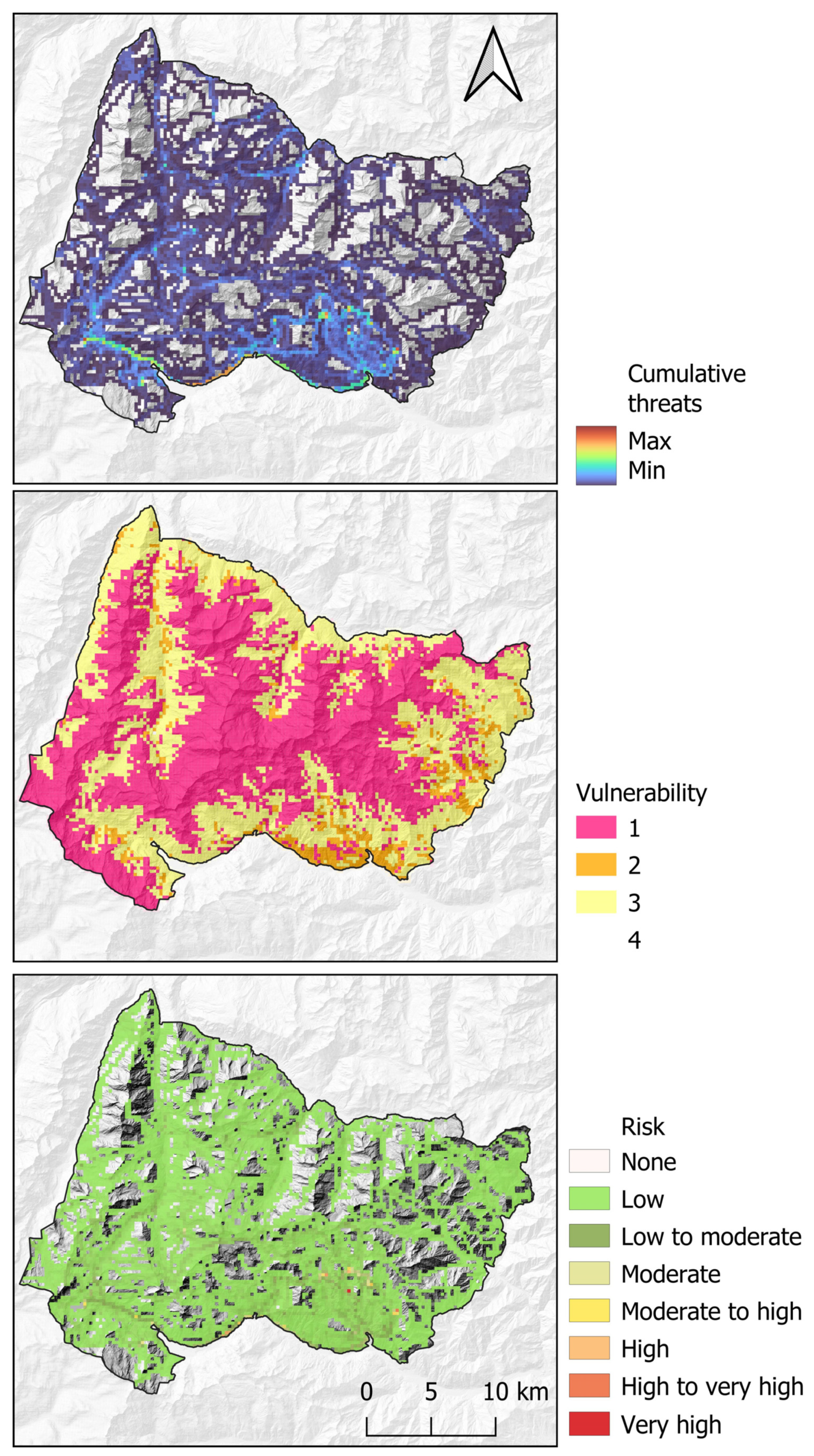
2.3. Estimate of the Threats Value

2.3.1. Normalization and Weighting of Threats Intensity

All the quantitative data related to specific threats have been normalized by considering the ratio of each threat intensity with respect to its maximum value. This procedure resulted in a standardized scale of 0–1. If no quantitative information is available, the value assigned is 1 to consider the presence of the specific threat and 0 in the case of absence (Table 3).
In the literature, no impact values were found to express quantitatively the different sources of pressure. In similar studies, the analysis of pressures was carried out by using weights of individual impacts inferred through expert evaluation. In this study, the assignment of a weight value for each impact was based on the temporal frequency of the impact itself: constant impacts over time have a value of 1, e.g., dams and hydroelectric plants, while 0 is considered for impacts that do not persist at all, e.g., winter bivouacs. Intermediate values represent intermediate persistence times considered over the day and/or year by type (Table 4). For example, worksites have a limited duration in the annual time but high daily in the time of occurrence, and thus 0.8 was assigned. In contrast, bouldering is an activity that lasts a few hours during the day and presumably does not occur every day, so it was assigned the value 0.2.

2.3.2. Cumulative Analysis of Threats

The cumulative analysis was performed summing all the impacts that persist for each cell of the analyzed area (on a 250 m × 250 m grid).

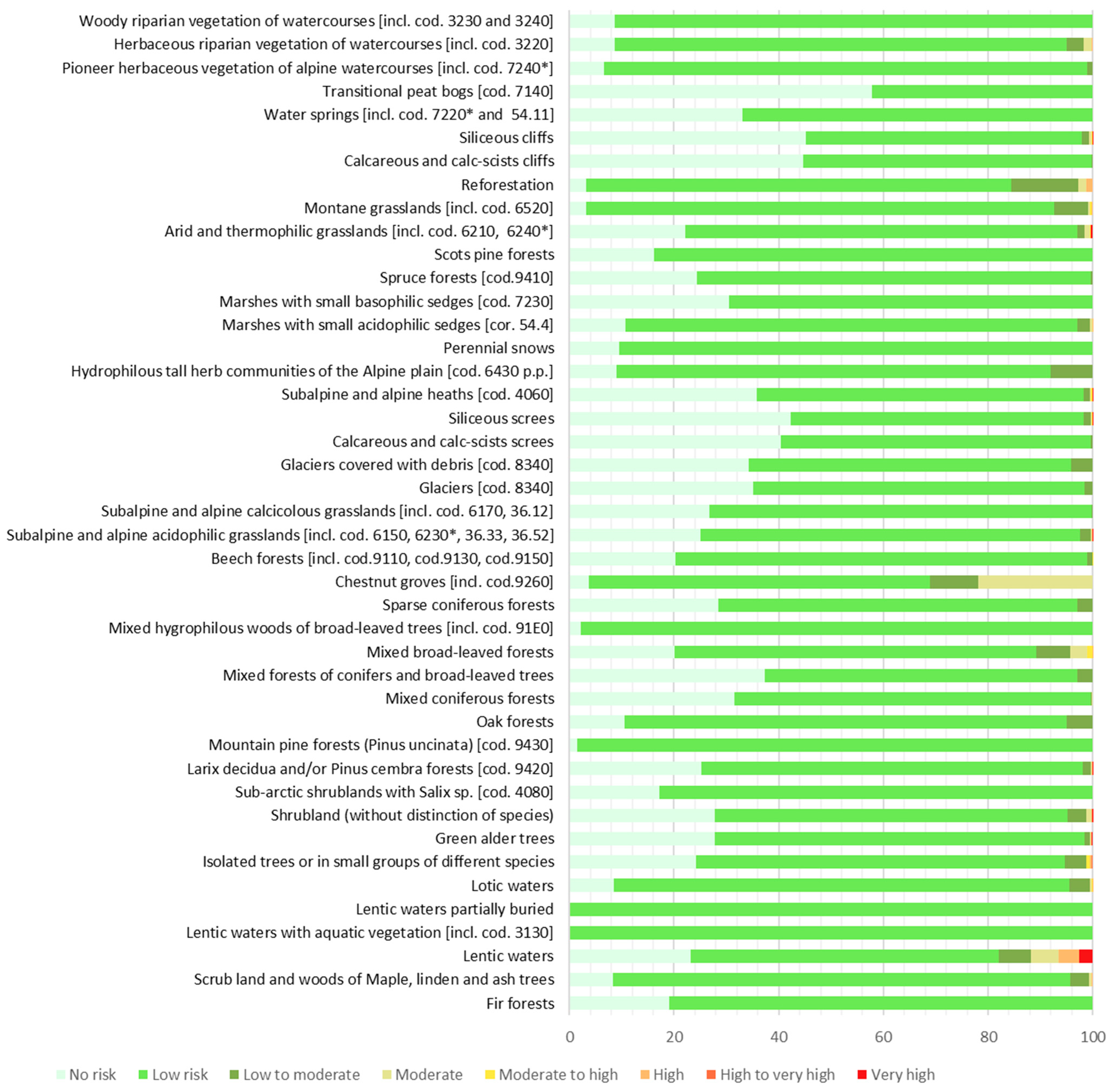
2.4. Vulnerability and Risk Assessment

The vulnerability is inferred using the ecological-environmental assessment values of the fragility parameter assigned to the legend classes of the Land Cover Piemonte (LCP) 2010 cartography, translating them into the land-use cartography of the park (see Table S1). The approach adopted for the level of fragility assignation is based on expert evaluation as reported by the Ecological Network methodology developed by the Metropolitan City of Turin and ENEA [102]. The levels of fragility, defined as the inverse of resilience, were assigned through expert knowledge considering the following criteria:
  • Level 1: land-use classes characterizing both natural environments with very low resilience and semi-natural environments with significant anthropic determinism that are easily impacted (e.g., rocky areas, artificial water basins, areas with sparse vegetation).
  • Level 2: natural and semi-natural land-use classes which can be considered poorly resilient with respect to the pressures deriving from anthropic disturbance (e.g., areas with shrub vegetation in natural evolution, pastures).
  • Level 3: natural land-use classes with good resilience (e.g., climatic tree formations).
  • Level 4: all the land-use classes with total anthropogenic determinism (e.g., most of the crops and the types of artificial land use).
The 4 levels of fragility were converted on a scale from 0, for artificial and agricultural areas, to a maximum of 1, for highly vulnerable land-use types.
To associate the classification of the GPNP cartography with the Piedmont Land Cover classification (LCP) [103], and, thus, to translate the fragility values associated with the latter, we proceeded by comparing the correspondence between the two cartographies in a GIS environment. Both the land-use layers were made at an analysis scale of 1:10,000, and, in some cases, up to 1:2000 as regards the park map. The park map was created through an analysis of the vegetation starting from aerial photogrammetric surveys (years 2005–2012), identifying the different polygons and attributing them to the different subgroups (and in some cases to more detailed classifications) with the help of the geological map and the forest typology map; the direct knowledge of the vegetation of the territory, organized in the databases of the park’s botanical service, is also of great importance for the attribution. LCP, released in 2010, derives from the harmonization and integration of data present in archives and maps already existing in the Piedmont Region, following specific analyses and processing in the final data feed. The scales of analysis and the reference years of the source data are superimposable; therefore, it is possible to make a comparison, albeit indicative, between the two maps. For each type of land cover in the park cartography, the correspondence with the land cover surfaces of LCP, found through a spatial analysis, is shown in the Supplementary Materials. For example, the cartography class of the “Fir trees” park overlaps by 90% with the LCP class “3121-Fir trees”, which is associated with a fragility value of 3, by 8% with the LCP class “3124-Woods of larch and/or stone pine”, with a fragility value of 3, and by 2% to the class “2310-Stable meadows and pastures”, with a fragility value of 2.
Finally, by combining the impact map with the vulnerability, it is possible to obtain the risk map by using the following equation:
Risk = Vulnerability × Threat
The conservation value was not considered in the Equation (1) because, since this is an area protected both on a national and European level (Special Protection Area), the conservation value is to be assumed maximum in any case.

3. Results

Figure 3 shows the results of the methodologies applied to assess, respectively, the cumulative impacts (top), vulnerability (middle), and risk (bottom) on the GPNP area.
High values indicate areas where multiple pressure factors overlap. The threat values range from 0 to 8.6. The vulnerability values range from 0 to 4. The risk values obtained were divided into the following risk classes: 0 = no risk; 0–1.5 = low risk; 1.5–3 = low to moderate risk; 3–4.5 = moderate risk; 4.5–6 = moderate to high risk; 6–7.5 = high risk; 7.5–8 = high to very-high risk; >8 = very-high risk. The risk map obtained shows that most of the park’s territory (63%) falls into areas with low risk, followed by areas with no risk (35% of the territory), i.e., with no anthropogenic activity insisting on those areas. These two classes together cover about the 98% of the park. The remaining 2% is distributed among the other classes (Table 5).
Overall, most of the habitat surfaces are, as a result, affected by the low-risk or no-risk classes (Figure 4). However, no habitat typology is completely unaffected by threats. On the other hand, “Lentic waters with aquatic vegetation [incl. cod. 3130]” and “Lentic waters partially buried” fall entirely in the low-risk class. Additionally, the habitats “Mountain pine forests (Pinus uncinata) [cod. 9430]” and “Mixed hygrophilous woods of broad-leaved trees [incl. cod. 91E0]” are almost entirely in the low-risk class, with respectively only 1 and 2% in the no-risk class. Following this, we found “Montane grasslands [incl. cod. 6520]” and “Chestnut groves [incl. cod.9260]”, “Marshes with small acidophilic sedges [cor. 54.4]”, “Pioneer herbaceous vegetation of alpine watercourses [incl. cod. 7240*]”, “Herbaceous riparian vegetation of watercourses [incl. cod. 3220]”, and “Woody riparian vegetation of watercourses [incl. cod. 3230 and 3240]” with less than 10% at no risk. The only vegetation type that falls more than half in the no-risk class is the “Transitional peat bogs [cod. 7140]” with 58%, followed by the “Calcareous and calc-scists cliffs” and the “Siliceous cliffs”, both with 45%, and the screes, “Siliceous screes” and “Calcareous and calc-scists screes”, with, respectively, 42 and 40%. The other vegetation types are included for a range between 10 and 40% in this class. The low-risk class is the most represented; in fact, most of the surfaces fall into this category. The other risk classes affect smaller portions of the park’s territory.
The low to moderate class affects the 13% of the “Reforestation” areas, and the 9% of “Chestnut groves [incl. cod.9260]”, followed by the 8% of “Hydrophilous tall herb communities of the Alpine plain [cod. 6430 p.p.]”, the 7% of “Montane grasslands [incl. cod. 6520]”, and under 6% to 0% of the other vegetation types. The 22% of “Chestnut groves [incl. cod.9260]” falls in the moderate risk class. The moderate-to-high-risk class is almost empty, affecting 2 to 0% of the different land cover types, as well as the high-, the high-to-very-high and very-high classes. The “Lentic waters” are the land cover type most affected by risks, with 3% in the very-high risk, 4% in high risk, 5% in moderate risk, 6% in low to moderate risk, and the rest in low- or no-risk classes. This is due to the presence of the dams and hydroelectric plants that require this land cover type.

4. Discussion

Through a preliminary analysis, the park’s managers have identified the stressors that insist on the study area: helicopter flights, worksites, forest cuts, grazing and other agro-pastoral activities, tourist impact (tourism entities and sports activities on trails and shelters), road traffic, stream uptake and derivation, dams and hydroelectric plants, and urban fabric and infrastructure.
The information available regarding the location and intensity of the threats identified was collected and digitized from various sources, including through the conduct of interviews, and stored in a geodatabase.
At this stage, the pressure “Forest cuts” were excluded from the analysis due to the lack of data. Pressures were normalized in a range between 0 and 1 based on their intensity and weighted based on the temporal frequency of the impact itself. Starting from the park’s land-use/land-cover cartography, a vulnerability map was then extracted, expressed in a range between 0 (no vulnerability) and 1 (maximum vulnerability) using the methodology proposed by ENEA and the CMTo for the Green Guidelines.
Finally, by combining the pressure maps and the vulnerability map, the risk map was calculated on a grid of the park of 250 × 250 m. The risk map, therefore, represents the additive sum of the values of the multiple pressures, normalized and weighted, which reside in each cell, multiplied by the vulnerability value of the corresponding habitat types.
The values of the risk map have been divided into eight risk level classes. The classes represent the spatial concentration of pressure factors as a general disturbance on habitat and animal species and are therefore indicative of areas in which disturbance types present in the park territory are co-present.
Overall, the analysis highlights good management of the activities in the park, evidenced by the absence of environmental emergencies in terms of habitats subjected to high pressures, as also found by other studies [40].
The activities that determine anthropic frequentation are spread throughout the territory, and there are few areas completely free of pressure factors. Nevertheless, there are no habitats characterized by a significant percentage extension in high-risk areas. The type with a non-negligible percentage in areas with a moderate to high risk level is the “Lentic waters” class, which, however, includes both natural and artificial water basins, created by the presence of dams, while the other classes present negligible levels of risk.
Finally, it should be noted that some natural environmental typologies fall 100% in areas with a different level of risk; however, the risk is not zero, e.g., the “Lentic waters with aquatic vegetation [incl. cod. 3130]” and the “Lentic waters partially buried”. Additionally, for the most falling in some risk class there are the “Mountain pine forests (Pinus uncinata) [cod. 9430]”, the “Mixed hygrophilous woods of broad-leaved trees [incl. cod. 91E0]”, the “Montane grasslands [incl. cod. 6520]”, “Chestnut groves [incl. cod.9260]”, “Marshes with small acidophilic sedges [cor. 54.4]”, “Pioneer herbaceous vegetation of alpine watercourses [incl. cod. 7240*]”, “Herbaceous riparian vegetation of watercourses [incl. cod. 3220]”, and “Woody riparian vegetation of watercourses [incl. cod. 3230 and 3240]”.
The methodological approach used has already found many applications in natural areas, especially in marine and coastal areas; however, there are no guidelines for the construction of the pressure factor dataset or the related threat estimate. This method is therefore still under development and demonstrates the need to deepen the study of decision support tools and specific methodologies to support planning in parks and nature reserves and is crucial for effective protected area management [104].
The impact geodatabase was constructed with data from multiple sources, with different temporal coverage, collected and harmonized. Some represent a snapshot of a specific moment in which the data was acquired while others span 20 years (from 2000 to 2020). However, the heterogeneity of the data used does not represent a limit for the analysis thanks to the normalization and harmonization in the grid at 250 × 250 m. On the contrary, gaps in the stressor geodatabase are a common problem affecting cumulative impact analysis both on large [105] and fine scales [15]. In this study, for example, forest cuts or, in general, areas where it was not possible to geolocate impacts, made the starting database non-exhaustive. Thus, although an operational tool for park managers would require further studies, the present work represents a useful preliminary analysis aiming to highlight gaps in both available data and methodological approach.
This study represents a first attempt to map the risks occurring in the park territory for habitat and species. Overall, a cumulative impact analysis can provide valuable insights into the potential effects of multiple stressors on ecosystems. However, it is important to recognize the limitations of this approach and to use caution when interpreting the results of the analysis. One of the key limitations of a cumulative impact analysis is that the interactions between different stressors are often non-additive. This means that the combined effect of two or more stressors is not simply the sum of their individual effects. Instead, the interaction between the stressors may result in a synergistic effect that is greater than the sum of their individual effects. Alternatively, the interaction may result in an antagonistic effect that is less than the sum of their individual effects [15]. Another limitation of a cumulative impact analysis is that the response of vegetation communities to stressors is often non-linear. This means that the magnitude of the stressor and the response of the ecosystem is not necessarily linear. Instead, the response of the ecosystem may be exponential, logarithmic, or exhibit other complex patterns. These non-linear responses can make it difficult to predict the effects of stressors on habitats [15,106]. In a future deeper analysis, these shortcomings should be considered to obtain a more realistic risk map.
In the same way, the vulnerability weights associated with each stressor/habitat combination should be considered in a future improvement of the present study, in which they were assumed to be all equal. These weights are used to reflect the relative vulnerability of different habitats to different threats. However, there is limited knowledge on specific interactions between most stressor/habitat combinations [106], so this point is still tough. Another key challenge is in determining the threshold at which the functionality of an ecosystem is compromised. This threshold will vary depending on the specific ecosystem being studied and the stressors that are impacting it. However, determining this threshold can be challenging, particularly when there is limited information available on the long-term effects of multiple stressors on ecosystems [15].
Finally, one of the significant limitations of a cumulative impact analysis is the challenge of validating the predictions made by the analysis. This is particularly challenging when the analysis is based on complex models that incorporate multiple stressors and non-linear responses. Ground truth data require long-term monitoring of ecosystems to assess the accuracy of the predictions made by the analysis. However, such monitoring can be expensive and time-consuming, making it challenging to validate the results of a cumulative impact analysis [16].

5. Conclusions

The present study, based on a cumulative multi-pressure assessment model generated by anthropogenic attendance, is proposed as a support methodology for decision-makers and planners in the analysis of the current areas at risk of deterioration and can be used to identify management priorities in the study area.
To adapt this method to other study areas, the pressure considered should be selected specifically based on an in-depth knowledge of the territory and of the threats present as well as the availability of the data. However, the weights for threats and vulnerability could be quantified based on an expert evaluation or on the basis of studies conducted on the relationship between specific threat/habitat combinations.
A possible future development of this study is the comparison with the map of impacts and risks obtained with the map of land cover changes that have occurred to highlight any correlations and, subsequently, use the data obtained to refine the vulnerability weights for each stressor/habitat combination, which is also useful for modeling future land cover and habitat change scenarios using software such as InVEST (Integrated Valuation of Ecosystem Services and Tradeoffs) [107] and integrating climate change models not captured by this study. Furthermore, it would be desirable to enrich the datasets of the pressure factors used with threats for which no data were found in this study, such as forest cuts and the distribution of invasive alien plant species.
Finally, spatial threat propagation models based on pressure-factor-specific simulations could be included to refine the model, which was assumed to be linear in this study.
In summary, despite the above uncertainties, this study, the results of which confirm the effectiveness of the park’s protection policies, is significant for assessing the ecological risk present in the GPNP based on the cumulative pressure analysis method and can provide valid support for territorial protection and management.

Supplementary Materials

The following supporting information can be downloaded at: https://www.mdpi.com/article/10.3390/land12061124/s1, Table S1: Transcoding between the legend of the park cartography and the legend of Land Cover Piemonte 2010. Figure S1: Impacts of geodata mapped in this study.

Author Contributions

Conceptualization, C.R.; methodology, C.R.; formal analysis, C.R.; investigation, C.R.; data curation, C.R.; writing—original draft preparation, C.R., M.A., M.R.M. and C.S.; writing—review and editing, C.R., M.A., M.R.M. and C.S.; visualization, C.R.; supervision, M.A., M.R.M. and C.S. All authors have read and agreed to the published version of the manuscript.

Funding

This research received no external funding.

Institutional Review Board Statement

Not applicable.

Informed Consent Statement

Not applicable.

Acknowledgments

The main thanks go to the park staff, Ramona Viterbi and Andrea Mainetti, and to the Gran Paradiso National Park Management, which provided the data and insights into the methodology and threats that persist in the Park’s territory. We would also like to thank Simone Ravetto Enri for the valuable suggestions on overgrazing detection.

Conflicts of Interest

The authors declare no conflict of interest.

References

  1. Slaymaker, O.; Embleton-Hamann, C. Advances in Global Mountain Geomorphology. Geomorphology 2018, 308, 230–264. [Google Scholar] [CrossRef]
  2. Butler, D.R.; Malanson, G.P.; Resler, L.M.; Walsh, S.J.; Wilkerson, F.D.; Schmid, G.L.; Sawyer, C.F. Chapter 4 Geomorphic Patterns and Processes at Alpine Treeline. Dev. Earth Surf. Process. 2009, 12, 63–84. [Google Scholar] [CrossRef]
  3. Opedal, Ø.H.; Armbruster, W.S.; Graae, B.J. Linking Small-Scale Topography with Microclimate, Plant Species Diversity and Intra-Specific Trait Variation in an Alpine Landscape. Plant. Ecol. Divers. 2015, 8, 305–315. [Google Scholar] [CrossRef] [Green Version]
  4. Fedele, F.G. Toward a Human Ecology of Mountains. Curr. Anthr. 1984, 25, 688–691. [Google Scholar] [CrossRef]
  5. Gambari, F.M.; Ferrero, L.; Padovan, S. (Eds.) Pionieri Delle Alpi: Il Pieno Neolitico tra le Alpi Occidentali; Soprintendenza Archeologia del Piemonte: Turin, Italy, 2016. [Google Scholar]
  6. Volume XVI 1992—Il Popolamento Delle Alpi Occidentali—Museo Civico Di Scienze Naturali Di Bergamo. Available online: https://www.museoscienzebergamo.it/senza-categoria/volume-xvi-1992-il-popolamento-delle-alpi-occidentali/ (accessed on 21 July 2022).
  7. Dirnböck, T.; Dullinger, S.; Grabherr, G. A Regional Impact Assessment of Climate and Land-Use Change on Alpine Vegetation. J. Biogeogr. 2003, 30, 401–417. [Google Scholar] [CrossRef]
  8. Carcaillet, C.; Brun, J.-J. Changes in Landscape Structure in the Northwestern Alps over the Last 7000 Years: Lessons from Soil Charcoal. J. Veg. Sci. 2000, 11, 705–714. [Google Scholar] [CrossRef]
  9. Grime, J.P. Vegetation Classification by Reference to Strategies. Nature 1974, 250, 26–31. [Google Scholar] [CrossRef]
  10. Zhang, J.T.; Xu, B.; Li, M. Vegetation Patterns and Species Diversity Along Elevational and Disturbance Gradients in the Baihua Mountain Reserve, Beijing, China. Mt. Res. Dev. 2013, 33, 170–178. [Google Scholar] [CrossRef]
  11. Niu, L.; Cheng, Z. Impact of Tourism Disturbance on Forest Vegetation in Wutai Mountain, China. Environ. Monit. Assess. 2019, 191, 1–11. [Google Scholar] [CrossRef]
  12. Journal, A.I.; Klug, B.; Scharfetter-Lehrl, G.; Scharfetter, E. Effects of Trampling on Vegetation above the Timberline in the Eastern Alps, Austria. Arctic Antarct. Alp. Res. 2018, 34, 377–388. [Google Scholar] [CrossRef]
  13. Rusch, G.M.; Pausas, J.G.; Lepš, J. Plant Functional Types in Relation to Disturbance and Land Use: Introduction. J. Veg. Sci. 2003, 14, 307–310. [Google Scholar] [CrossRef]
  14. Piragnolo, M.; Pirotti, F.; Guarnieri, A.; Vettore, A.; Salogni, G. Geo-Spatial Support for Assessment of Anthropic Impact on Biodiversity. ISPRS Int. J. Geoinf. 2014, 3, 599–618. [Google Scholar] [CrossRef] [Green Version]
  15. Ban, N.C.; Alidina, H.M.; Ardron, J.A. Cumulative Impact Mapping: Advances, Relevance and Limitations to Marine Management and Conservation, Using Canada’s Pacific Waters as a Case Study. Mar. Policy 2010, 34, 876–886. [Google Scholar] [CrossRef]
  16. Clark, D.; Goodwin, E.; Sinner, J.; Ellis, J.; Singh, G. Validation and Limitations of a Cumulative Impact Model for an Estuary. Ocean. Coast. Manag. 2016, 120, 88–98. [Google Scholar] [CrossRef]
  17. Caniani, D.; Labella, A.; Lioi, D.S.; Mancini, I.M.; Masi, S. Habitat Ecological Integrity and Environmental Impact Assessment of Anthropic Activities: A GIS-Based Fuzzy Logic Model for Sites of High Biodiversity Conservation Interest. Ecol. Indic. 2016, 67, 238–249. [Google Scholar] [CrossRef]
  18. Harik, G.; Alameddine, I.; Maroun, R.; Rachid, G.; Bruschi, D.; Astiaso Garcia, D.; El-Fadel, M. Implications of Adopting a Biodiversity-Based Vulnerability Index versus a Shoreline Environmental Sensitivity Index on Management and Policy Planning along Coastal Areas. J. Environ. Manag. 2017, 187, 187–200. [Google Scholar] [CrossRef]
  19. Halpern, B.S.; Walbridge, S.; Selkoe, K.A.; Kappel, C.V.; Micheli, F.; D’agrosa, C.; Bruno, J.F.; Casey, K.S.; Ebert, C.; Fox, H.E.; et al. A Global Map of Human Impact on Marine Ecosystems. Science 2008, 319, 948–952. [Google Scholar] [CrossRef] [Green Version]
  20. Stelzenmüller, V.; Coll, M.; Mazaris, A.D.; Giakoumi, S.; Katsanevakis, S.; Portman, M.E.; Degen, R.; Mackelworth, P.; Gimpel, A.; Albano, P.G.; et al. A Risk-Based Approach to Cumulative Effect Assessments for Marine Management. Sci. Total Environ. 2018, 612, 1132–1140. [Google Scholar] [CrossRef]
  21. Brignon, J.M.; Lejart, M.; Nexer, M.; Michel, S.; Quentric, A.; Thiebaud, L. A Risk-Based Method to Prioritize Cumulative Impacts Assessment on Marine Biodiversity and Research Policy for Offshore Wind Farms in France. Environ. Sci. Policy 2022, 128, 264–276. [Google Scholar] [CrossRef]
  22. Stockbridge, J.; Jones, A.R.; Gillanders, B.M. A Meta-Analysis of Multiple Stressors on Seagrasses in the Context of Marine Spatial Cumulative Impacts Assessment. Sci. Rep. 2020, 10, 11934. [Google Scholar] [CrossRef]
  23. Murphy, G.E.P.; Kelly, N.E.; Lotze, H.K.; Wong, M.C. Incorporating Anthropogenic Thresholds to Improve Understanding of Cumulative Effects on Seagrass Beds. Facets 2022, 7, 966–987. [Google Scholar] [CrossRef]
  24. Boyd, P.W.; Hutchins, D.A. Understanding the Responses of Ocean Biota to a Complex Matrix of Cumulative Anthropogenic Change. Mar. Ecol. Prog. Ser. 2012, 470, 125–135. [Google Scholar] [CrossRef] [Green Version]
  25. Korpinen, S.; Andersen, J.H. A Global Review of Cumulative Pressure and Impact Assessments in Marine Environments. Front. Mar. Sci. 2016, 3, 153. [Google Scholar] [CrossRef] [Green Version]
  26. Stelzenmüller, V.; Coll, M.; Cormier, R.; Mazaris, A.D.; Pascual, M.; Loiseau, C.; Claudet, J.; Katsanevakis, S.; Gissi, E.; Evagelopoulos, A.; et al. Operationalizing Risk-Based Cumulative Effect Assessments in the Marine Environment. Sci. Total Environ. 2020, 724, 138118. [Google Scholar] [CrossRef] [PubMed]
  27. Halpern, B.S.; Frazier, M.; Potapenko, J.; Casey, K.S.; Koenig, K.; Longo, C.; Lowndes, J.S.; Rockwood, R.C.; Selig, E.R.; Selkoe, K.A.; et al. Spatial and Temporal Changes in Cumulative Human Impacts on the World’s Ocean. Nat. Commun. 2015, 6, 7615. [Google Scholar] [CrossRef] [PubMed] [Green Version]
  28. Stock, A.; Micheli, F. Effects of Model Assumptions and Data Quality on Spatial Cumulative Human Impact Assessments. Glob. Ecol. Biogeogr. 2016, 25, 1321–1332. [Google Scholar] [CrossRef]
  29. Trew, B.T.; Grantham, H.S.; Barrientos, C.; Collins, T.; Doherty, P.D.; Formia, A.; Godley, B.J.; Maxwell, S.M.; Parnell, R.J.; Pikesley, S.K.; et al. Using Cumulative Impact Mapping to Prioritize Marine Conservation Efforts in Equatorial Guinea. Front. Mar. Sci. 2019, 6, 717. [Google Scholar] [CrossRef]
  30. Wyatt, K.H.; Griffin, R.; Guerry, A.D.; Ruckelshaus, M.; Fogarty, M.; Arkema, K.K. Habitat Risk Assessment for Regional Ocean Planning in the U.S. Northeast and Mid-Atlantic. PLoS ONE 2017, 12, e0188776. [Google Scholar] [CrossRef]
  31. Arkema, K.K.; Verutes, G.; Bernhardt, J.R.; Clarke, C.; Rosado, S.; Canto, M.; Wood, S.A.; Ruckelshaus, M.; Rosenthal, A.; McField, M.; et al. Assessing Habitat Risk from Human Activities to Inform Coastal and Marine Spatial Planning: A Demonstration in Belize. Environ. Res. Lett. 2014, 9, 114016. [Google Scholar] [CrossRef] [Green Version]
  32. Fierro, P.; Valdovinos, C.; Arismendi, I.; Díaz, G.; Ruiz De Gamboa, M.; Arriagada, L. Assessment of Anthropogenic Threats to Chilean Mediterranean Freshwater Ecosystems: Literature Review and Expert Opinions. Environ. Impact Assess. Rev. 2019, 77, 114–121. [Google Scholar] [CrossRef]
  33. Macdiarmid, A.; Mckenzie, A.; Sturman, J.; Beaumont, J.; Mikaloff-Fletcher, S.; Dunne, J. Assessment of Anthropogenic Threats to New Zealand Marine Habitats New Zealand Aquatic Environment and Biodiversity Report No. 93 2012; Ministry of Agriculture and Forestry: Wellington, New Zealand, 2012. Available online: http://www.maf.govt.nz/news-resources/publications.aspx (accessed on 22 May 2023).
  34. Depellegrin, D.; Menegon, S.; Gusatu, L.; Roy, S.; Misiunė, I. Assessing Marine Ecosystem Services Richness and Exposure to Anthropogenic Threats in Small Sea Areas: A Case Study for the Lithuanian Sea Space. Ecol. Indic. 2020, 108, 105730. [Google Scholar] [CrossRef]
  35. Sajjad, M.; Li, Y.; Tang, Z.; Cao, L.; Liu, X. Assessing Hazard Vulnerability, Habitat Conservation, and Restoration for the Enhancement of Mainland China’s Coastal Resilience. Earths Future 2018, 6, 326–338. [Google Scholar] [CrossRef] [Green Version]
  36. Halpern, B.S.; Kappel, C.V.; Selkoe, K.A.; Micheli, F.; Ebert, C.M.; Kontgis, C.; Crain, C.M.; Martone, R.G.; Shearer, C.; Teck, S.J. Mapping Cumulative Human Impacts to California Current Marine Ecosystems. Conserv. Lett. 2009, 2, 138–148. [Google Scholar] [CrossRef]
  37. Seitz, N.E.; Westbrook, C.J.; Noble, B.F. Bringing Science into River Systems Cumulative Effects Assessment Practice. Environ. Impact Assess. Rev. 2011, 31, 172–179. [Google Scholar] [CrossRef]
  38. Halpern, B.S.; Selkoe, K.A.; Micheli, F.; Kappel, C.V. Evaluating and Ranking the Vulnerability of Global Marine Ecosystems to Anthropogenic Threats. Conserv. Biol. 2007, 21, 1301–1315. [Google Scholar] [CrossRef] [PubMed]
  39. Gao, Y.; Li, R.; Gao, H.; Hou, C.; Jin, S.; Ye, J.; Na, G. Spatial Distribution of Cumulative Impact on Terrestrial Ecosystem of the Fildes Peninsula, Antarctica. J. Environ. Manage 2021, 279, 111735. [Google Scholar] [CrossRef]
  40. Egarter Vigl, L.; Marsoner, T.; Schirpke, U.; Tscholl, S.; Candiago, S.; Depellegrin, D. A Multi-Pressure Analysis of Ecosystem Services for Conservation Planning in the Alps. Ecosyst. Serv. 2021, 47, 101230. [Google Scholar] [CrossRef]
  41. O’Bryan, C.J.; Allan, J.R.; Holden, M.; Sanderson, C.; Venter, O.; Di Marco, M.; McDonald-Madden, E.; Watson, J.E.M. Intense Human Pressure Is Widespread across Terrestrial Vertebrate Ranges. Glob. Ecol. Conserv. 2020, 21, e00882. [Google Scholar] [CrossRef]
  42. Gong, M.; Fan, Z.; Zhang, X.; Liu, G.; Wen, W.; Zhang, L. Measuring the Effectiveness of Protected Area Management by Comparing Habitat Utilization and Threat Dynamics. Biol. Conserv. 2017, 210, 253–260. [Google Scholar] [CrossRef]
  43. Sobhani, P.; Esmaeilzadeh, H.; Barghjelveh, S.; Sadeghi, S.M.M.; Marcu, M.V. Habitat Integrity in Protected Areas Threatened by Lulc Changes and Fragmentation: A Case Study in Tehran Province, Iran. Land 2022, 11, 6. [Google Scholar] [CrossRef]
  44. Adem Esmail, B.; Geneletti, D. Multi-Criteria Decision Analysis for Nature Conservation: A Review of 20 Years of Applications. Methods Ecol. Evol. 2018, 9, 42–53. [Google Scholar] [CrossRef] [Green Version]
  45. Vaissi, S.; Sharifi, M. Integrating Multi-Criteria Decision Analysis with a GIS-Based Siting Procedure to Select a Protected Area for the Kaiser’s Mountain Newt, Neurergus Kaiseri (Caudata: Salamandridae). Glob. Ecol. Conserv. 2019, 20, e00738. [Google Scholar] [CrossRef]
  46. Cegan, J.C.; Filion, A.M.; Keisler, J.M.; Linkov, I. Trends and Applications of Multi-Criteria Decision Analysis in Environmental Sciences: Literature Review. Environ. Syst. Decis. 2017, 37, 123–133. [Google Scholar] [CrossRef]
  47. Alberico, S.; Grasso, S.; Vayr, P.; Minciardi, M.R.; Rossi, G.; Ciadamidaro, S.; Quaglio, G. Linee Guida per Il Sistema Del Verde; Provincia di Torino: Torino, Italy; Available online: http://www.cittametropolitana.torino.it/cms/territorio-urbanistica/sistema-verde/sistema-verde (accessed on 22 May 2023).
  48. Siniscalco, C. Impact of Tourism on Flora, and Vegetation in the Gran Paradiso National Park (NW Alps, Italy); Dipartimento di Botanica ed Ecologia dell’Universita–Camerino et Station de Phytosociologie: Bailleul, France, 1995. [Google Scholar]
  49. Costanzi, L.; Brambilla, A.; Di Blasio, A.; Dondo, A.; Goria, M.; Masoero, L.; Gennero, M.S.; Bassano, B. Beware of Dogs! Domestic Animals as a Threat for Wildlife Conservation in Alpine Protected Areas. Eur. J. Wildl. Res. 2021, 67, 70. [Google Scholar] [CrossRef] [PubMed]
  50. Chung, M.G.; Dietz, T.; Liu, J. Global Relationships between Biodiversity and Nature-Based Tourism in Protected Areas. Ecosyst. Serv. 2018, 34, 11–23. [Google Scholar] [CrossRef]
  51. Widawski, K.; Oleśniewicz, P.; Rozenkiewicz, A.; Zareba, A.; Jandová, S. Protected Areas: Geotourist Attractiveness for Weekend Tourists Based on the Example of Gorcza Nski National Park in Poland. Resources 2020, 9, 35. [Google Scholar] [CrossRef] [Green Version]
  52. Moreno, M.L.G.; Barquero, L.M.R. Tourism, Development and Protected Areas: Deconstructing the Myth. Eur. Countrys. 2020, 12, 568–597. [Google Scholar] [CrossRef]
  53. Rixen, C.; Rolando, A. (Eds.) The Impacts of Skiing and Related Winter Recreational Activities on Mountain Environments; Bentham Science Publishers: Soest, The Netherlands, 2013; ISBN 978-1-60805-632-3. [Google Scholar] [CrossRef] [Green Version]
  54. Sato, C.F.; Wood, J.T.; Lindenmayer, D.B. The Effects of Winter Recreation on Alpine and Subalpine Fauna: A Systematic Review and Meta-Analysis. PLoS ONE 2013, 8, e64282. [Google Scholar] [CrossRef]
  55. Żemła, M. Winter Sports Resorts and Natural Environment—Systematic Literature Review Presenting Interactions between Them. Sustainability 2021, 13, 636. [Google Scholar] [CrossRef]
  56. Krief, S.; Iglesias-González, A.; Appenzeller, B.M.R.; Okimat, J.P.; Fini, J.B.; Demeneix, B.; Vaslin-Reimann, S.; Lardy-Fontan, S.; Guma, N.; Spirhanzlova, P. Road Impact in a Protected Area with Rich Biodiversity: The Case of the Sebitoli Road in Kibale National Park, Uganda. Environ. Sci. Pollut. Res. 2020, 27, 27914–27925. [Google Scholar] [CrossRef]
  57. Hudek, C.; Barni, E.; Stanchi, S.; D’Amico, M.; Pintaldi, E.; Freppaz, M. Mid and Long-Term Ecological Impacts of Ski Run Construction on Alpine Ecosystems. Sci. Rep. 2020, 10, 11654. [Google Scholar] [CrossRef] [PubMed]
  58. Canteiro, M.; Córdova-Tapia, F.; Brazeiro, A. Tourism Impact Assessment: A Tool to Evaluate the Environmental Impacts of Touristic Activities in Natural Protected Areas. Tour. Manag. Perspect. 2018, 28, 220–227. [Google Scholar] [CrossRef]
  59. Doytchev, B. Impact Of Ski Running and Ski Orientation On The Enviroment. Trakia J. Sci. 2020, 18, 785–789. [Google Scholar] [CrossRef]
  60. Spenceley, A.; Snyman, S. Protected Area Tourism: Progress, Innovation and Sustainability. Tour. Hosp. Res. 2017, 17, 3–7. [Google Scholar] [CrossRef] [Green Version]
  61. Tolvanen, A.; Kangas, K.; Tarvainen, O.; Huhta, E.; Jäkäläniemi, A.; Kyttä, M.; Nikula, A.; Nivala, V.; Tuulentie, S.; Tyrväinen, L. The Relationship between People’s Activities and Values with the Protection Level and Biodiversity. Tour. Manag. 2020, 81, 104141. [Google Scholar] [CrossRef]
  62. Jäger, H.; Schirpke, U.; Tappeiner, U. Assessing Conflicts between Winter Recreational Activities and Grouse Species. J. Environ. Manag. 2020, 276, 111194. [Google Scholar] [CrossRef]
  63. Senetra, A.; Dynowski, P.; Cieślak, I.; Źróbek-Sokolnik, A. An Evaluation of the Impact of Hiking Tourism on the Ecological Status of Alpine Lakes-a Case Study of the Valley of Dolina Pieciu Stawow Polskich in the Tatra Mountains. Sustainability 2020, 12, 2963. [Google Scholar] [CrossRef] [Green Version]
  64. Jahani, A.; Goshtasb, H.; Saffariha, M. Tourism Impact Assessment Modeling of Vegetation Density for Protected Areas Using Data Mining Techniques. Land. Degrad. Dev. 2020, 31, 1502–1519. [Google Scholar] [CrossRef]
  65. Negro, M.; Isaia, M.; Palestrini, C.; Rolando, A. The Impact of Forest Ski-Pistes on Diversity of Ground-Dwelling Arthropods and Small Mammals in the Alps. Biodivers. Conserv. 2009, 18, 2799–2821. [Google Scholar] [CrossRef]
  66. Poponi, S.; Palli, J.; Ferrari, S.; Filibeck, G.; Forte, T.G.W.; Franceschini, C.; Ruggieri, A.; Piovesan, G. Toward the Development of Sustainable Ecotourism in Italian National Parks of the Apennines: Insights from Hiking Guides. Ecol. Soc. 2020, 25, 1–13. [Google Scholar] [CrossRef]
  67. Cetin, M.; Zeren, I.; Sevik, H.; Cakir, C.; Akpinar, H. A Study on the Determination of the Natural Park’s Sustainable Tourism Potential. Environ. Monit. Assess. 2018, 190, 167. [Google Scholar] [CrossRef] [PubMed]
  68. Braunisch, V. Impacts of Outdoor Winter Recreation on Alpine Wildlife and Mitigation Approaches: A Case Study of the Black Grouse. In The Impacts of Skiing and Related Winter Recreational Activities on Mountain Environments; Bentham Science Publishers: Soest, The Netherlands, 2013; Volume 1, pp. 137–154. [Google Scholar]
  69. Liedtke, R.; Barros, A.; Essl, F.; Lembrechts, J.J.; Wedegärtner, R.E.M.; Pauchard, A.; Dullinger, S. Hiking Trails as Conduits for the Spread of Non-Native Species in Mountain Areas. Biol. Invasions 2020, 22, 1121–1134. [Google Scholar] [CrossRef] [Green Version]
  70. Fischer, M.; Rudmann-Maurer, K.; Weyand, A.; Stocklin, J. Agricultural Land Use and Biodiversity in the Alps: How Cultural Tradition and Socioeconomically Motivated Changes Are Shaping Grassland Biodiversity in the Swiss Alps. Mt. Res. Dev. 2008, 28, 148–155. [Google Scholar] [CrossRef] [Green Version]
  71. Zhang, Y.; Gao, Q.; Dong, S.; Liu, S.; Wang, X.; Su, X.; Li, Y.; Tang, L.; Wu, X.; Zhao, H. Effects of Grazing and Climate Warming on Plant Diversity, Productivity and Living State in the Alpine Rangelands and Cultivated Grasslands of the Qinghai-Tibetan Plateau. Rangel. J. 2015, 37, 57–65. [Google Scholar] [CrossRef]
  72. Mayer, R.; Kaufmann, R.; Vorhauser, K.; Erschbamer, B. Effects of Grazing Exclusion on Species Composition in High-Altitude Grasslands of the Central Alps. Basic. Appl. Ecol. 2009, 10, 447–455. [Google Scholar] [CrossRef]
  73. Kampmann, D.; Herzog, F.; Jeanneret, P.; Konold, W.; Peter, M.; Walter, T.; Wildi, O.; Lüscher, A. Mountain Grassland Biodiversity: Impact of Site Conditions versus Management Type. J. Nat. Conserv. 2008, 16, 12–25. [Google Scholar] [CrossRef]
  74. Probo, M.; Lonati, M.; Pittarello, M.; Bailey, D.W.; Garbarino, M.; Gorlier, A.; Lombardi, G. Implementation of a Rotational Grazing System with Large Paddocks Changes the Distribution of Grazing Cattle in the South-Western Italian Alps. Rangel. J. 2014, 36, 445–458. [Google Scholar] [CrossRef]
  75. Zhu, G.; Tang, Z.; Chen, L.; Shangguan, Z.; Deng, L. Overgrazing Depresses Soil Carbon Stock through Changing Plant Diversity in Temperate Grassland of the Loess Plateau. Plant. Soil. Environ. 2018, 64, 1–6. [Google Scholar] [CrossRef] [Green Version]
  76. Ravetto Enri, S.; Probo, M.; Farruggia, A.; Lanore, L.; Blanchetete, A.; Dumont, B. A Biodiversity-Friendly Rotational Grazing System Enhancing Flower-Visiting Insect Assemblages While Maintaining Animal and Grassland Productivity. Agric. Ecosyst. Environ. 2017, 241, 1–10. [Google Scholar] [CrossRef]
  77. Negro, M.; Rolando, A.; Palestrini, C. The Impact of Overgrazing on Dung Beetle Diversity in the Italian Maritime Alps. Environ. Entomol. 2011, 40, 1081–1092. [Google Scholar] [CrossRef]
  78. Sartorello, Y.; Pastorino, A.; Bogliani, G.; Ghidotti, S.; Viterbi, R.; Cerrato, C. The Impact of Pastoral Activities on Animal Biodiversity in Europe: A Systematic Review and Meta-Analysis. J. Nat. Conserv. 2020, 56, 125863. [Google Scholar] [CrossRef]
  79. Sordello, R.; De Lachapelle, F.F.; Livoreil, B.; Vanpeene, S. Evidence of the Environmental Impact of Noise Pollution on Biodiversity: A Systematic Map Protocol. Environ. Evid. 2019, 8, 8. [Google Scholar] [CrossRef] [Green Version]
  80. Gangolells, M.; Casals, M.; Gassó, S.; Forcada, N.; Roca, X.; Fuertes, A. A Methodology for Predicting the Severity of Environmental Impacts Related to the Construction Process of Residential Buildings. Build. Environ. 2009, 44, 558–571. [Google Scholar] [CrossRef] [Green Version]
  81. Moyo, C.; Latimore, M.; Fenner, B.; Zissermann, P. Assessing the Environmental Impacts of Aircraft Noise. In The Acoustics 2019, Sound Decisions: Moving Forward with Acoustics, Proceedings of the Annual Conference of the Australian Acoustical Society 2019, Cape Schanck, Australia, 10–13 November 2019; Australian Acoustical Society (AAS): Toowong, Australia, 2020; pp. 1–7. [Google Scholar]
  82. Iglesias-Merchan, C.; Diaz-Balteiro, L.; Soliño, M. Transportation Planning and Quiet Natural Areas Preservation: Aircraft Overflights Noise Assessment in a National Park. Transp. Res. D Transp. Environ. 2015, 41, 1–12. [Google Scholar] [CrossRef]
  83. Geneletti, D. Biodiversity Impact Assessment of Roads: An Approach Based on Ecosystem Rarity. Environ. Impact Assess. Rev. 2003, 23, 343–365. [Google Scholar] [CrossRef]
  84. Albers, H.J.; Ando, A.W.; Bu, M.; Wing, M.G. Road-Network Agglomeration, Road Density, and Protected-Area Fragmentation. Lett. Spat. Resour. Sci. 2012, 5, 137–150. [Google Scholar] [CrossRef]
  85. Covaciu-Marcov, S.D.; Puskás, A.; Pop, A.N.; Ţârţ, M.; Ferenţi, S. Road-Killed Amphibians and Reptiles on a Local Road in a Protected Area in Western Romania. Acta. Zool. Bulg. 2017, 69, 115–120. [Google Scholar]
  86. Collinson, W.J.; Marneweck, C.; Davies-Mostert, H.T. Protecting the Protected: Reducing Wildlife Roadkill in Protected Areas. Anim. Conserv. 2019, 22, 396–403. [Google Scholar] [CrossRef]
  87. Gurrutxaga, M.; Rubio, L.; Saura, S. Key Connectors in Protected Forest Area Networks and the Impact of Highways: A Transnational Case Study from the Cantabrian Range to the Western Alps (SW Europe). Landsc. Urban. Plan. 2011, 101, 310–320. [Google Scholar] [CrossRef]
  88. Zhang, H.; Zhang, C.; Hu, T.; Zhang, M.; Ren, X.; Hou, L. Exploration of Roadway Factors and Habitat Quality Using InVEST. Transp. Res. D Transp. Environ. 2020, 87, 102551. [Google Scholar] [CrossRef]
  89. Garriga, N.; Santos, X.; Montori, A.; Richter-Boix, A.; Franch, M.; Llorente, G.A. Are Protected Areas Truly Protected? The Impact of Road Traffic on Vertebrate Fauna. Biodivers. Conserv. 2012, 21, 2761–2774. [Google Scholar] [CrossRef]
  90. Bennett, V.J. Effects of Road Density and Pattern on the Conservation of Species and Biodiversity. Curr. Landsc. Ecol. Rep. 2017, 2, 1–11. [Google Scholar] [CrossRef]
  91. Verones, F.; Pfister, S.; van Zelm, R.; Hellweg, S. Biodiversity Impacts from Water Consumption on a Global Scale for Use in Life Cycle Assessment. Int. J. Life Cycle Assess. 2017, 22, 1247–1256. [Google Scholar] [CrossRef]
  92. Saad, R.; Koellner, T.; Margni, M. Land Use Impacts on Freshwater Regulation, Erosion Regulation, and Water Purification: A Spatial Approach for a Global Scale Level. Int. J. Life Cycle Assess. 2013, 18, 1253–1264. [Google Scholar] [CrossRef]
  93. Strayer, D.L.; Dudgeon, D. Freshwater Biodiversity Conservation: Recent Progress and Future Challenges. J. N. Am. Benthol. Soc. 2010, 29, 344–358. [Google Scholar] [CrossRef] [Green Version]
  94. Albert, J.S.; Destouni, G.; Duke-Sylvester, S.M.; Magurran, A.E.; Oberdorff, T.; Reis, R.E.; Winemiller, K.O.; Ripple, W.J. Scientists’ Warning to Humanity on the Freshwater Biodiversity Crisis. Ambio 2021, 50, 85–94. [Google Scholar] [CrossRef]
  95. Gál, B.; Szivák, I.; Heino, J.; Schmera, D. The Effect of Urbanization on Freshwater Macroinvertebrates—Knowledge Gaps and Future Research Directions. Ecol. Indic. 2019, 104, 357–364. [Google Scholar] [CrossRef] [Green Version]
  96. Fenoglio, M.S.; Rossetti, M.R.; Videla, M. Negative Effects of Urbanization on Terrestrial Arthropod Communities: A Meta-Analysis. Glob. Ecol. Biogeogr. 2020, 29, 1412–1429. [Google Scholar] [CrossRef]
  97. Wang, F.; Maberly, S.C.; Wang, B.; Liang, X. Effects of Dams on Riverine Biogeochemical Cycling and Ecology. Inland Waters 2018, 8, 130–140. [Google Scholar] [CrossRef] [Green Version]
  98. Arantes, C.C.; Fitzgerald, D.B.; Hoeinghaus, D.J.; Winemiller, K.O. Impacts of Hydroelectric Dams on Fishes and Fisheries in Tropical Rivers through the Lens of Functional Traits. Curr. Opin. Environ. Sustain. 2019, 37, 28–40. [Google Scholar] [CrossRef]
  99. Hansen, A.J.; Knight, R.L.; Marzluff, J.M.; Powell, S.; Brown, K.; Gude, P.H.; Jones, K. Effects of Exurban Development on Biodiversity: Patterns, Mechanisms, and Research Needs. Ecol. Appl. 2005, 15, 1893–1905. [Google Scholar] [CrossRef]
  100. R Core Team. R: A Language and Environment for Statistical Computing. R Foundation for Statistical Computing: Vienna, Austria, 2021. Available online: https://www.R-project.org/ (accessed on 22 May 2023).
  101. Lewis, J. Leastcostpath: Modelling Pathways and Movement Potential Within a Landscape. 2020. Available online: https://github.com/josephlewis/leastcostpath (accessed on 22 May 2023).
  102. Minciardi, M.R.; Ciadamidaro, S.; Rossi, G.L.; Alberico, S.; Vayr, P. Modalità Tecniche per l’analisi e Il Miglioramento Della Reticolarità Ecologica del Territorio. Applicazione al Territorio della Città Metropolitana di Torino; Rapporto Tecnico ENEA RT/2019/3/ENEA. 2019. Available online: https://hdl.handle.net/20.500.12079/6837 (accessed on 22 May 2023).
  103. Diegoli, B.; Garretti, L.; Gottero, F.; Peterlin, G. Land Cover Piemonte: Progettazione Di Un Database Geografico Sulla Copertura e l ’ Uso Delle Terre Della Regione Piemonte. In Proceedings of the Atti 11a Conferenza Nazionale ASITA, Turin, Italy, 6–7 November 2007; pp. 9–12. [Google Scholar]
  104. Hoffmann, S. Advances in Conservation Biogeography: Towards Protected Area Effectiveness Under Anthropogenic Threats. Front. Biogeogr. 2021, 13, 1–23. [Google Scholar] [CrossRef]
  105. Schulze, K.; Knights, K.; Coad, L.; Geldmann, J.; Leverington, F.; Eassom, A.; Marr, M.; Butchart, S.H.M.; Hockings, M.; Burgess, N.D. An Assessment of Threats to Terrestrial Protected Areas. Conserv. Lett. 2018, 11, e12435. [Google Scholar] [CrossRef] [Green Version]
  106. Halpern, B.S.; Fujita, R. Assumptions, Challenges, and Future Directions in Cumulative Impact Analysis. Ecosphere 2013, 4, 1–11. [Google Scholar] [CrossRef]
  107. Natural Capital Project, 2022. InVEST 3.13.0.post11+ug.gfa34215 User’s Guide. Stanford University, University of Minnesota, Chinese Academy of Sciences, The Nature Conservancy, World Wildlife Fund, and Stockholm Resilience Centre. Available online: https://storage.googleapis.com/releases.naturalcapitalproject.org/invest-userguide/latest/en/index.html (accessed on 22 May 2023).
Figure 1. Study area.
Land 12 01124 g001
Figure 2. Flow chart of the assessment procedure adopted.
Land 12 01124 g002
Figure 3. (Top): Map of estimated cumulative threats. (Center) Estimated vulnerability map of the Park. Level 1 represents the highest vulnerability, while level 4 represents non-vulnerable areas. (Bottom) Map of the estimated risk.
Land 12 01124 g003
Figure 4. Quantitative distribution of the vegetation and habitat types for risk classification.
Land 12 01124 g004
Table 1. Anthropogenic impacts geodata collected.
Anthropogenic ImpactGeodataSourceTemporal RangeReferences
Tourism and sportsPathwaysPark2020[49,50,51,52,53,54,55,56,57,58,59,60,61,62,63,64,65,66,67,68,69]
Aosta Valley Geoportal
OSM
Mountain hutsPark2020
OSM
Gulliver and Questionnaires for the intensity
BivouacsPark2020
OSM
Gulliver and Questionnaires for the intensity
Ski facilitiesPark2020
Alpine skiingGulliver and Questionnaires for the intensity2020
Climbing2020
Bouldering2020
Equipped crag2020
Alpinism2020
Mountain bike2020
Icefalls climbing2020
Steep skiing2020
Canyoning2020
Snowshoeing2020
OvergrazingOvergrazing sitesPark2000–2018[70,71,72,73,74,75,76,77,78]
WorksitesConstruction sitesPark1980–2020[79,80]
Helicopter flightsFlight routesInterviews2010–2020[80,81,82]
Park
Road trafficRoad trafficPiedmont Geoportal2019[83,84,85,86,87,88,89,90]
OSM2020
ARPA Aosta Valley2018
Derivation and dischargeDerivation/dischargePark2020[91,92,93,94,95]
Derivation/intakes from surface waterPiedmont Geoportal2018
Discharge from production settlement
Urban sewage discharge
Built-upUrbanized genericImperviousness
(Copernicus)
2020[79,96,97,98,99]
OSM2012
DamsAGEA 2012 orthophoto2020
Hydroelectric power plantsPiedmont Geoportal 2019
Table 2. Conversion of the mean daily traffic into classes.
Vehicles NumberClass
00
0–1001
100–2002
200–5003
500–10004
1000–20005
2000–30006
3000–10,0007
>10,0008
Table 3. Methodology adopted for the normalization of impacts.
ImpactIntensity FactorValueFormula
DamPresence1-
Helicopter flightAnnual days of flightsdayMax[(day/dayMax) + 1]/2 × 1/(YY − year)
YearYY = yearMax + 1
Presence1
WorksitesPresence1[1 + (day/dayMax)]/2 × 1/(YY − year)
Day of staydayMax
YearYY = yearMax + 1
Derivation and dischargePresence1-
Hydroelectric power plantsPresence1-
Built-up areasDensity (from 0% to 100%)D/100(D + 1)/2
Presence1
Road trafficAverage daily light vehicle traffic (L)LmaxValue[T + (L/LmaxValue) + (H/HmaxValue)]/3
Average daily heavy vehicle traffic (H)HmaxValue
Road type (T)Farm road = 0.25
Neighborhood
urban street = 0.5
Local road = 0.75
Suburban road = 2
Overgrazing(Livestock Units/Area) × (Days of stay/365)ValueMaxValue/ValueMax/(YY − year)
YearYY = yearMax + 1
Presence1
Mountain hutsAttendanceFmax1 + (freq/Fmax)/2
BivouacsPresence1
PathwaysAttendanceFmax1 + (freq/Fmax)/2
Presence1
CanyoningPresence1-
Climbing, boulderingPresence1-
Equipped craggingPresence1-
AlpinismPresence1-
Mountain bikePresence1-
Alpine and steep skiPresence1-
Skiing facilitiesPresence1-
SnowshoeingPresence1-
Icefalls climbingPresence1-
Table 4. Weights of each impact in relation to temporal persistence and potential pressure generated.
ImpactWeightMotivation
Dam1Persistent impact, impact on watercourse and proxy of constant human presence
Helicopter flights0.5Limited impact over time
Worksites0.8Impact limited in time but involving high disturbance (noise, material transport, human presence)
Derivation and discharge1Impact persistent on watercourse
Hydroelectric power plants1Persistent impact, proxy for constant anthropogenic presence
Built-up areas1Persistent impact, proxy of constant human presence
Road traffic0.5Impact not constant over time, proxy for human presence
Overgrazing0.5Impact on wildlife (competition for pasture) and on habitat
Summer tourism and sports
Mountain huts1Persistent human disturbance over time in summer
Bivouacs0.2Values assigned based on the results of the questionnaire addressed to tourists
Pathways0.5
Canyoning0.2
Climbing0.2
Bouldering0.1
Equipped cragging0.2
Alpinism0.2
Mountain bike0.5
Winter tourism and sports
Snowshoeing0.2Values assigned based on the results of the questionnaire addressed to tourists
Icefall climbing0.2
Alpine and steep skiing0.2
Ski facilities0.2
Mountain huts0.2Occasional human disturbance in winter
Bivouacs0Negligible human disturbance in winter
Table 5. Extension of the risk classes estimation in the park.
Risk ClassArea (ha)Percentage (%)
None24,48935
Low44,57363
Low to moderate11361.6
Moderate2820.4
Moderate to high490.07
High470.07
High to very high350.05
Very high130.02
Disclaimer/Publisher’s Note: The statements, opinions and data contained in all publications are solely those of the individual author(s) and contributor(s) and not of MDPI and/or the editor(s). MDPI and/or the editor(s) disclaim responsibility for any injury to people or property resulting from any ideas, methods, instructions or products referred to in the content.

