Article

The Impacts of Road Traffic on Urban Carbon Emissions and the Corresponding Planning Strategies

1
School of Architecture, Tianjin University, Tianjin 300072, China
2
Research Institute of Architectural Design and Urban Planning, Tianjin University, Tianjin 300072, China
3
School of Architecture, Tianjin Chengjian University, Tianjin 300384, China
*
Authors to whom correspondence should be addressed.
Land 2023, 12(4), 800; https://doi.org/10.3390/land12040800
Submission received: 20 January 2023 / Revised: 15 March 2023 / Accepted: 15 March 2023 / Published: 31 March 2023

Abstract

:
Carbon emissions increase the risk of climate change. As one of the primary sources of carbon emissions, road traffic faces a significant challenge in terms of reducing carbon emissions. Many studies have been conducted to examine the impacts of cities on carbon emissions from the perspectives of urbanization, population size, and economics. However, a detailed understanding of the relationship between road traffic and urban carbon emissions is lacking due to the lack of a reasonable set of road traffic metrics. Furthermore, there have been fewer studies that have conducted cluster analyses of the impact factors, which will be supplemented in this research. We established 10 impact metrics, including the highway network system, city road network system, public transit system, and land use system of streets and transportation, using 117 county-level cities in Hebei Province as the study area, which is one of the regions in China with the most acute conflicts between economic development and the environment. We built an ordinary least squares (OLS) model, a spatial lag model (SLM), a spatial error model (SEM), a spatial Durbin model (SDM), and a geographically weighted regression (GWR) model, and performed a cluster analysis on the key metrics. The results are as follows: (1) The difference in spatial distribution of urban land-average carbon emissions is obvious, highly concentrated in the areas surrounding Beijing and Tianjin. (2) The GWR model has a higher R2 and a lower AICc than global models (OLS, SLM, SEM, and SDM) and performs better when analyzing the impact mechanism. (3) Highway network density, city road length, and density of the public transit network have significant effects on urban land-average carbon emissions, whereas the street and transportation land use systems have no significant effect, which indicates that the highway network and public transit systems should be prioritized. (4) The GWR model results show that the impact of the four metrics on the urban land-average carbon emissions exhibits clear spatial heterogeneity with a significant piecewise spatial distribution pattern. The highway network density has a relatively large impact on the northern region. The northwest is more affected by the density of the public transit network. The southwest is most impacted by the length of city roads. (5) The study area is divided into four distinct characteristic areas: the highway network dominant impact area, the public transit dominant impact area, the city road network dominant impact area, and the multi-factor joint impact area. Different traffic optimization strategies are proposed for different areas.

1. Introduction

Global risks are increasing as temperatures rise, and strategies to limit further climate change are urgently needed [1]. The Paris Agreement proposes that all countries work together to ensure that the global average temperature rise in this century is limited to 2 °C and aims to be limited to 1.5 °C. According to the ‘Global Warming of 1.5 °C’ published by the IPCC, reaching and sustaining net zero global anthropogenic CO2 emissions and declining net non-CO2 radiative forcing would halt anthropogenic global warming on multi-decadal time scales [2]. Many countries, including the EU [3], Australia [4], Russia [4], China [5], and others, have implemented climate plans in order to achieve green agreements. Transportation is a major source of carbon emissions [6], and by far one of the most difficult industries for mitigating climate change [7]. China is the world’s largest energy consumer and carbon emitter [8]. The pace of China’s emission reductions is an important factor in the global efforts to limit global warming to 1.5 °C [8]. China aims to have its CO2 emissions peak before 2030 and achieve carbon neutrality before 2060. The key tasks that should be carried out in urban planning are studying the relationship between transportation and urban carbon emissions, identifying important transportation indicators that affect urban carbon emissions, and developing differentiated emission reduction strategies.
A lot of research has been conducted concerning the factors that affect urban carbon emissions, including population size [9], urban spatial structure [10], urbanization [11], economics, industrial structure [12], urban form [13,14], household consumption [15], residential travel [16], long-distance air travel [17], residential development [18], and transportation [19]. Transportation is a key factor in lowering carbon emissions [20,21], and improving transportation infrastructure has a significantly negative effect on the level of urban carbon emissions [22]. Road traffic accounts for 80% of all modes of transportation’s carbon emissions [8], which includes the road system and its ancillary facilities [23]. According to the different service objects, the road system can be divided into three categories: the highway system, the city road system, and the public transit system, and this paper will study it from this perspective.
At the national or provincial level, transportation indicators are typically analyzed alongside other factors as part of the urban form and spatial structure [13,14,24], and their role is primarily to improve urban connectivity and compactness [25]. At the city or community level, traffic impact factors have different indicator settings for different research purposes. In the research of the highway network system, the number of intersections per kilometer is found to be the most important factor affecting motor vehicle carbon emissions [26], and the highway network density has a significantly negative effect on urban carbon emissions [27]. In the research on the city road system, most studies consider improving city road network connectivity and increasing city road network density to be important strategies for reducing carbon travel [28,29]. However, some studies find that the city road network density has no significant effect on urban carbon emissions [27], has a negative effect before a positive effect [30], and that carbon emissions increase significantly as the road network density increases [31]. In the research of the public traffic system, most studies agree that public traffic policies will play an important role in reducing carbon emissions [32,33,34]. However, some studies suggest that a high-speed rail, buses, and subways will increase carbon emissions per capita in cities [35], while high public traffic penetration in small cities will increase carbon emissions [29]. In the research on facility land, some studies found that facility land had no effect on urban carbon emissions [27]. Overall, the current research on the impacts of road traffic on urban carbon emissions is fragmented and inconsistent, which necessitates a comprehensive and in-depth research analysis from the perspective of transportation disciplines.
In terms of research methodologies, statistical and simulation approaches are commonly used in carbon emission studies. Statistical methods based on non-spatial data can be used first. A correlation analysis [11,36] can be used to clarify key indicators, and ordinary least squares (OLS) models [37], panel data models [38], exponential decomposition models [39,40], and co-integration analysis [41] can be used to investigate the relationship between key indicators and carbon emissions. With the rapid expansion of spatial data volume, spatial autoregressive models [42] incorporate spatial effects into classical regression models and take spatial data attributes into account. Regional studies frequently use spatial autocorrelation models [36] to clarify distribution characteristics, spatial lag models [43,44], spatial error models [43,44], and spatial Durbin models [45,46] for global modeling and geographically weighted regression (GWR) models [11,47] for local modeling to clarify the impact of indicators on different regions. To investigate the impact of emission reductions under various scenarios, simulation techniques [48,49] are typically used. It is necessary to select the best procedures for the needs of a specific study. The optimal model will be chosen in this paper by comparing OLS and spatial regression models, and the clustering partitioning method will be introduced for further investigation.
Current studies have proposed various transportation strategies to reduce carbon emissions from various perspectives. From a technological standpoint, reducing transportation energy consumption [50,51] is proposed, as are shortening commuting distances [52] from an urban planning standpoint, reducing road traffic flow [53] from a transportation demand standpoint, developing green transportation [19,54] and increasing city road network density [52] from a transportation supply standpoint. In fact, effective policies to reduce urban carbon emissions differ by city type [14,55], and impact indicators for different cities should be considered when conducting a regional analysis.
Based on the research background described above, we discovered that, while there is more literature on the relationship between traffic and carbon emissions, the consideration of road traffic is not comprehensive, and there may be some potential key factors that have not been discovered. At the same time, there are inconsistencies in the conclusions of related studies, indicating that the mechanism underlying the impacts of road traffic on urban carbon emissions is not completely clear, necessitating additional research. In terms of research methods, fewer studies have used a cluster analysis of impact factors to propose targeted planning strategies for different cities, and this aspect must also be supplemented.
This paper will focus on the perspective of road traffic, using 117 county-level cities in Hebei Province as the study area. A more comprehensive and reasonable road traffic impact index is developed from the standpoint of the transportation discipline. For the regression analysis, the OLS and spatial regression models were used, and the GWR model was used to investigate the impact mechanisms of each factor on different cities in depth. Furthermore, the impact factors are clustered and partitioned in order to identify the dominant factors in each city and propose traffic optimization strategies. This has theoretical and practical implications for the formulation of urban carbon emission reduction policies and the realization of low-carbon city planning goals, as well as serving as a reference point for guiding planning practice.

2. Materials and Methods
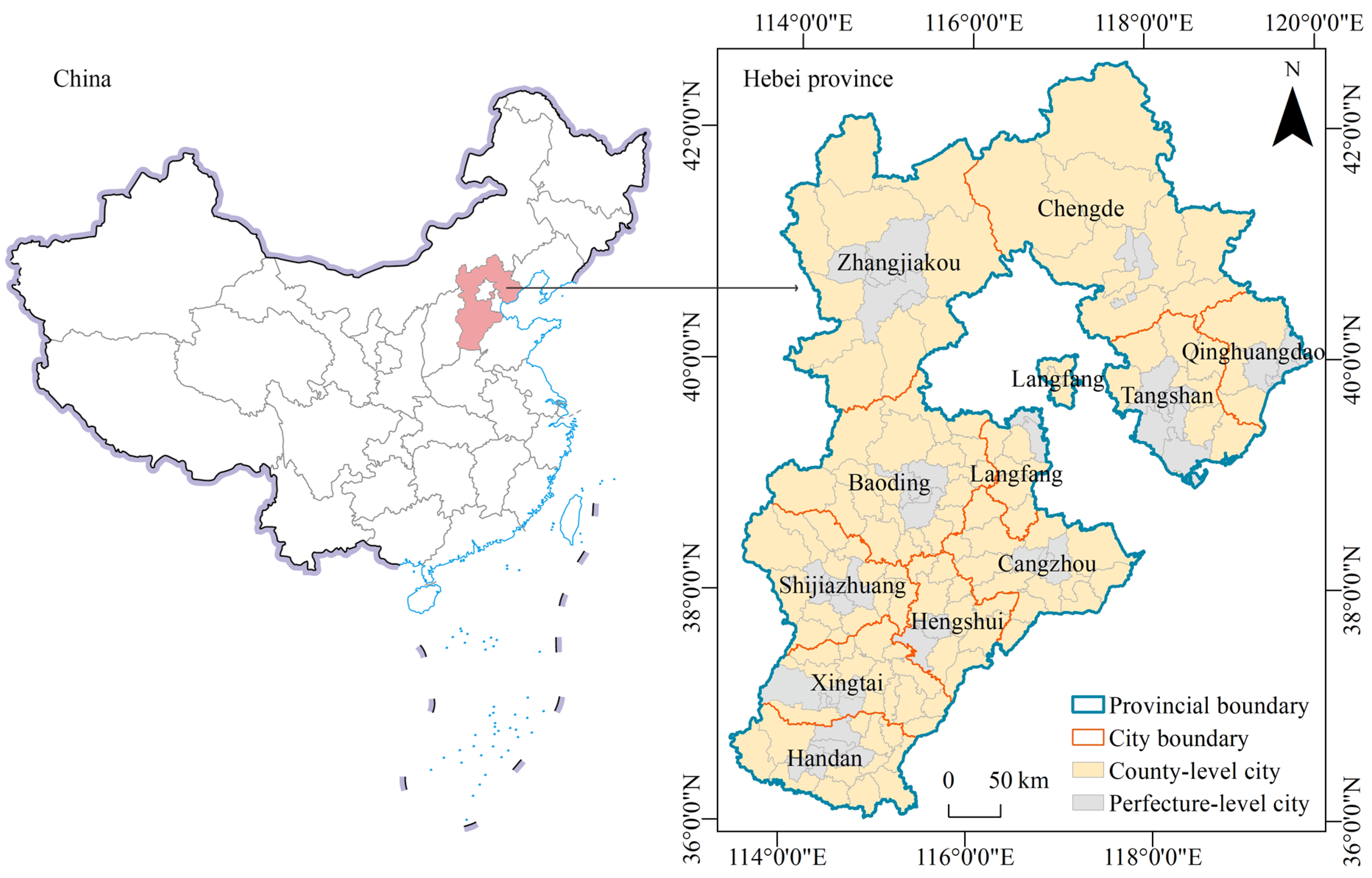
2.1. Study Area

The study area for this paper is 117 county-level cities in Hebei Province, China (Figure 1). Hebei Province is located in the Beijing–Tianjin–Hebei region, China’s “capital economic circle” and the largest and most dynamic economic region in northern China. This region has one of the most acute contradictions between economic development and the environment [56], as well as being one of the regions with the highest energy consumption intensity and the worst air pollution in country [57]. The carbon emissions of the Beijing–Tianjin–Hebei region were 601 million tons in 2020, and the carbon emissions of Hebei province were 366 million tons, which is 2.57 times and 4.00 times that of Beijing and Tianjin, respectively [58]. In the same year, road carbon emissions in the Beijing–Tianjin–Hebei region were 0.9 billion tons, with Hebei Province accounting for 0.6 billion tons. The future control of road carbon emissions in Hebei Province will be the focus of reductions in road carbon emissions in Beijing–Tianjin–Hebei region [59].

2.2. Influencing Factors Selection

In conjunction with existing relevant studies, four primary indicators from the perspective of the road traffic system are initially selected: highway network system, city road network system, public traffic system, and land use system of streets and transportation. Additionally, ten secondary indexes are further subdivided as shown in Table 1. All indicator data are counted in the city-wide area.
Highway transport emissions are the focus of carbon emissions in transportation, and improving the efficiency of highway transport organizations is a key initiative for reducing carbon emissions [65]. The density and connectivity of highway networks are the primary indicators of structural performance of highway networks [60]. Highway network density reflects the rationality of structure [60] and is an important indicator of highway network planning. The strength of traffic interconnection is reflected in highway network connectivity, which is an important indicator of structural performance [60].
The term “city road network” refers to the road system in the city’s built-up area. With the accelerated urbanization process, the demand for city road traffic is increasing, as are the resulting carbon emissions. City road traffic carbon emissions are becoming the focus of attention [66]. One of the many metrics currently used to study carbon emissions is city road network density [27,28,29], which reflects how dense the city road network is in urban areas. City road length is the total size of the city road network, and some studies have concluded that it has no significant effect on carbon emissions [26]; while others have suggested that it may have a negative effect on carbon emissions [61]. This paper will put it into the index system to see if some clearer conclusions can be drawn. To some extent, city road area per capita reflects the convenience of urban transportation, and some studies have suggested that it has a negative effect on urban carbon emissions [62], which is also considered in this paper for the reduction in carbon emissions.
Public traffic system has received more attention in the field of urban carbon emissions and is an important concern for lowering carbon emissions. The length of public transit routes and the density of public transit network reflect the scale and structure of the public traffic system. According to some studies, fewer bus miles traveled reduces carbon emissions [63], and network density has a negative effect on urban carbon emissions [30], making them the consideration for emission reductions.
The scale of the land use of street and transportation reflects the level of transportation’s facility supply. Some studies have concluded that it is positively correlated with carbon emissions [28,64], while others have concluded that the effect is not significant [27]. In this paper, three factors reflecting the total scale, per capita index, and percentage index are chosen for analysis to supplement the conclusion of the impact mechanism on urban carbon emissions.

2.3. Data Resources and Processing
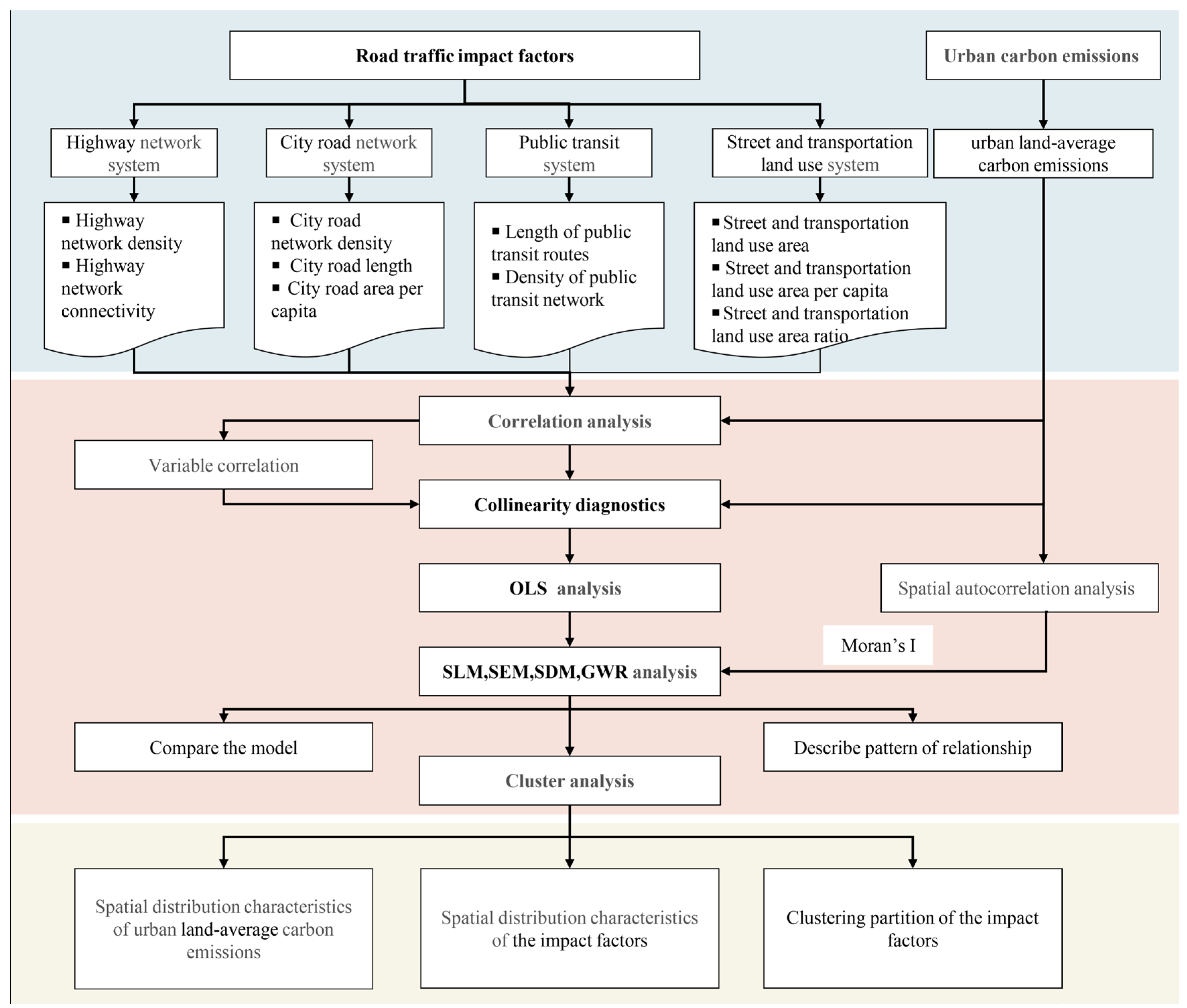
The total data of urban carbon emissions for this study were derived from the 2017 County-level CO2 Emissions in China from the China Carbon Emission Accounts and Datasets (CEADs) (https://www.ceads.net.cn, accessed on 27 May 2022). This dataset estimates CO2 emissions for 2735 counties in China from 1997 to 2017 using the swarm-optimized back propagation (PSO-BP) algorithm to unify the scale of DMSP/OLS and NPP/VIIRS satellite imagery. The dataset’s results were published in SCIENTIFIC DATA [67] and have received numerous citations [68,69,70,71].
Due to the large differences in the area of cities in the study area, this study shows the carbon emissions of each city in terms of urban land-average carbon emissions [72], and the values of land-average carbon emissions are calculated from CEADs data.
The China City Construction Statistical Yearbook [73] provides four impact factors: city road network density, city road length, city road area per capita, and street and transportation land use area. The relevant data from the China City Construction Statistical Yearbook are used to calculate highway network density, highway network connectivity, land use area per capita, and land use area ratio for streets and transportation methods. The length of public transit routes is obtained in part from each city’s statistical yearbook [74,75] and in part from data from Gaode Map (https://ditu.amap.com/, accessed on 2 June 2022), from which the density of public transit network is calculated.
The data of each index are shown in Figure 2.

2.4. Method

Figure 3 depicts the research framework for this study. To begin, impact indicators of road traffic are proposed, and key factors are identified using correlation analysis and collinearity diagnostics. Second, the spatial autocorrelation model is used to determine the spatial dependence of urban carbon emissions. The OLS, SLM, SEM, SDM, and GWR models are built to analyze the impacts of factors on urban carbon emissions by comparing the performance of the models and choosing the best model to determine the impact mechanism and spatial distribution characteristics. Finally, the main impact factors of each partition are clarified by clustering analysis, and a differentiated optimization strategy is proposed.

2.4.1. Correlation Analysis

Correlation analysis is used to determine the degree of similarity between the impact factors [36], and highly correlated indicators may result in information redundancy. The correlation coefficient is a statistical indicator that is used to indicate the closeness of relationships between variables. The calculation formula [76] is as follows:
r = i = 1 n X i   X ̲ Y i   Y ̲ i = 1 n X i   X ̲ 2 i = 1 n Y i   Y ̲ 2
Here, X and Y are the variables under consideration, and the absolute values of r are less than or equal to 1. If the value exceeds 0, it means that the two variables are positively correlated; otherwise, the two variables are negatively correlated. The stronger the correlation, the greater the absolute value of r.

2.4.2. Collinearity Diagnostics

When there are strongly correlated independent variables, the presence of multicollinearity must be determined by analyzing the variance inflation factors (VIF) of the metrics [36]. Multicollinearity can cause significant changes in the estimates of the regression coefficients, leading to model instability [77]. When the VIF value is greater than 5 to 10 or the conditional index is greater than 10 to 30 [78], multicollinearity exists and the variables must be excluded.

2.4.3. Spatial Autocorrelation Analysis

Spatial autocorrelation is used to examine the spatial correlation of variables, and spatial regression methods can only be used when the dependent variable is spatially correlated [36]. Moran’s I is the most commonly used indicator for investigating spatial autocorrelation. The calculation formula [79] is as follows:
I = n i = 1 n i = 1 n W i j x i x ¯ x j x ¯ i = 1 n i = 1 n W i j i = 1 n x i x ¯ 2
here, xi represents the observed value of city i, and Wij represents the spatial weight. Moran’s I has a value range from −1 to 1, with less than 0 indicating negative correlation, greater than 0 indicating positive correlation, and equal to 0 indicating that each spatial unit in the study area is independent of each other. If the value is closer to 1, it means that the spatial distribution of the study subjects has a greater aggregation effect. If the value is closer to −1, it means that there is a greater convergence in spatial distribution displayed by the study subjects.

2.4.4. Ordinary Least Squares (OLS)

The most commonly used linear regression models to explain the impacts of variables are ordinary least squares (OLS), which can analyze the degree of influence of the respective variables on the dependent variable at the global level. The calculation formula [80] is as follows:
y = β 0 + β 1 x 1 + β 2 x 2 + + β p x p + ε
Here, y is the dependent variable, and β 0 is the constant term.   β 1 , β 2 , and β p are the regression coefficients.   ε   is the stochastic error.
The goodness of fit is indicated by the regression result R2, and the closer the value is to 1, the better the fit.

2.4.5. Spatial Regression Model (SLM, SEM, SDM, and GWR)

When the dependent variable is spatially dependent, the spatial regression model is more useful. SLM, SEM, and SDM are global regression models. SLM estimates spatial effects by combining the spatial lags of the dependent variable [43,44]. SEM estimates spatial effects through spatial dependence in the error term [43,44]. SDM, on the other hand, estimates spatial effects using the dependent and independent variables’ spatial lags [45,46].
GWR is a local form of linear regression that can be used to model spatially varying relationships. GWR is capable of explaining local spatial relationships and spatial heterogeneity. The calculation formula [80] is as follows:
y i = β 0 u i , v i + k = 1 m β k u i , v i x i k + ε i
Here,   y i is the dependent variable’s value at position i,   x i k   is the independent variable’s value at position i,   u i , v i is location coefficient,   β 0 u i , v i is the intercept term, and β k u i , v i is the regression coefficient.

2.4.6. K-Means Cluster Analysis

Cluster analysis is the process of grouping data based on information about the indicators and their relationships found in the data, so that the indicators within and between groups exhibit homogeneity and heterogeneity, respectively [81]. The most commonly used cluster analysis method is k-means cluster [82], which automatically divides the data into k groups based on certain characteristics and iterates to determine the final groups based on the distance rule, which is based on the initial clustering centers selection. The F value is used to compare the intra-group and inter-group similarity of various grouping methods. The calculation formula [83] is as follows:
F = R 2 n c 1 1 R 2 n n c , R 2 = S S T S S E / S S T
Here, n is the number of data points, nc is the number of groups, SST is a statistic that measures component differences, and SSE is a statistic that measures similarity within groups.

3. Results and Analysis

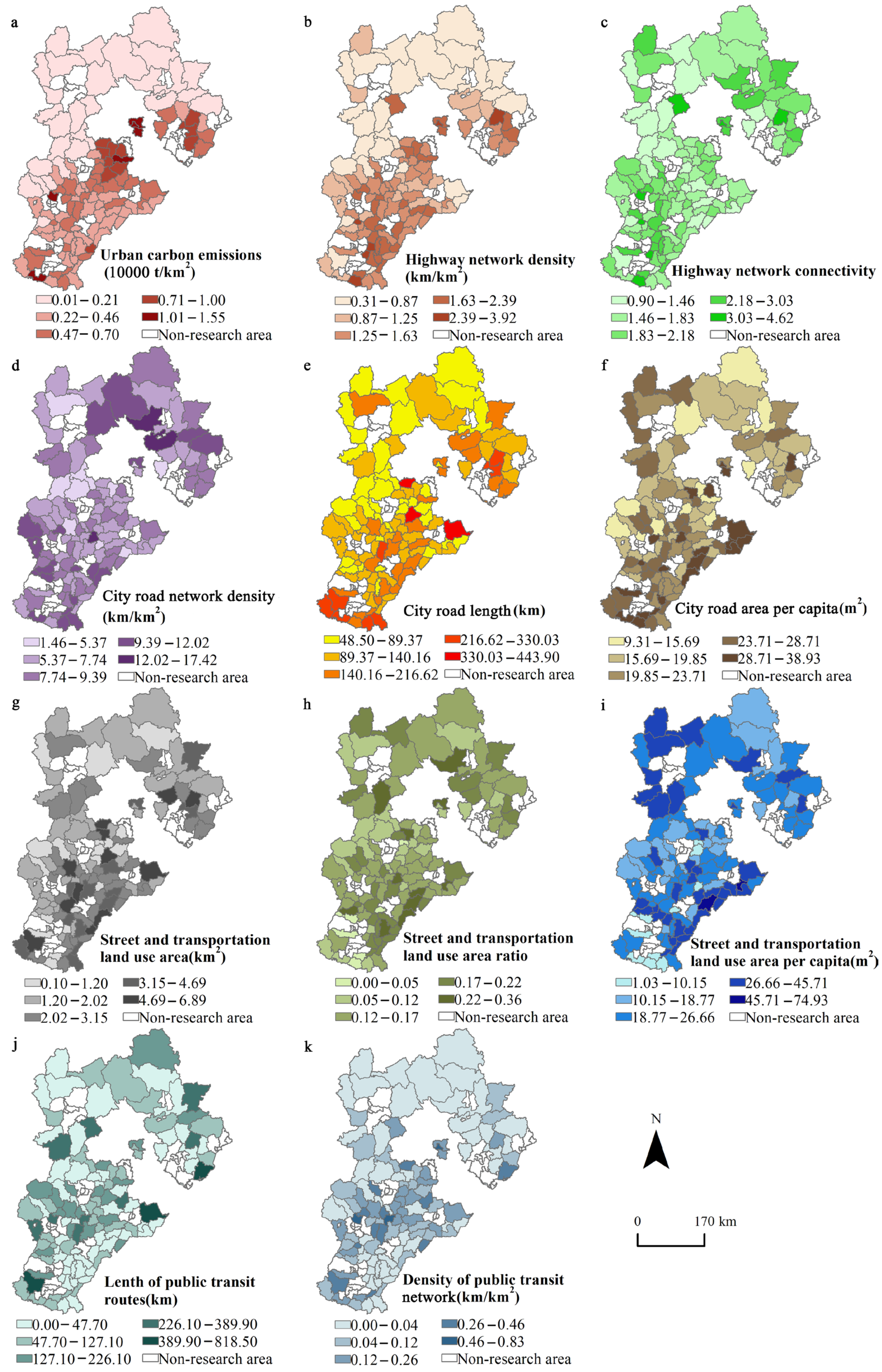
3.1. Spatial Distribution of Carbon Emissions

3.1.1. Overall Distribution of Land-Average Carbon Emissions

The overall distribution of land-average carbon emissions in the study area is uneven and shows obvious differences, with a decreasing trend from the southeast to the northwest. The highest value is 15,000 tons/km2 in Langfang, near Beijing, and the lowest value is 1000 tons/km2 in Chengde, in the north, with a 15-fold difference. Tangshan, Langfang, and Baoding in the ring around Beijing and Tianjin, and Shijiazhuang and Xingtai in the southwest, where heavy industry is more developed, have the highest land-average carbon emissions. These are the cities that must be prioritized for future efforts in reducing carbon emissions.

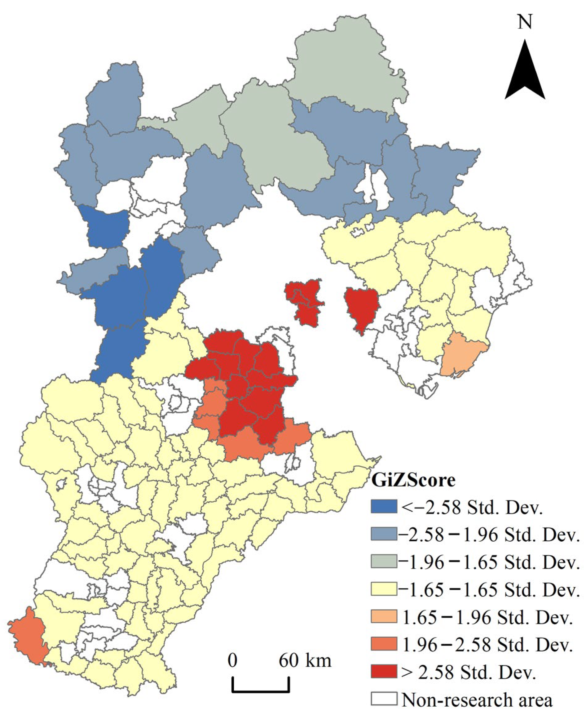
3.1.2. Spatial Autocorrelation of Land Average Carbon Emissions

Because the overall distribution of land-average carbon emissions shows obvious aggregation, a spatial autocorrelation analysis was performed. The results showed that Moran’s I was positive, indicating that carbon emissions were positively correlated. Meanwhile, the p value is 0.00, which is less than 0.05, and the Zscore is 8.5, which is greater than 2.58, indicating that there is some spatial clustering in urban land-average carbon emissions.
Further high/low clustering judgments were made, and the results revealed that the p value was 0.00, less than 0.05, and the Zscore was 7.19, greater than 2.58, indicating the presence of significant high clustering. The cold and hotspot analysis reveals that there are obvious cold and hotspot areas for urban land-average carbon emissions, with the hotspot areas primarily distributed around Beijing and Tianjin (Figure 4), indicating that the cities around Beijing and Tianjin are influenced by them, with correspondingly more frequent socio-economic activities and high energy consumption, and the cold spot areas primarily concentrated in northwestern Chengde and Zhangjiakou.

3.2. Impacts of Road Traffic on Carbon Emissions

3.2.1. Explanatory Variables Selection

The results of the correlation analysis (Figure 5) show that seven impact factors are significantly correlated with urban land-average carbon emissions. The correlation coefficients of three factors, namely, city road network density, land use area per capita, and land use area ratio of streets and transportation, did not pass the significance test with urban land-average carbon emissions and are thus excluded from the index.
At the same time, we discovered significant positive correlations with correlation coefficients greater than 0.7 between some influencing factors, including the highway network density and the highway network connectivity, the city road length and street and transportation land use area, the density of the public transit network, and the length of public transit routes. Because highly correlated variables can cause model instability, variables with low correlation with the dependent variable, such as highway network connectivity, street and transportation land use area, and length of public transit routes, were excluded.
The remaining four indicators were examined for collinearity, and the variance inflation factor (VIF) was less than five, indicating that there was no collinearity (Table 2). A preliminary regression analysis of these four indicators revealed that one of them failed the significance test, namely, the city road area per capita. This means that the indicator is not statistically significant and will be excluded from the following analysis.

3.2.2. Comparison of OLS, SLM, SEM, SDM, and GWR Models

Table 3 and Table 4 shows the results of the OLS, SLM, SEM, SDM, and GWR models, which were built by using three indicators: the highway network density, the city road length, and the density of public transit network.
The global OLS model had a lower R2 and a higher AICc, indicating that the spatial data’s explanatory power was insufficient. By creating spatial regression models SLM, SEM, and SDM, the model was enhanced, and it was discovered that R2 grew to approximately 0.65 and AICc decreased to approximately −40. This indicated that the spatial regression model had a better simulation performance, with the SLM model performing the best.
Despite being a better fit than OLS, SLM was unable to detect spatial differences in the explanatory variables within the study area. Therefore, a spatially non-smooth local model, GWR, was created. The results indicated that the GWR model is more effective than the global model at explaining the geographical non-stationarity of the data using spatially variable relationships, as shown by a higher R2 and a lower AICc than the SLM.
The distribution of the GWR model’s standardized residuals reveals that three cities are poorly fitted, while the remaining 114 sample cities are well fitted (Figure 6).
We find that the three impact variables have different effects on each city after further analyzing their regression coefficients. Figure 7 depicts the spatial distribution of the regression coefficients of the impact variables for each city in the study area. Overall, all of the impact factors exhibit significant piecewise spatial differentiation properties. The highway network density has a relatively large impact on the northern region. The northwestern region is more affected by the density of the public transit network. The southwest region is more affected by the city road length.
Specifically, the highway network density has a positive impact on the urban land-average carbon emissions, and the degree of impact decreases from north to south. The highest impact coefficients are found in Chengde, Zhangjiakou, Baoding, and Langfang around Beijing, while the lowest are found in Handan and Xingtai in the south.
The impact of public transit network density on the urban land-average carbon emissions is positive, and the impact value decreases from the southwest and northwest to the eastern region. Zhangjiakou in the northwest has the highest impact coefficient, while Chengde and Qinhuangdao in the eastern region have the lowest.
Except for one city, the city road length has a positive effect on the urban land-average carbon emissions, with the smallest impact coefficient of the three factors. From the southwest to the north, the magnitude of the impact decreases. The areas with the highest impact coefficients are concentrated in Shijiazhuang, Handan, and Xingtai in the southwest, while the smallest areas are concentrated in Chengde and Zhangjiakou in the northwest.

3.2.3. Cluster Partitioning

The results show that the study area can be divided into four characteristic categories of areas (Figure 8), and cities in the same category that exhibit strong spatial aggregation characteristics, using the K-mean clustering method to cluster the GWR coefficients of each impact factor. They can be divided into different types of dominant zones by horizontally contrasting the average value of each impact factor coefficient for urban land-average carbon emissions in four types of areas (Table 5).
Class I areas include 30 cities, the majority of which are located in northeast Tangshan, Qinhuangdao, Chengde, and Langfang, and Zhangjiakou in the central region. This area has the highest highway network density influence coefficient and can be considered a highway network dominant impact area.
Class II areas consist of four cities, the majority of which are located in Zhangjiakou in the northwest. This area has the highest impact factor on the density of the public transit network and can be considered the public transit-dominant impact area.
Class III areas consist of 35 cities, the majority of which are located in Shijiazhuang, Xingtai, and Handan in the southwest. This area has the highest impact factor on the city road length and can be considered the city road system’s dominant impact area.
Class IV areas contain 48 cities, which are mainly located in Hengshui, Cangzhou, and Baoding in the central region. The average coefficient of each influence factor in this area does not contain a maximum value and can be considered a multi-factor co-influence area.

4. Discussion

4.1. Differences in the Spatial Distribution of Land-Average Carbon Emissions

Using a spatial autocorrelation analysis, this study discovers significant spatial differences in the urban land-average carbon emissions in the study area, which is consistent with the findings of other studies [84]. The hotspot areas are primarily concentrated around Beijing and Tianjin, implying that Beijing and Tianjin affect the cities surrounding them, with correspondingly more frequent socioeconomic activities, a high population density, a relatively high passenger and freight traffic flow, and a high energy consumption, resulting in higher carbon emissions, as confirmed by a study on road traffic carbon emissions [59]. The cold spot area is primarily concentrated in northwestern Chengde and Zhangjiakou, which are far from Beijing, Tianjin, and heavy industrial areas, and they have low population density, low road density, relatively low intensity of socioeconomic activities, and thus, relatively low carbon emissions, which is also consistent with the current research on road traffic carbon emissions [59]. Therefore, the focus of low-carbon planning should be placed on hotspot areas.

4.2. The Impact of the Mechanisms of Road Traffic on Land-Average Carbon Emissions

This paper finds that the factors of road traffic affecting urban land-average carbon emissions are significantly spatially heterogeneous, with the dominant impact factors varying from city to city, requiring differentiated consideration when developing specific carbon reduction strategies. The highway network density has a relatively large impact on the northern region. The northwestern region is more affected by the density of the public transit network. The southwest areas are more affected by city road length.
Highway network density has a net positive effect on the urban land-average carbon emissions, which contradicts the findings of some previous studies [27]. The possible reason for this is that highways primarily transport passengers and freight traffic, and a higher highway network density means more highways per unit area and a longer total mileage, indicating that a greater traffic service capacity is provided and more traffic flows are carried, and the more carbon emissions are generated by passenger and freight vehicles, leading to increased highway carbon emissions. The inconsistency of urban development and traffic demand in different regions will result in different study conclusions.
City road length has a positive effect on the urban land-average carbon emissions, which contradicts the findings of some studies [26,61], but its impact is minor in comparison to the other two factors. The reason for this could be that the longer the road, the greater the service capacity, the greater the traffic volume it carries, and thus, the greater the carbon emissions generated. This is an indication that traffic demand in a county-level city has not yet reached saturation, and that continuous traffic demand is still increasing. This conclusion may not be applicable in large cities where traffic demand is close to or even exceeds saturation; thus, this may result in inconsistent findings across studies.
The density of the public transit network has a positive effect on the urban land-average carbon emissions, contrary to the popular belief that urban transit systems have a negative effect on urban carbon emissions. However, other studies have reached the different conclusions that an increase in the level of public transit services does not always result in a decrease in urban carbon emissions [85], because the majority of the increase in the proportion of public transit trips comes from bicycle and pedestrian traffic rather than car traffic, implying an increase in the total proportion of motorized trips and more energy consumption. This study also concludes a positive effect of the public transit system on urban carbon emissions, implying that increasing the level of public transit services serves to increase energy consumption rather than reduce urban carbon emissions. This means that the more developed public transportation is, the more attractive it is for the residents of towns to travel, and the greater the total transportation travel demand, thus resulting in an increase in carbon emissions from the means of public transportation. It also indicates that the proportion of the resident transportation mode in the study area has not changed from private to public, which deserves greater concern in low-carbon strategies.
Finally, all three secondary indicators have insignificant effects on the urban land-average carbon emissions in the indicator layer of land use for streets and transportation, which is consistent with the findings of some studies [27].

4.3. Suggestions for Road Traffic Planning

Firstly, in response to spatial differences in urban land-average carbon emissions, the focus of road transportation planning should be focused on hotspot areas around Beijing and Tianjin, particularly in regional urban planning, with transportation system optimization as a key planning tool.
Secondly, in response to the results of the road traffic indicator impact mechanism, low-carbon planning should prioritize the highway network system and the public transit system. The highway network system should focus on improving the efficiency of transport organization. In addition to the traditional planning of public transit corridors and station facilities, the focus of the public transit system should be placed on proposing initiatives to increase its attractiveness, such as increasing bus routes, scientifically establishing bus stops, opening special bus lines, and establishing intelligent public transit management systems, as they have the potential to reduce public transit travel time, improve efficiency, and increase the attractiveness of public transit travel in general, thereby reducing the proportion of private transportation travel, increasing the proportion of urban public transportation travel, and truly contributing to a reduction in urban carbon emissions.
Finally, in response to the results of the spatial heterogeneity of impact factors, traffic optimization strategies with different focuses should be developed according to the four categories of areas with different characteristics and the clustering partition. Class I areas should focus on improving the efficiency of highway transport organizations. Class II areas should focus on optimizing the public transit network and improving the attractiveness of public transit in order to shift the proportion of private car trips and reduce the overall traffic carbon emissions. Class III areas should prioritize reducing traffic congestion on city roads and increasing the proportion of the green transportation trips. Class IV areas are multi-factor areas that are relatively influenced by the public transit system, and they should focus on improving the attractiveness of public transit in the future.

4.4. Limitations and Future Prospects

This paper establishes road traffic indicators that affect the urban land-average carbon emissions, delves into the impact mechanisms of each indicator on carbon emissions, and offers recommendations for low-carbon development in urban transportation planning. There are some limitations and potential future avenues for further optimization in this study.
First, the carbon emissions data for the cities in this paper’s research region are obtained from open databases, and more accurate carbon emissions data values will be available in the future.
Second, the research area of this paper is the key metropolitan area in northern China; other key metropolitan areas, such as the central Yangtze River Delta and the southern Pearl River Delta, may have different research findings due to inconsistent urban development levels, and the fact that more research and optimization strategies for different regions are required.
Third, this research was only conducted in a single time cross-section, and if the researchers want to understand the changes in the impact of each factor index on urban carbon emissions more deeply, they should collect and compare data from multiple time cross-sections and should conduct more in-depth research in this field in the future.
Finally, in the new data environment, more new technical methods may emerge that can be used to conduct more in-depth research in the future.

5. Conclusions

This study establishes comprehensive road traffic indicators covering four aspects by constructing a sample database of 117 county-level cities: the highway network system, the city road network system, the public transit system, and the land use area system of streets and transportation. The impacts of road traffic indicators on the urban land-average carbon emissions are investigated, and distinct transportation optimization strategies are proposed. From the perspective of transportation, the methodology and fields of research on urban carbon emissions are supplemented. The research findings can assist policymakers in developing more targeted carbon reduction policies, provide useful references for urban planning practitioners in developing planning schemes, and serve as a foundation for economic sectors in developing investment strategies.
The following are the main conclusions:
  • The distribution of urban land-average carbon emissions has obvious spatial differences, with hotspot areas primarily located around Beijing and Tianjin, which should be prioritized in low-carbon work.
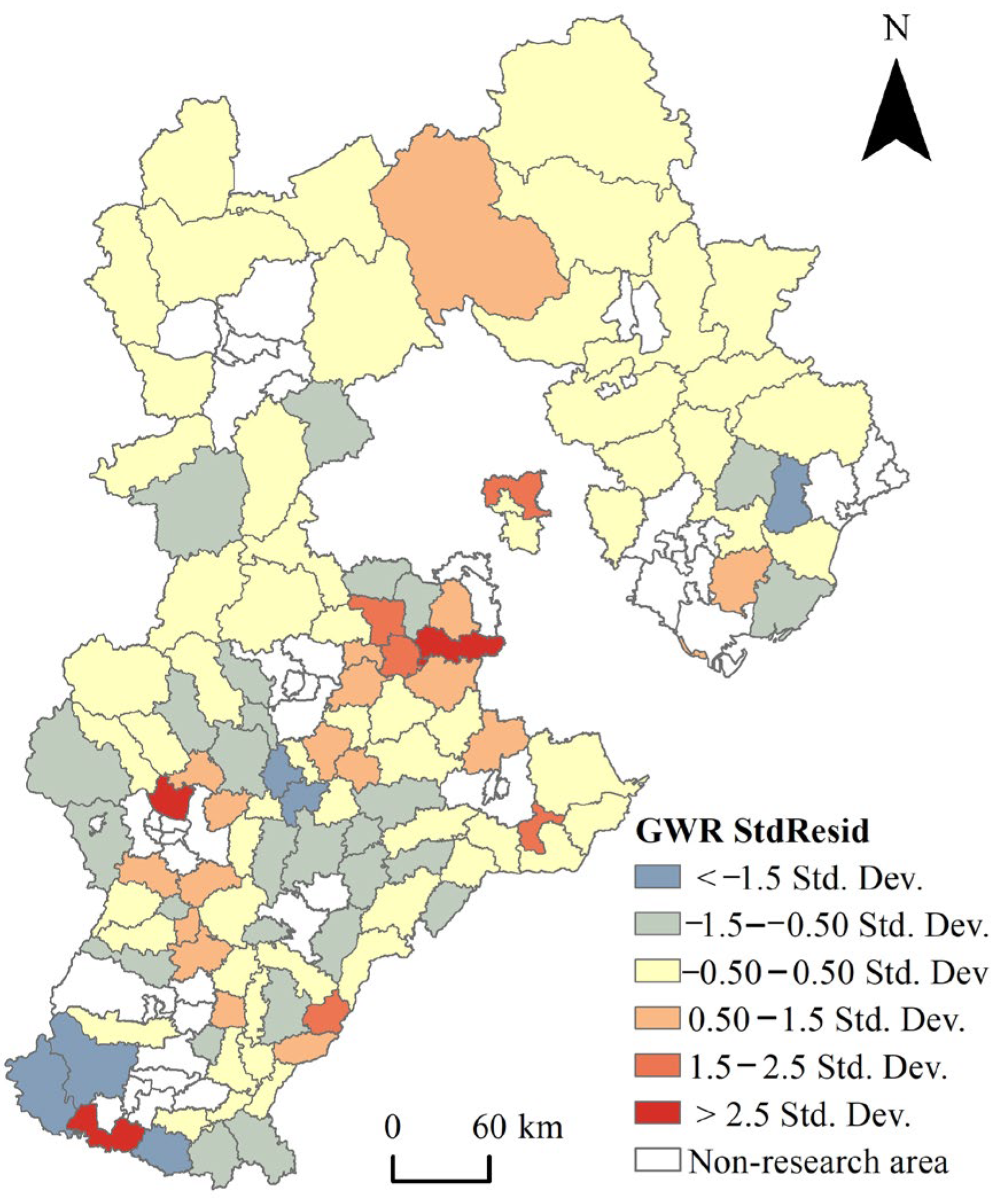
  • The global models (OLS, SLM, SEM, and SDM) and the local model (GWR) were built to analyze the impact mechanism, and it was discovered that the GWR model has a higher R2 value and a smaller AICc value, which has a better model performance.
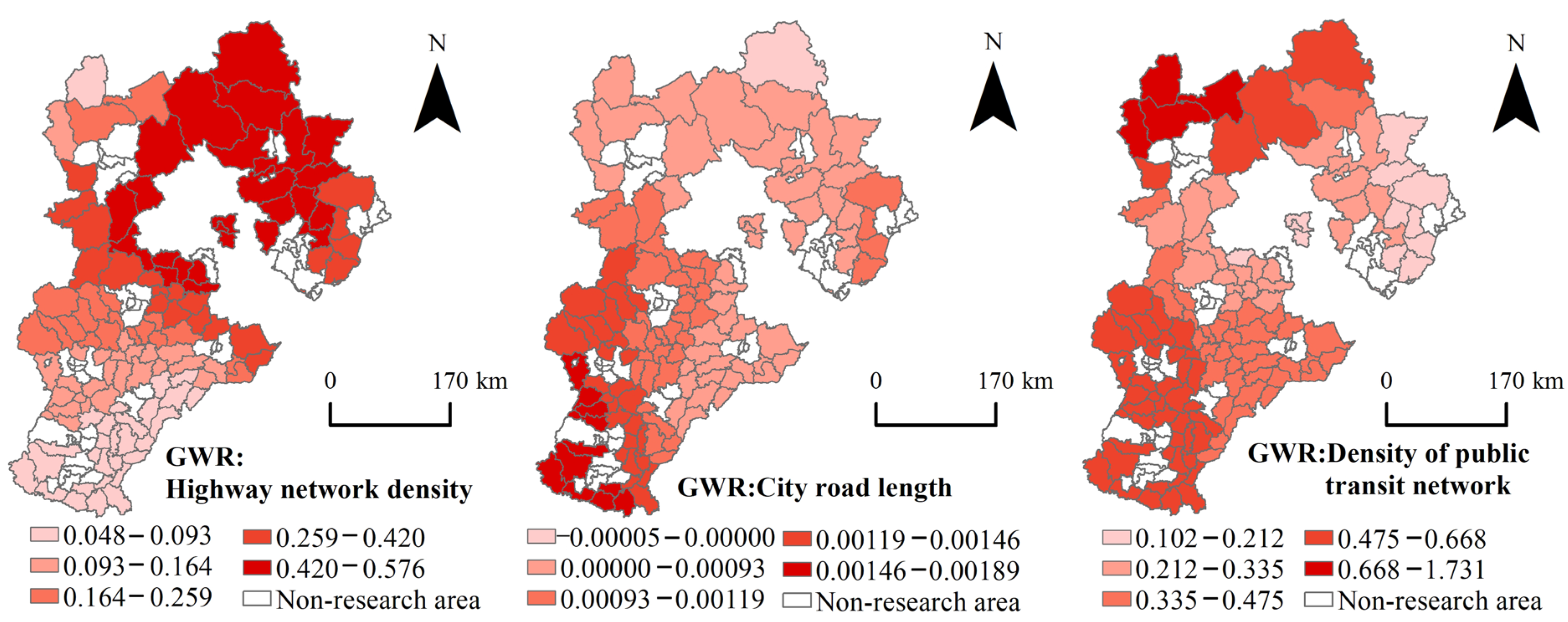
  • The three indicators of highway network density, city road length, and density of public transit network all have a significant effect on urban land-average carbon emissions, but the land use area system of streets and transportation has no effect. The emphasis should be on the highway network and public transit systems, particularly concerning initiatives to improve the efficiency of highway transportation organization and increase the proportion of public transportation trips.
  • The GWR model’s results show that there is significant piecewise spatial differentiation in the impact of the three factors on the urban land-average carbon emissions. The highway network density has a relatively large impact on the northern region. The northwestern region is more affected by the density of the public transit network. The southwest are more affected by the city road length.
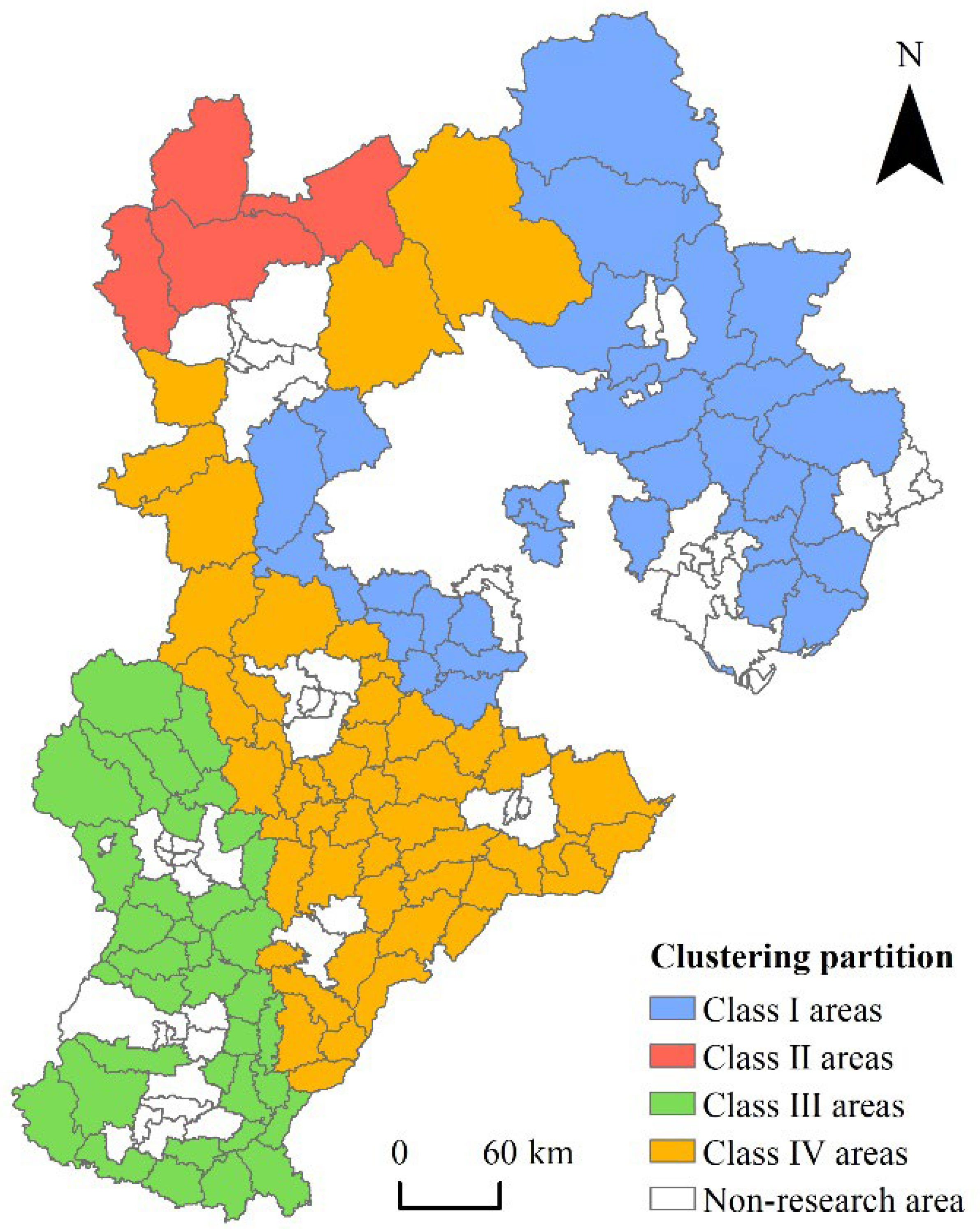
  • By means of clustering, the study area was divided into four categories of dominant areas of different impact factors, and targeted traffic optimization recommendations were made. Class I areas are highway network dominant impact areas, where the focus should be placed on improving the efficiency of highway transport organization. Class II areas are public transit dominant impact areas, where the focus should be on optimizing the public transit network and improving the attractiveness of public transit. Class III areas are city road network dominant impact areas, where the focus should be on reducing traffic congestion on city roads and increasing the proportion of the green transportation trips. Class IV areas are multi-factor areas and they should be relatively focused on improving the attractiveness of public transit.

Author Contributions

Conceptualization, H.L., A.N. and S.Z.; methodology, H.L. and A.N.; software, H.L. and A.N.; validation, H.L., J.Z. and S.Z.; formal analysis, H.L.; investigation, H.L.; resources, H.L. and S.Z.; data curation, H.L.; writing—original draft preparation, H.L. and A.N.; writing—review and editing, H.L., S.Z., A.N. and S.Z.; visualization, H.L. and A.N.; supervision, J.Z. and S.Z.; project administration, S.Z. and J.Z.; funding acquisition, S.Z. All authors have read and agreed to the published version of the manuscript.

Funding

This research was funded by the National Natural Science Foundation of China (NSFC) (grant number 52078320).

Institutional Review Board Statement

Not applicable.

Informed Consent Statement

Not applicable.

Data Availability Statement

The data presented in this study are available on request from the corresponding author.

Acknowledgments

The authors would like to thank the reviewers for their expertise and valuable input.

Conflicts of Interest

The authors declare no conflict of interest.

References

  1. Urban, M.C. Accelerating extinction risk from climate change. Science 2015, 348, 571–573. [Google Scholar] [CrossRef] [Green Version]
  2. IPCC. Global Warming of 1.5 °C: IPCC Special Report on Impacts of Global Warming of 1.5 °C above Pre-industrial Levels in Context of Strengthening Response to Climate Change, Sustainable Development, and Efforts to Eradicate Poverty; Cambridge University Press: Cambridge, UK, 2022. [Google Scholar]
  3. Maris, G.; Flouros, F. The Green Deal, National Energy and Climate Plans in Europe: Member States’ Compliance and Strategies. Adm. Sci. 2021, 11, 75. [Google Scholar] [CrossRef]
  4. Fragkos, P.; van Soest, H.L.; Schaeffer, R.; Reedman, L.; Köberle, A.C.; Macaluso, N.; Evangelopoulou, S.; De Vita, A.; Sha, F.; Qimin, C.; et al. Energy system transitions and low-carbon pathways in Australia, Brazil, Canada, China, EU-28, India, Indonesia, Japan, Republic of Korea, Russia and the United States. Energy 2021, 216, 119385. [Google Scholar] [CrossRef]
  5. Roelfsema, M.; van Soest, H.L.; Harmsen, M.; van Vuuren, D.P.; Bertram, C.; Elzen, M.D.; Höhne, N.; Iacobuta, G.; Krey, V.; Kriegler, E.; et al. Taking stock of national climate policies to evaluate implementation of the Paris Agreement. Nat. Commun. 2020, 11, 2096. [Google Scholar] [CrossRef]
  6. IEA. Net Zero by 2050, License: CC BY 4.0. 2021. Available online: https://www.iea.org/reports/net-zero-by-2050 (accessed on 20 December 2022).
  7. Lamb, W.F.; Wiedmann, T.; Pongratz, J.; Andrew, R.; Crippa, M.; Olivier, J.G.J.; Wiedenhofer, D.; Mattioli, G.; Al Khourdajie, A.; House, J.; et al. A review of trends and drivers of greenhouse gas emissions by sector from 1990 to 2018. Environ. Res. Lett. 2021, 16, 073005. [Google Scholar] [CrossRef]
  8. IEA. An Energy Sector Roadmap to Carbon Neutrality in China, IEA, License: CC BY 4.0. 2021. Available online: https://www.iea.org/reports/an-energy-sector-roadmap-to-carbon-neutrality-in-china (accessed on 28 December 2022).
  9. Muñiz, I.; Garcia-López, M. Urban form and spatial structure as determinants of the ecological footprint of commuting. Transp. Res. Part D Transp. Environ. 2019, 67, 334–350. [Google Scholar] [CrossRef]
  10. Hong, S.; Hui, E.C.-M.; Lin, Y. Relationship between urban spatial structure and carbon emissions: A literature review. Ecol. Indic. 2022, 144, 109456. [Google Scholar] [CrossRef]
  11. Li, C.; Zhang, L.; Gu, Q.; Guo, J.; Huang, Y. Spatio-Temporal Differentiation Characteristics and Urbanization Factors of Urban Household Carbon Emissions in China. Int. J. Environ. Res. Public Health 2022, 19, 4451. [Google Scholar] [CrossRef] [PubMed]
  12. Yu, X.; Wu, Z.; Zheng, H.; Li, M.; Tan, T. How urban agglomeration improve the emission efficiency? A spatial econometric analysis of the Yangtze River Delta urban agglomeration in China. J. Environ. Manag. 2020, 260, 110061. [Google Scholar] [CrossRef]
  13. Ou, J.; Liu, X.; Li, X.; Chen, Y. Quantifying the relationship between urban forms and carbon emissions using panel data analysis. Landsc. Ecol. 2013, 28, 1889–1907. [Google Scholar] [CrossRef]
  14. Creutzig, F.; Baiocchi, G.; Bierkandt, R.; Pichler, P.-P.; Seto, K.C. Global typology of urban energy use and potentials for an urbanization mitigation wedge. Proc. Natl. Acad. Sci. USA 2015, 112, 6283–6288. [Google Scholar] [CrossRef] [PubMed] [Green Version]
  15. Underwood, A.; Fremstad, A. Does sharing backfire? A decomposition of household and urban economies in CO2 emissions. Energy Policy 2018, 123, 404–413. [Google Scholar] [CrossRef]
  16. Waygood, E.; Sun, Y.; Susilo, Y.O. Transportation carbon dioxide emissions by built environment and family lifecycle: Case study of the Osaka metropolitan area. Transp. Res. Part D Transp. Environ. 2014, 31, 176–188. [Google Scholar] [CrossRef]
  17. Antequera, P.D.; Pacheco, J.D.; Díez, A.L.; Herrera, C.B. Tourism, Transport and Climate Change: The Carbon Footprint of International Air Traffic on Islands. Sustainability 2021, 13, 1795. [Google Scholar] [CrossRef]
  18. Duffy, A. Land use planning in Ireland—A life cycle energy analysis of recent residential development in the Greater Dublin Area. Int. J. Life Cycle Assess. 2009, 14, 268–277. [Google Scholar] [CrossRef] [Green Version]
  19. Hussain, Z.; Khan, M.K.; Xia, Z. Investigating the role of green transport, environmental taxes and expenditures in mitigating the transport CO2 emissions. Transp. Lett. 2022, 14, 1–11. [Google Scholar] [CrossRef]
  20. Sharifi, A. Co-benefits and synergies between urban climate change mitigation and adaptation measures: A literature review. Sci. Total. Environ. 2021, 750, 141642. [Google Scholar] [CrossRef] [PubMed]
  21. Sun, C.; Zhang, Y.; Ma, W.; Wu, R.; Wang, S. The Impacts of Urban Form on Carbon Emissions: A Comprehensive Review. Land 2022, 11, 1430. [Google Scholar] [CrossRef]
  22. Li, H.; Luo, N. Will improvements in transportation infrastructure help reduce urban carbon emissions?—Motor vehicles as transmission channels. Environ. Sci. Pollut. Res. 2022, 29, 38175–38185. [Google Scholar] [CrossRef] [PubMed]
  23. Pang, M.B.; Wei, L.Y. Systems Engineering and Transportation; Tianjin People’s Publishing House: Tianjin, China, 2004; pp. 20–24. [Google Scholar]
  24. Aditjandra, P.T.; Mulley, C.; Nelson, J.D. The influence of neighbourhood design on travel behaviour: Empirical evidence from North East England. Transp. Policy 2013, 26, 54–65. [Google Scholar] [CrossRef]
  25. Harari, M. Cities in Bad Shape: Urban Geometry in India. Am. Econ. Rev. 2020, 110, 2377–2421. [Google Scholar] [CrossRef]
  26. Kang, J.-G.; Oh, H.-U. Factors affecting vehicles’ carbon emission in road networks. Transp. A Transp. Sci. 2016, 12, 736–750. [Google Scholar] [CrossRef]
  27. Zhang, H.; Zhang, J.X.; Wang, R.; Ya, M.; Peng, J.Y. The mechanism of the built environment of small cities on the carbon emissions of residents’ travel and transportation. Urban Issues 2020, 4–10. [Google Scholar] [CrossRef]
  28. Cao, X.; Yang, W. Examining the effects of the built environment and residential self-selection on commuting trips and the related CO 2 emissions: An empirical study in Guangzhou, China. Transp. Res. Part D Transp. Environ. 2017, 52, 480–494. [Google Scholar] [CrossRef]
  29. Hou, Q.; Zhang, X.; Li, B.; Zhang, X.; Wang, W. Identification of low-carbon travel block based on GIS hotspot analysis using spatial distribution learning algorithm. Neural Comput. Appl. 2019, 31, 4703–4713. [Google Scholar] [CrossRef]
  30. Zhang, H.; Yu, D.Y.; Wang, R.; Sheng, M.J. China’s Provincial Low Carbon Planning Strategy Based on Carbon Emission Features. Build. Energy Effic. 2020, 48, 126–132. [Google Scholar] [CrossRef]
  31. Li, T.; Wu, J.; Dang, A.; Liao, L.; Xu, M. Emission pattern mining based on taxi trajectory data in Beijing. J. Clean. Prod. 2019, 206, 688–700. [Google Scholar] [CrossRef]
  32. Lee, S.; Lee, B. The influence of urban form on GHG emissions in the U.S. household sector. Energy Policy 2014, 68, 534–549. [Google Scholar] [CrossRef]
  33. Ma, J.; Liu, Z.; Chai, Y. The impact of urban form on CO2 emission from work and non-work trips: The case of Beijing, China. Habitat Int. 2015, 47, 1–10. [Google Scholar] [CrossRef]
  34. Kissinger, M.; Reznik, A. Detailed urban analysis of commute-related GHG emissions to guide urban mitigation measures. Environ. Impact Assess. Rev. 2019, 76, 26–35. [Google Scholar] [CrossRef]
  35. Li, H.; Strauss, J.; Liu, L. A Panel Investigation of High-Speed Rail (HSR) and Urban Transport on China’s Carbon Footprint. Sustainability 2019, 11, 2011. [Google Scholar] [CrossRef] [Green Version]
  36. Zheng, S.; Huang, Y.; Sun, Y. Effects of Urban Form on Carbon Emissions in China: Implications for Low-Carbon Urban Planning. Land 2022, 11, 1343. [Google Scholar] [CrossRef]
  37. Ye, H.; Qiu, Q.; Zhang, G.; Lin, T.; Li, X. Effects of natural environment on urban household energy usage carbon emissions. Energy Build. 2013, 65, 113–118. [Google Scholar] [CrossRef]
  38. Yi, Y.; Wang, Y.; Li, Y.; Qi, J. Impact of urban density on carbon emissions in China. Appl. Econ. 2021, 53, 6153–6165. [Google Scholar] [CrossRef]
  39. Zhu, C.; Du, W. A Research on Driving Factors of Carbon Emissions of Road Transportation Industry in Six Asia-Pacific Countries Based on the LMDI Decomposition Method. Energies 2019, 12, 4152. [Google Scholar] [CrossRef] [Green Version]
  40. Jiang, R.; Wu, P.; Wu, C. Driving Factors behind Energy-Related Carbon Emissions in the U.S. Road Transport Sector: A Decomposition Analysis. Int. J. Environ. Res. Public Health 2022, 19, 2321. [Google Scholar] [CrossRef] [PubMed]
  41. Saboori, B.; Sapri, M.; bin Baba, M. Economic growth, energy consumption and CO2 emissions in OECD (Organization for Economic Co-operation and Development)’s transport sector: A fully modified bi-directional relationship approach. Energy 2014, 66, 150–161. [Google Scholar] [CrossRef]
  42. Anselin, L. Spatial Econometrics: Methods and Models; Kluwer Academic Publishers: Dordrecht, The Netherlands, 1988; pp. 137–168. [Google Scholar]
  43. Sannigrahi, S.; Pilla, F.; Basu, B.; Basu, A.S.; Molter, A. Examining the association between socio-demographic composition and COVID-19 fatalities in the European region using spatial regression approach. Sustain. Cities Soc. 2020, 62, 102418. [Google Scholar] [CrossRef] [PubMed]
  44. Mansour, S.; Al Kindi, A.; Al-Said, A.; Al-Said, A.; Atkinson, P. Sociodemographic determinants of COVID-19 incidence rates in Oman: Geospatial modelling using multiscale geographically weighted regression (MGWR). Sustain. Cities Soc. 2021, 65, 102627. [Google Scholar] [CrossRef]
  45. Majeed, M.T.; Mazhar, M. An empirical analysis of output volatility and environmental degradation: A spatial panel data approach. Environ. Sustain. Indic. 2021, 10, 100104. [Google Scholar] [CrossRef]
  46. Wang, S.; Chen, Y.; Huang, J.; Chen, N.; Lu, Y. Macrolevel Traffic Crash Analysis: A Spatial Econometric Model Approach. Math. Probl. Eng. 2019, 2019, 5306247. [Google Scholar] [CrossRef] [Green Version]
  47. Wei, L.; Liu, Z. Spatial heterogeneity of demographic structure effects on urban carbon emissions. Environ. Impact Assess. Rev. 2022, 95, 106790. [Google Scholar] [CrossRef]
  48. Cheng, Y.-H.; Chang, Y.-H.; Lu, I.J. Urban transportation energy and carbon dioxide emission reduction strategies. Appl. Energy 2015, 157, 953–973. [Google Scholar] [CrossRef] [PubMed]
  49. Paladugula, A.L.; Kholod, N.; Chaturvedi, V.; Ghosh, P.P.; Pal, S.; Clarke, L.; Evans, M.; Kyle, P.; Koti, P.N.; Parikh, K.; et al. A multi-model assessment of energy and emissions for India’s transportation sector through 2050. Energy Policy 2018, 116, 10–18. [Google Scholar] [CrossRef]
  50. Adams, S.; Boateng, E.; Acheampong, A.O. Transport energy consumption and environmental quality: Does urbanization matter? Sci. Total Environ. 2020, 744, 140617. [Google Scholar] [CrossRef]
  51. Amin, A.; Altinoz, B.; Dogan, E. Analyzing the determinants of carbon emissions from transportation in European countries: The role of renewable energy and urbanization. Clean Technol. Environ. Policy 2020, 22, 1725–1734. [Google Scholar] [CrossRef]
  52. Zhu, W.; Ding, C.; Cao, X. Built environment effects on fuel consumption of driving to work: Insights from on-board diagnostics data of personal vehicles. Transp. Res. Part D Transp. Environ. 2019, 67, 565–575. [Google Scholar] [CrossRef]
  53. Keuken, M.; Jonkers, S.; Verhagen, H.; Perez, L.; Trüeb, S.; Okkerse, W.-J.; Liu, J.; Pan, X.; Zheng, L.; Wang, H.; et al. Impact on air quality of measures to reduce CO2 emissions from road traffic in Basel, Rotterdam, Xi’an and Suzhou. Atmos. Environ. 2014, 98, 434–441. [Google Scholar] [CrossRef]
  54. He, D.; Meng, F.; Wang, M.Q.; He, K. Impacts of Urban Transportation Mode Split on CO2 Emissions in Jinan, China. Energies 2011, 4, 685–699. [Google Scholar] [CrossRef] [Green Version]
  55. Su, Y.; Wu, J.; Ciais, P.; Zheng, B.; Wang, Y.; Chen, X.; Li, X.; Li, Y.; Wang, Y.; Wang, C.; et al. Differential impacts of urbanization characteristics on city-level carbon emissions from passenger transport on road: Evidence from 360 cities in China. Build. Environ. 2022, 219, 109165. [Google Scholar] [CrossRef]
  56. Zang, H.K.; Yang, W.S.; Zhang, J.; Wu, P.C.; Cao, L.B.; Xu, Y. Research on carbon dioxide emissions peaking in Beijing-Tianjin-Hebei city agglomeration. Environ. Eng. 2020, 38, 19–24. [Google Scholar] [CrossRef]
  57. Zhang, W.; Zhang, J.; Wang, F.; Jiang, H.Q.; Wang, J.N.; Jiang, L. Spatial Agglomeration of Industrial Air Pollutant Emission in Beijing-Tianjin-Hebei Region. Urban Dev. Stud. 2017, 24, 81–87. [Google Scholar] [CrossRef]
  58. Ye, T.L.; Li, G.L. Annual Report on Beijing-Tianjin-Hebei Metropolitan Region Development (2022); Social Science Literature Press: Beijing, China, 2022; pp. 86–123. [Google Scholar]
  59. Liu, H.; Li, Y.X.; Yu, F.J.; Lv, C.; Yang, N.; Liu, Z.L.; Zhao, M. Evolution and spatial distribution of road carbon emissions in Beijing-Tianjin-Hebei region. China Environ. Sci. 2022, 1–12. [Google Scholar] [CrossRef]
  60. Shi, Y.Z.; Chen, X.W.; Liu, S.M. Technical Evaluation indicator and Standard in Highway Network Planning. China J. Highw. Transp. 1995, 8, 120–124. [Google Scholar] [CrossRef]
  61. Ge, Q.Y.; Xu, Y.N.; Qiu, R.Z.; Hu, X.S.; Zhang, Y.Y.; Liu, N.C.; Zhang, L.Y. Scenario simulation of urban passenger transportation carbon reduction based on system dynamics. Clim. Change Res. 2022, 1–16. [Google Scholar] [CrossRef]
  62. Chen, Z.Q.; Lin, X.B.; Li, L.; Li, G.C. Does Urban Spatial Morphology Affect Carbon Emission?: A Study Based on 110 Prefectural Cities. Ecol. Econ. 2016, 32, 22–26. [Google Scholar] [CrossRef]
  63. Tong, K.K.; Ma, K.M. Significant impact of job-housing distance on carbon emissions from transport: A scenario analysis. Acta Ecol. Sin. 2012, 32, 2975–2984. [Google Scholar] [CrossRef] [Green Version]
  64. Pasha, M.; Rifaat, S.M.; Tay, R.; De Barros, A. Effects of street pattern, traffic, road infrastructure, socioeconomic and demographic characteristics on public transit ridership. KSCE J. Civ. Eng. 2016, 20, 1017–1022. [Google Scholar] [CrossRef]
  65. Li, X.; Tan, X.; Wu, R.; Xu, H.; Zhong, Z.; Li, Y.; Zheng, C.; Wang, R.; Qiao, Y. Paths for Carbon Peak and Carbon Neutrality in Transport Sector in China. Chin. J. Eng. Sci. 2021, 23, 15–21. [Google Scholar] [CrossRef]
  66. Zhang, T.X. Research on China’s Urban Road Transport Carbon Emissions under Urbanization Process. China Popul. Resour. Environ. 2012, 22, 3–9. [Google Scholar] [CrossRef]
  67. Chen, J.; Gao, M.; Cheng, S.; Hou, W.; Song, M.; Liu, X.; Liu, Y.; Shan, Y. County-level CO2 emissions and sequestration in China during 1997–2017. Sci. Data 2020, 7, 391. [Google Scholar] [CrossRef]
  68. Zhang, S.; Bai, X.; Zhao, C.; Tan, Q.; Luo, G.; Wu, L.; Xi, H.; Li, C.; Chen, F.; Ran, C.; et al. China’s carbon budget inventory from 1997 to 2017 and its challenges to achieving carbon neutral strategies. J. Clean. Prod. 2022, 347, 130966. [Google Scholar] [CrossRef]
  69. Zhang, W.; Liu, X.; Wang, D.; Zhou, J. Digital economy and carbon emission performance: Evidence at China’s city level. Energy Policy 2022, 165, 112927. [Google Scholar] [CrossRef]
  70. Dong, Z.; Xia, C.; Fang, K.; Zhang, W. Effect of the carbon emissions trading policy on the co-benefits of carbon emissions reduction and air pollution control. Energy Policy 2022, 165, 112998. [Google Scholar] [CrossRef]
  71. Huo, W.; Qi, J.; Yang, T.; Liu, J.; Liu, M.; Zhou, Z. Effects of China’s pilot low-carbon city policy on carbon emission reduction: A quasi-natural experiment based on satellite data. Technol. Forecast. Soc. Chang. 2022, 175, 121422. [Google Scholar] [CrossRef]
  72. Zhang, J.; Chen, H.; Liu, D.; Shi, Q.Q.; Geng, T.W. The spatial and temporal variation and influencing factors of land use carbon emissions at county scale. J. Northwest Univ. 2022, 52, 21–31. [Google Scholar] [CrossRef]
  73. Ministry of Housing and Urban-Rural Development of the People’s Republic of China. China Urban Construction Statistical Yearbook 2017; China Statistics Press: Beijing, China, 2018; pp. 45–83. [Google Scholar]
  74. DaChang Bureau of Statistics. DaChang Yearbook 2017; China Communist Party History Press: Beijing, China, 2018; pp. 183–190. [Google Scholar]
  75. ZhaoXian Bureau of Statistics. ZhaoXian Yearbook 2017; Hebei Peoples Publishing House: Shi Jiazhuang, China, 2018; pp. 240–246. [Google Scholar]
  76. Gejingting, X.; Ruiqiong, J.; Wei, W.; Libao, J.; Zhenjun, Y. Correlation analysis and causal analysis in the era of big data. IOP Conf. Ser. Mater. Sci. Eng. 2019, 563, 42032. [Google Scholar] [CrossRef]
  77. Lavery, M.R.; Acharya, P.; Sivo, S.A.; Xu, L. Number of predictors and multicollinearity: What are their effects on error and bias in regression? Commun. Stat. Simul. Comput. 2018, 48, 27–38. [Google Scholar] [CrossRef]
  78. Kim, J.H. Multicollinearity and misleading statistical results. Korean J. Anesthesiol. 2019, 72, 558–569. [Google Scholar] [CrossRef] [PubMed] [Green Version]
  79. Hu, X.; Ma, C.; Huang, P.; Guo, X. Ecological vulnerability assessment based on AHP-PSR method and analysis of its single parameter sensitivity and spatial autocorrelation for ecological protection—A case of Weifang City, China. Ecol. Indic. 2021, 125, 107464. [Google Scholar] [CrossRef]
  80. Park, J.; Choi, B.; Lee, J. Spatial Distribution Characteristics of Species Diversity Using Geographically Weighted Regression Model. Sens. Mater. 2019, 31, 3197. [Google Scholar] [CrossRef] [Green Version]
  81. Han, C.F.; Song, F.L.; Teng, M.M. Temporal and Spatial Dynamic Characteristics, Spatial Clustering and Governance Strategies of Carbon Emissions in the Yangtze River Delta. East China Econ. Manag. 2022, 36, 24–33. [Google Scholar] [CrossRef]
  82. Sinaga, K.P.; Yang, M.-S. Unsupervised K-Means Clustering Algorithm. IEEE Access 2020, 8, 80716–80727. [Google Scholar] [CrossRef]
  83. Gu, H.Y.; Meng, X.; Shen, T.Y.; Cui, N.N. Spatial variation of the determinants of China’s urban floating population’s settlement intention. Acta Geogr. Sin. 2020, 75, 240–254. [Google Scholar] [CrossRef]
  84. Liu, P.Z.; Zhang, L.Y.; Dong, H.Z. Analysis on spatiotemporal evolution pattern and influencing factors of carbon emission intensity of “2+26” cities in Beijing-Tianjin-Hebei and surrounding areas. Environ. Pollut. Control 2022, 44, 772–810. [Google Scholar] [CrossRef]
  85. Pan, H.X. Urban Spatial Structure and Green Transport for Low Carbon City; Tongji University Press: Shanghai, China, 2015; pp. 29–33. [Google Scholar]
Figure 1. Location map of the study area.
Land 12 00800 g001
Figure 2. Data of urban land-average carbon emissions and impact factors.
Land 12 00800 g002
Figure 3. Research framework.
Land 12 00800 g003
Figure 4. Hot and cold spots in urban land-average carbon emissions distribution.
Land 12 00800 g004
Figure 5. Correlation analysis.
Land 12 00800 g005
Figure 6. Standardized residuals of the GWR.
Land 12 00800 g006
Figure 7. GWR coefficients of impact factors.
Land 12 00800 g007
Figure 8. City clustering partitioning results.
Land 12 00800 g008
Table 1. Road traffic indicators.
Target LayerFirst-Order IndexSecondary IndexUnitsSymbol
Urban Carbon Emissions
(Y)
Highway network systemHighway network density [27]km/km2X1
Highway network connectivity [60]-X2
City road network systemCity road network density [27]km/km2X3
City road length [61]kmX4
City road area per capita [62]m2X5
Public traffic systemLength of public transit routes [63]kmX6
Density of public transit network [30]km/km2X7
Land use system of street and transportationStreet and transportation land use area [64]km2X8
Street and transportation land use area ratio [27]-X9
Street and transportation land use area per capitam2X10
Table 2. Diagnostic analysis of indicators.
IndicatorspCollinearity Statistics
TolerancesVIF
(Constant)0.137
Highway network density0.0000.8651.157
City road length0.0000.9361.068
City road area per capita0.6600.9351.070
Density of public transit network0.0000.8831.132
Table 3. Comparison of OLS, SLM, SEM, SDM, and GWR models.
ModelR2Adjusted R2AICc
OLS0.510.49−8.14
SLM0.650.64−41.10
SEM0.650.64−38.76
SDM0.660.65−39.94
GWR0.740.67−42.25
Table 4. Summary statistics of global OLS, SLM, SEM, and SDM models.
VariableCoefficientp-Value
OLSSLMSEMSDMOLSSLMSEMSDM
Highway network density0.22260.13790.16260.11280.00000.00000.00000.0049
City road length0.00120.00090.00100.00090.00000.00000.00000.0000
Density of public transit network0.67350.56640.55660.55300.00000.00000.00000.0000
R-squared0.510.650.650.66
AIC−8.35−41.31−38.97−40.15
Table 5. Mean statistics of clustering results.
IndicatorsClass IClass IIClass IIIClass IV
Number of cities3043548
Highway network density/km/km20.47110.16040.10950.2053
City road length/km0.00080.00050.00140.0010
Density of public transit network/km/km20.23481.35060.55870.4255
Disclaimer/Publisher’s Note: The statements, opinions and data contained in all publications are solely those of the individual author(s) and contributor(s) and not of MDPI and/or the editor(s). MDPI and/or the editor(s) disclaim responsibility for any injury to people or property resulting from any ideas, methods, instructions or products referred to in the content.

