Article

The Effect of Papyrus Wetlands on Flow Regulation in a Tropical River Catchment

School of Engineering, Newcastle University, Newcastle upon Tyne NE1 7RU, UK
*
Author to whom correspondence should be addressed.
Land 2023, 12(12), 2158; https://doi.org/10.3390/land12122158
Submission received: 3 November 2023 / Revised: 25 November 2023 / Accepted: 11 December 2023 / Published: 12 December 2023
(This article belongs to the Special Issue Feature Papers for Land Systems and Global Change Section)

Abstract

:
Africa has the largest area of wetlands of international importance, and papyrus constitutes the most dominant species for many of these wetlands. This hydrological modelling study assesses and quantifies the impacts of these papyrus wetlands on historical baseflow and quickflow, as well as future flood and low flows in the Mpologoma catchment in Uganda. Assessment over the historic period shows that wetlands strongly attenuate quickflow while moderately enhancing baseflow. They play a moderating role in most months, except for the first dry season (June and July), due to the reversal of flows between wetlands and rivers that often occur during this period. Annual estimates show that wetlands are four times better at regulating quickflow than baseflow. Examination of changes at 2 and 4 °C global warming levels (GWLs) indicate that wetlands will play critical roles in mitigating flood risks, with a lesser role in supporting low flows. Wetlands are predicted to lower future mean flood magnitude by 5.2 and 7.8% at GWL2 and GWL4, respectively, as well as halving the average number of flood events in a year, irrespective of the warming level. This work shows that papyrus-dominated wetlands strongly influence catchment hydrology, with significant roles on quickflow, including floods, and highlights the need for their conservation and protection.

1. Introduction

Wetland loss has been estimated at 64 to 71% since 1900 [1]. This is a major issue given their contribution to ecosystem services, including maintaining the hydrological cycle, regulating climate, and protecting biodiversity [2]. Among the continents, Africa has the most extensive wetlands of international importance [3], covering an impressive 7% of the continent [4]. Despite their vast scale, African wetlands are continually under pressure [5]. Up to 42% of wetlands were lost between 1970 and 2015 [6]. Threats to wetlands often stem from political and social debates on whether wetland areas are at their highest economic use, which fuels negative sentiments about them [7]. Threats to these wetlands include population pressure and agricultural expansion [1,8,9], river regulation [8], and climate change [9,10]. High population growth rates and food shortages often trigger wetland encroachment for crop production, given that they provide year-round moist soil conditions [11].
The giant sedge Cyperus papyrus L. (Cyperaceae), the largest of the 400 tropical sedge species within the genus, constitutes the most widespread dominant species for many of the African wetlands [9]. At 5–6 m in height, papyrus exists as rooted or floating marshes in riverine and lacustrine landscapes [12]. Their hydro-periods are characterised by permanent inundation (such as in rivers and lakes) or seasonal inundation (such as in floodplains and creeks) [12]. In Uganda, wetland coverage is 11 to 13%, with papyrus being the dominant or co-dominant plant [12]. Major papyrus wetlands include those in the shorelines of lakes such as Victoria, Albert, and Kyoga and riverine systems such as Mpologoma, Nabajuzzi, and Namatala. Like wetland trends in Africa, papyrus wetlands in Uganda are under pressure. Loss rates are estimated at 0.5 to 5% per annum, although few studies have been undertaken [10].
The two primary ecosystem services of papyrus wetlands are provisioning and regulating services. Provisioning services include carbon storage, fisheries, papyrus biomass, and wetland reproduction [13,14,15,16,17,18,19,20,21]. Regulating services include storing floodwaters and maintaining surface water flow during dry periods [22,23,24,25,26,27,28]. Van Dam et al. [10] provided research and policy priorities for papyrus wetlands, emphasising the need for improved understanding and modelling of the often alluded to but rarely quantified regulating services. These regulating services hold a far more significant advantage than provisioning services but are difficult to evaluate [9], thus hindering the economic valuation and conservation of papyrus wetlands [10]. Studies in Uganda that quantified the microscale papyrus regulating services include Kayendeke et al. [25] and Kayendeke and French [24], who, respectively, assessed the response of papyrus root mats to changing water levels and the seasonal variations in papyrus wetland water balance. Elsewhere in Africa, Di Vittorio and Georgakakos [28], Howell et al. [27], Hurst [22], and Sutcliffe and Parks [23,26] described the regulation services of papyrus wetland complexes at the Sudd and Okavango wetlands in South Sudan and Botswana. Wetland ecosystem services emanate from the aggregated effects of wetlands [29]; however, no studies have attempted to quantify papyrus flow regulatory services at the catchment scale. Catchment scale studies incorporate the dynamic effects of wetlands, which can mitigate the risks of adverse policies, engineering, and management solutions emanating from single wetland studies [30].
As a transition zone between terrestrial and aquatic ecosystems, wetlands play an essential role in climate change. Although generally resistant to change [31], wetlands are susceptible to temporal dynamics, especially if thresholds (e.g., seasonal variations in hydrology) are exceeded [32]. As temperature increases, the rate of wetland evapotranspiration increases [31,33], which could lower the water levels, particularly during dry seasons [31]. Meanwhile, changes in the timing and amount of precipitation can result in flow regime changes. Extremes in temperature and flow regimes lead to changes in wetland biogeochemistry [31] and biodiversity [31,34]. Research that helps predict wetlands’ role in mitigating future impacts of climate-induced changes in hydrology is valuable.
Models are crucial to developing insights into the dynamics of wetland ecosystem services [32]. Their selection, however, requires a conceptualisation of the critical processes to be modelled [35]. At the catchment scale, these processes include hydrologic and hydraulic fluxes [36,37] such as precipitation, evapotranspiration, surface water, and groundwater. ‘Getting the water right’ is a prerequisite to understanding the dynamics of wetland systems [38], which require the use of models that have an explicit representation of the various water transfer mechanisms [37], with the coupled surface-groundwater flows a critical component [36]. SHETRAN [39] is a suitable model, as it is a physically based, spatially distributed catchment modelling tool that simulates surface-groundwater flows and can quantify the effects of wetlands. It is freeware and has also successfully been applied globally in land use and climate change studies in predominantly rural catchments (e.g., [40,41,42]).
This paper investigates the impacts of papyrus-dominated wetlands on catchment hydrology under climate change, focusing on the climate data-limited Mpologoma catchment. It is worth noting that human comprehension of catchment systems is underpinned by the availability and level of confidence in observational data [43,44], of which atmospheric data are most critical [45]. This study, therefore, focuses on addressing the following research questions. (a) What are the limitations of freely available global precipitation datasets in developing a catchment model in the study region? (b) How do papyrus wetlands regulate baseflow and quickflow in the Mpologoma catchment? (c) What roles will papyrus wetlands play in regulating future extreme flows (flood and low flows) in the Mpologoma catchment?

2. Materials and Methods
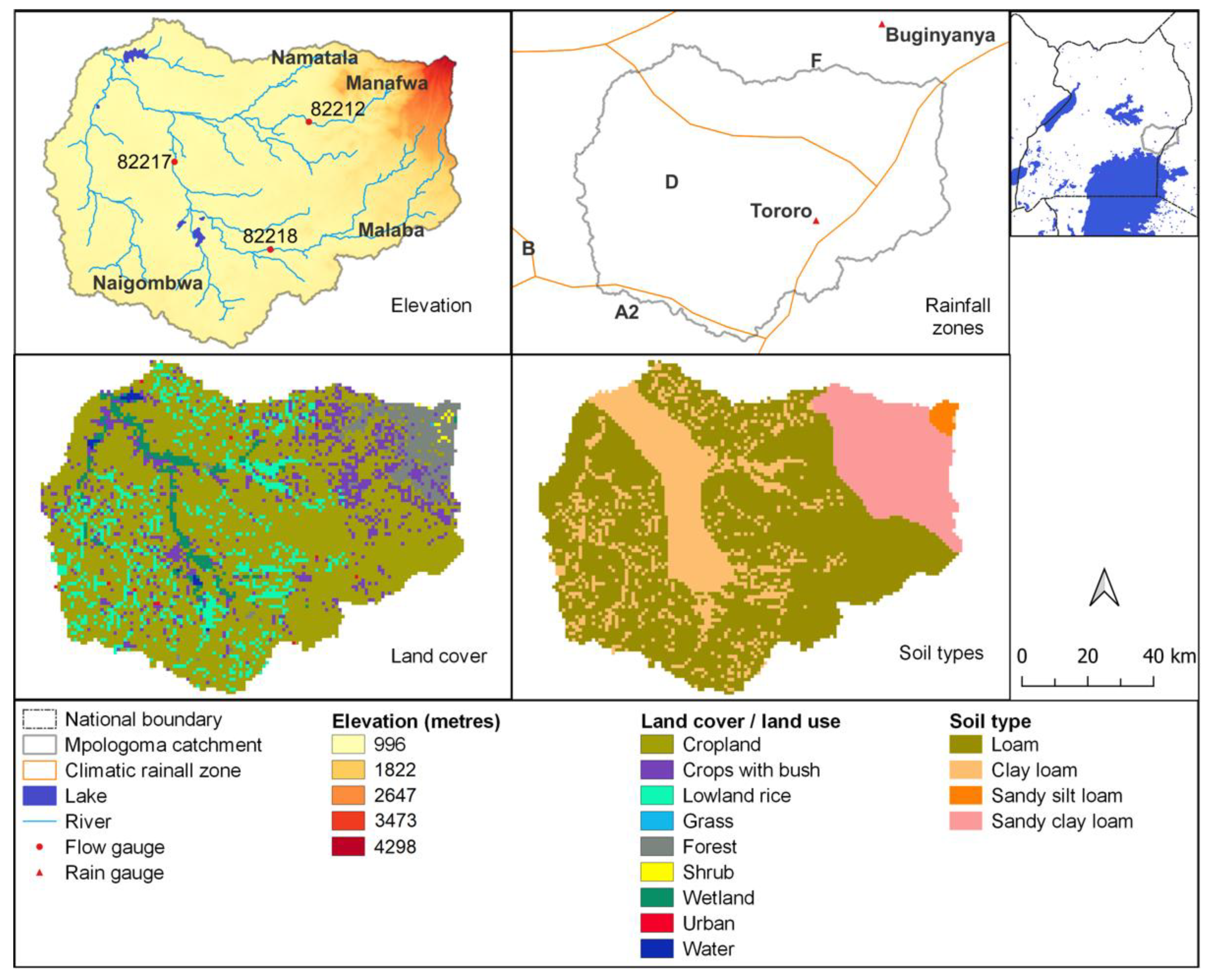
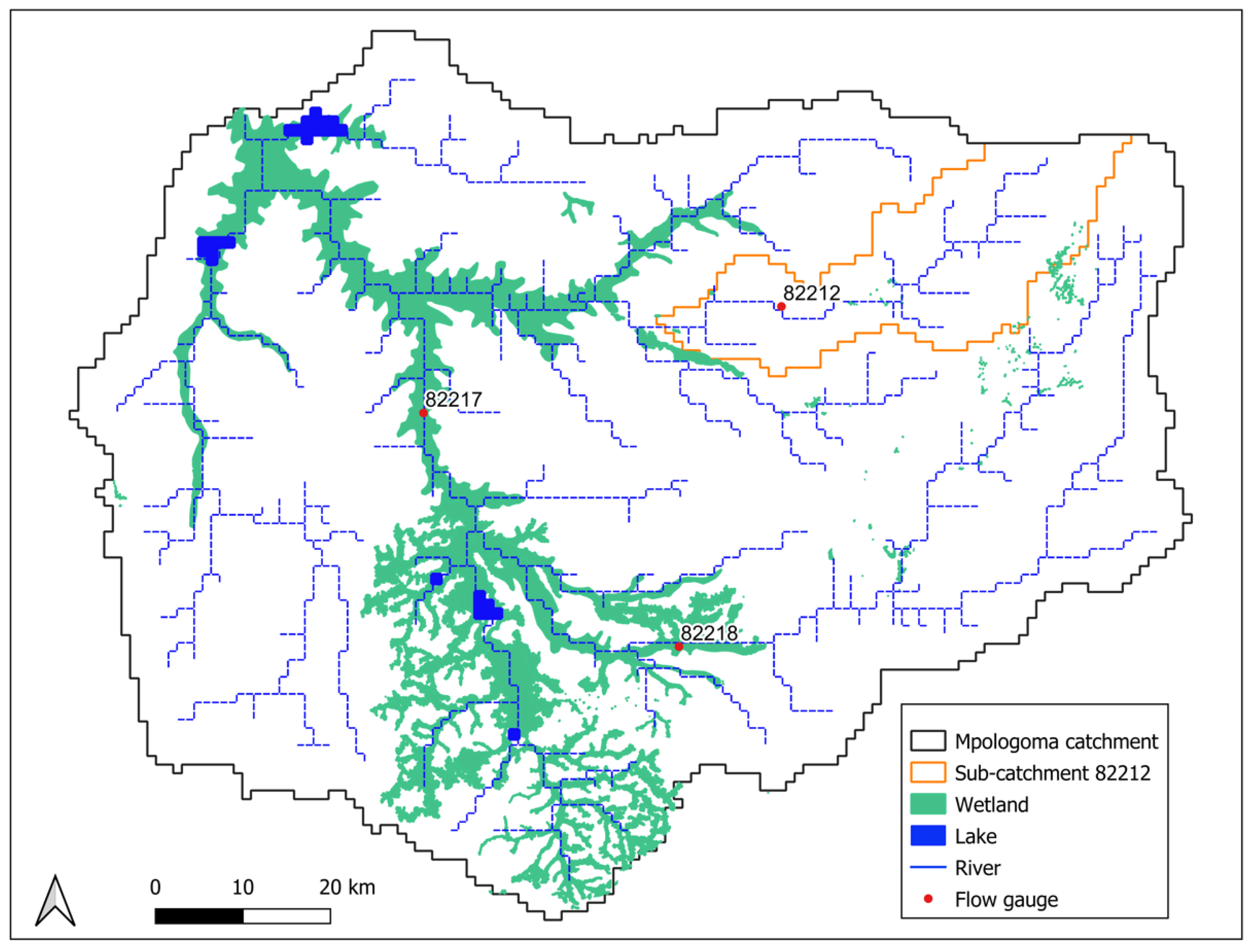
2.1. Study Area

The Mpologoma catchment, located between longitude 33.4–33.6° E and latitude 0.3–1.3° N, is a transboundary watershed between Uganda and Kenya (Figure 1) with over 80% of its area in Uganda. Covering 8989 km2 [46], its highest peak, Mount Elgon, is to the northeast and at approximately 4298 m above sea level (a.s.l). A more significant part of the catchment (over 80%) lies between 996 and 1150 m a.s.l, the former being the mean lake level at Lake Kyoga, Mpologoma’s outlet. Key tributaries include Namatala, Manafwa, Malaba, and Naigombwa. The region’s rainfall regime is bimodal (peak months of March to May and August to November) [47], with a mean annual rainfall of 1215 to 1660 mm [47,48]. Following Köppen–Geiger’s climate classification [49], the catchment can be categorised as wet Equatorial Monsoonal. Subsistence farming is the main economic activity, with major crops being rice, maize, beans, groundnuts, cassava, sugarcane, etc. Seven unique land use and cover types were identified in 2019 [50]. These include woodland (6.2%), grassland (5.2%), built-up areas (11.6%), subsistence crops (53.2%), wetland (21.5%), open water (1.9%), and commercial farms (0.5%).

2.2. Data Sources and Processing

Hydrological modelling in SHETRAN requires spatially explicit input datasets of climate (precipitation and potential evapotranspiration), land surface topography, land use, land cover, and soil and lithological distribution. Measured surface flow and/or groundwater levels are also required for model calibration and validation. The following subsections describe the selection and preparation of these datasets. Figure S1 in the Supplementary Materials shows a schematisation of the steps followed in the study.

2.2.1. Selection and Evaluation of Rainfall Products

Satellite-based and reanalysis rainfall products have often been favoured for hydrological modelling in regions with low rain gauge networks, such as Sub-Saharan Africa [51,52]. However, the rainfall fields of reanalysis products are less accurate in the tropics compared to satellite estimates [53]. As the predominant rainfall over inland East Africa is convective [54], satellite products may provide more accurate data. The essential satellite-based precipitation products (SPPs) that have been applied over Africa include TAMSAT, CHIRPS, ARC, RFE, MSWEP, PERSIANN, CMORPH, and TRMM 3B42 (Table A1 in Appendix A).
This study evaluated the SPPs mentioned above by ground truthing (i.e., direct comparison with rain gauge data) followed by hydrological modelling. Point-to-pixel ground-truthing, with gauges at the point scale and SPPs at the grid scale, was carried out for climatological rainfall zones D and F (Figure 1) at daily and monthly time scales, which was preceded by quality control of gauge data, as outlined in Maidment et al. [53]. The point-to-pixel comparison was used to eliminate interpolation error, which is a concern for regions with sparse gauge networks [55]. Given that RFE2.0 and MSWEP2.2 start and end, respectively, in January 2001 and October 2017, evaluations were limited to January 2001 and December 2016. Overall, 0.79% and 12.25% of gauge records for Tororo and Buginyanya, respectively (Figure 1), were not included in the assessment due to missing data.
Following other studies on Africa (e.g., [56,57]), the point-to-pixel evaluation comprised assessment for accuracy in daily rainfall identification and daily and monthly rainfall totals. The extent of rainfall identification was assessed through measures of False Alarm Ratio (FAR), Probability of Detection (POD), Frequency Bias (FB), and Heidke skill score (HSS) (the equations are in Section S2 of the Supplementary Materials). In contrast, rainfall totals were assessed through correlation coefficient (R) and Nash–Sutcliffe efficiency (NSE). FAR represents the fraction of satellite-estimated rain days not captured by the gauge, and POD is the fraction of gauge rainfall days identified by the satellite product. FB is the ratio of total rain days in the satellite product to that of the gauge. It ranges from 0 to ∞, with values less (greater) than one indicating under (over) estimation of rain days. HSS, on the other hand, assesses the overall skill of a satellite product’s rain-day detection while accounting for random chance. Its value ranges from −∞ to 1, with zero indicating that the satellite product cannot detect rain days. A value less than zero implies that random chance is better than the product, whereas one denotes perfect skill.
MSWEP, TAMSAT, and CHIRPS performed best at the monthly timescale (see results in Appendix B). These SPPs were then hydrological assessed to select the best SPP for the study area.

2.2.2. Estimation of Potential Evapotranspiration (PET)

Duan et al. [58] evaluated the performance of Climate Forecast System Reanalysis (CFSR) daily temperature fields over the eastern African region of Ethiopia. They concluded they are as good as the observed temperature when employed in hydrological models. Hargreaves’ method [59] uses temperature values for PET estimation, and it is recommended for regions with limited data [60]. Di Vittorio and Georgakakos [28] estimated monthly evapotranspiration rates over the Sudd wetlands in South Sudan using four different methods, including Hargreaves’. Hargreaves’ procedure performed best, with results similar to those generated using the Penman equation. Thus, this study used the CFSR daily minimum and maximum air temperature fields to calculate PET.

2.2.3. Measured Flow Data

Water level time series recorded at 08:00 and 16:00 h for 17 years (2000 to 2016) were acquired from the Ministry of Water and Environment (MWE), Uganda. The datasets comprised measurements for rivers Manafwa (Station 82212), Malaba (Station 82218), and Mpologoma (Station 82217), Figure 1. Rating curves for each station, also supplied by MWE, were used in deriving daily average flows. Given that a quality check of flow measurements is essential in hydrological modelling, the minimum steps recommended by Crochemore [61] were adopted. These include analysis of data availability (in terms of length and spatial distribution of time series) and quality checks for outliers, homogeneity, and trend. The above steps were preceded by a visual inspection of hydrographs for suspicious records (e.g., negative values, wrongly recorded missing data, and out-of-the-ordinary hydrograph patterns of variation). Data preprocessing can lower hydrologic data uncertainty by up to 10%, minimising bias and incorrect conclusions [62].

2.2.4. Land Surface Representation

Coarse grids are often adopted in physically based, spatially distributed models to lower unknowns and execution time [63], which increases prediction uncertainty [64]. However, 0.5 to 4 km grid scales are generally acceptable for flow prediction in large catchments. For example, Sreedevi and Eldho [64] simulated discharge and sediment yield at 1 and 4 km grid scales based on effective parameters of a 2 km SHETRAN model. No significant difference was detected in the monthly flow predictions. Similarly, Zhang [65] compared the SHETRAN model performance at 0.5, 1, and 2 km grid scales. Performance generally improved with grid resolution. Nonetheless, the 1 and 2 km grids gave good results. Although DEM resampling techniques do not significantly influence streamflow modelling [66], resampling to coarser grids greater than 1 km could substantially affect the spatial distribution of land use, soil types, and river links, which can affect model performance in capturing peak flows and runoff volumes [65]. Thus, for this study, the Advanced Space-borne Thermal Emission and Reflection Radiometer (ASTER) Global Digital Elevation Model (DEM) Version 3 [67], initially at 30 m × 30 m grid resolution, was resampled to 1 km × 1 km grid size and used in defining catchment boundary, ground surface elevations, and generating river flow paths.

2.2.5. Land Cover and Land Use Layer

The European Space Agency (ESA) Climate Change Initiative (CCI) land cover map [68] was used in categorising land use/cover in the study area. ESA CCI provides annual global land cover layers at 300 m spatial resolution from 1992 to recent times, with accuracies varying from 71% to 97% depending on the land use/cover type [68]. No significant change in permanent (i.e., papyrus-dominated) wetland areas was detected from 2000 to 2020. Thus, model calibration and validation used the 2007 land cover layer (Figure 1). Detailed information on ESA CCI land cover layers is online at https://www.esa-landcover-cci.org/.

2.2.6. Soil and Lithology

The FAO/UNESCO Digital Soil Map of the World version 3.6 [69] was used in defining soil categories. However, soils in some wetland areas and small water bodies were not correctly categorised. The topsoil in these areas is mostly clay loam [46]. Thus, the land cover map was used in identifying these locations, and the soil category was reclassified accordingly. As with the DEM, the soil layer was resampled to a 1 km × 1 km grid. Four soil types (loam, clay loam, sandy silt loam, and sandy clay loam) were identified in the catchment (Figure 1).
Lithological depths were estimated from borehole log data for the study area (1986 in total). Analysis of the records indicates 1668, 195, and 123 logs in the regions dominated by loam, clay loam, and sandy clay loam, respectively. No log data were available for the area dominated by sandy silt loam. Thus, its lithological depths were assumed to be the same as the soil category closest to it, sandy clay loam. In addition, sandy silt loam covers less than 1% of the catchment. Overall, three critical lithological layers (topsoil, weathered rock, and base rock) were identified from the log data (Table 1).

2.3. Modelling Approach

SHETRAN [39] is a 3D integrated surface and subsurface finite difference modelling system for water flow, sediment transport, and contaminant transport in catchments. Its water flow components comprise interception and evapotranspiration, overland and channel flow, variably saturated lithology and aquifers, and channel–aquifer interactions. The model’s xy grid was set at 1 km × 1 km, with 35 cells in each grid column. The lithological cells ranged from 0.1 to 0.2 m in the topsoils but were set to 5 m in the rock layers. Selection of the number of cells is a trade-off between accuracy and simulation time. Generally, the cells are smaller nearer the surface (as the flow is more variable) and larger as you go down the column. Although models were driven with daily data (precipitation and evapotranspiration), the simulation timestep was set to 1 h. Detailed information on SHETRAN can be accessed at https://research.ncl.ac.uk/shetran/.
Model calibration and validation, preceded by sensitivity analysis (see Appendix C). In Phase 1, the second step for precipitation product evaluation (i.e., hydrological evaluation of SPPs), SHETRAN was calibrated and validated on the sub-catchment gauged at station 82212 (Figure 2). The calibration and validation were carried out independently for each SPP (i.e., MSWEP, TAMSAT, and CHIRPS) that performed relatively well in the ground-truth evaluation. The sub-catchment gauged at 82212 has an insignificant wetland coverage. Thus, it enabled model parameterisation for catchments without wetlands in the region.
In Phase 2, the entire Mpologoma catchment was simulated, with parameters initially set to the effective values attained in Phase 1. The Phase 2 model was set up only for the precipitation product that performed best in Phase 1. Recalibration and revalidation on stations 82217 and 82218, respectively, were carried out with parameter adjustments limited to locations with wetlands.
River channels in the SHETRAN model flow along the edge of grid squares and are automatically created from the DEM. However, due to weaknesses in the SHETRAN automatic river generator in the flatter wetland areas, they were manually adjusted to follow the actual river network. River channels were removed where there are lakes, and the elevations of grid squares in lake locations were changed to depict average lake depths. The modified files were used in SHETRAN (version 4.4.5). Model performances were assessed statistically by quantifying the Nash–Sutcliffe efficiency (NSE), percent bias (Pbias), and the root mean square error standard deviation ratio (RSR). These metrics are generally recommended for model performance assessment in hydrology [70].

2.4. Impacts of Wetlands on Catchment Discharge

Wetland flow regulating functions can be assessed if a reference condition is defined, against which flow changes associated with the wetland are quantified [71]. Bullock and Acreman [72] documented the most used approaches for inferring wetland flow regulating functions. The ‘with/without’ approach, restricted to model-based studies, compares the same catchment with and without wetlands. The model is typically calibrated and validated for a ‘with’ or ‘without’ scenario. Simulations are then carried out with the alternate scenario, and any difference between the model outputs is attributed to the existence of wetlands. Papyrus plants are perennial herbaceous vegetation. Although communities around them harvest papyri in the dry season, they quickly regenerate at the onset of rains [12]. This study assumed that papyri stand remains the same all year round.
Furthermore, hydrological measures (flow indices) are employed in quantifying wetland flow regulating functions. These measures can be broadly classified into five groupings [72]: gross water balance, groundwater recharge, baseflow and low flows, flood response, and river flow variability. In this study, the historical impacts of wetlands on catchment flow were assessed using indices of baseflow and quickflow. In contrast, future effects were evaluated using flood and low flow indices. Quickflow is the part of precipitation that reaches the river fastest through surface runoff and interflow and is mainly responsible for floods. Thus, baseflow and quickflow are good indicators of how wetlands respond to slow and fast flow processes. However, a more holistic approach to catchment management requires the characterisation of flows in terms of flood/low flow indices (e.g., magnitude, duration, frequency, etc.) [73]; thus, it was adopted for the future period.

2.4.1. Impacts of Wetlands on Baseflow and Quickflow

The Wetland Specific Impact (WSI) metric [74] was employed in quantifying wetland flow regulating functions. It normalises the hydrological impact, which is an increase or decrease in flow metrics with respect to the wetland area (Equation (1)).
WSIBF/QF = [RBFw/QFw − RBFwo/QFwo] ÷ A
where WSI (m3/s/km2) is the index of wetland impact expressed as a flow parameter (baseflow (BF) or quickflow (QF)) per unit area of wetland; R (m3/s) is discharge (baseflow or quickflow) for the situation with (w) and without (wo) wetlands; and A (km2) is the total wetland area.
The hydrological impacts of wetlands are highly dependent on climatic conditions, leading to seasonal and inter-annual variability [74]; thus, WSI values were computed at monthly and annual timescales. Boxplots showing the mean, median, and interquartile range and upper and lower limits were employed to illustrate this variability. However, only the mean WSI values and non-outlying WSI range (upper and lower limits) were used to describe wetlands’ roles. WSI values were computed over 30 years (1984 to 2013) for the model outputs forced with ‘observed’ climatic data (i.e., MSWEP and CFSR, Table 2). Baseflow and quickflow components were extracted from total flows using WETSPRO, a flow filtering tool based on the extended Chapman filter [75] and available online at https://bwk.kuleuven.be/hydr/pwtools.htm#Wetspro (accessed on 10 August 2022).

2.4.2. Impacts of Wetlands on Future Flood and Low Flows

This study assessed climate change impacts using the first ensemble (r1i1p1f1) daily climate variables from the Coupled Model Intercomparison Project phase 6 (CMIP6). Given that suitable corrections can only be attained if the scale gap between the model and observational data is realistic [76], the CMIP6 models were restricted to 100 km nominal resolution. Thus, only four (GFDL-ESM4, CESM2-WACCM, MRI-ESM2-0, and NorESM2-MM) of the nine CMIP6 models (Table A2 in Appendix A) recommended for application over the East African region were selected. As of July 2022, CESM2-WACCM had no historical minimum and maximum temperature at the official CMIP6 web portal (https://esgf-node.llnl.gov/projects/cmip6/). Thus, GFDL-ESM4, MRI-ESM2-0 and NorESM2-MM were the only Global Climate Models (GCMs) used. These GCMs were bias-corrected using the quantile delta mapping method in RStudio’s ‘MBC’ package [77], with daily MSWEP and CFSR as observed precipitation and temperature fields, respectively.
The focus was on the impacts of representative concentration pathway 8.5 (RCP8.5), given that current greenhouse gas emissions are closer to it than the other RCPs [78]. Although there is consensus to limit warming to 2 °C [79], Intergovernmental Panel on Climate Change (IPCC) predictions indicate end-of-century warming of up to 4 °C if the current emission trend continues [80]. Thus, this study assessed climate change impacts at 2 and 4 °C global warming levels (GWLs), with NOAA GISS Surface Temperature Analysis [81] global observational data as a reference. A collection of 30-year windows corresponding to 2 and 4 °C GWLs were extracted for each GCM, following the method in Vautard et al. [82].
Following Xu et al. [83], the mitigating effects of wetlands on future flood flows were assessed using flow duration, magnitude, and frequency indices by analysing model outputs with and without wetlands. These were similarly adapted for low flows. Table 2 shows the total number of simulations carried out with the various CMIP6 datasets at the baseline (BL), GWL2 and GWL4. A 2-year return period flood and low flow threshold of the baseline scenario were used to detect the occurrence of flood and low flows, assuming that river cross sections do not change at GWL2 and GWL4. The 2-year threshold is often used as an estimate of bank-full discharge [84], thus a proxy for flood flow (i.e., starting point of inundation). The same return period was chosen for low flow as a review of droughts over Africa showed that, in the worst case, droughts occur every two years in Uganda [85]. A flood event was considered one or more consecutive days when the daily flow was larger than the bank-full flow. Similarly, a low flow event is one or more consecutive days when daily flow is less than or equal to the low flow threshold. The estimated 2-year return period flood and low flow threshold of the baseline scenario are 33.2 and 11.5 m3/s, respectively.
The various flow indices were calculated over the water year (March to February). Flow duration was calculated as the average of individual events in a water year. The average per event was calculated before averaging over a year for flow magnitude. Flow frequency is the number of flood or low flow events yearly. The analysis assumed the same wetland size for baseline and future scenarios.
Table 2. List of models (with and without wetlands) simulated/forced with ‘observed’ (i.e., MSWEP and CFSR) and CMIP6 climatic datasets.
S. No.Climatic DatasetsSimulation Period (Model Warmup)Wetlands Present or Not
1MSWEP rainfall and CFSR PET1979–2013 (1979–1983)Yes
2No
3GFDL-ESM4 at BL1979–2013 (1979–1983)Yes
4No
5MRI-ESM2-0 at BL1979–2013 (1979–1983)Yes
6No
7NorESM2-MM at BL1979–2013 (1979–1983)Yes
8No
9GFDL-ESM4 at GWL22028–2063 (2028–2032)Yes
10No
11MRI-ESM2-0 at GWL22030–2065 (2030–2034)Yes
12No
13NorESM2-MM at GWL22025–2060 (2025–2029)Yes
14No
15GFDL-ESM4 at GWL42059–2094 (2059–2063)Yes
16No
17MRI-ESM2-0 at GWL42051–2086 (2051–2055)Yes
18No
19NorESM2-MM at GWL42049–2084 (2049–2053)Yes
20No

3. Results

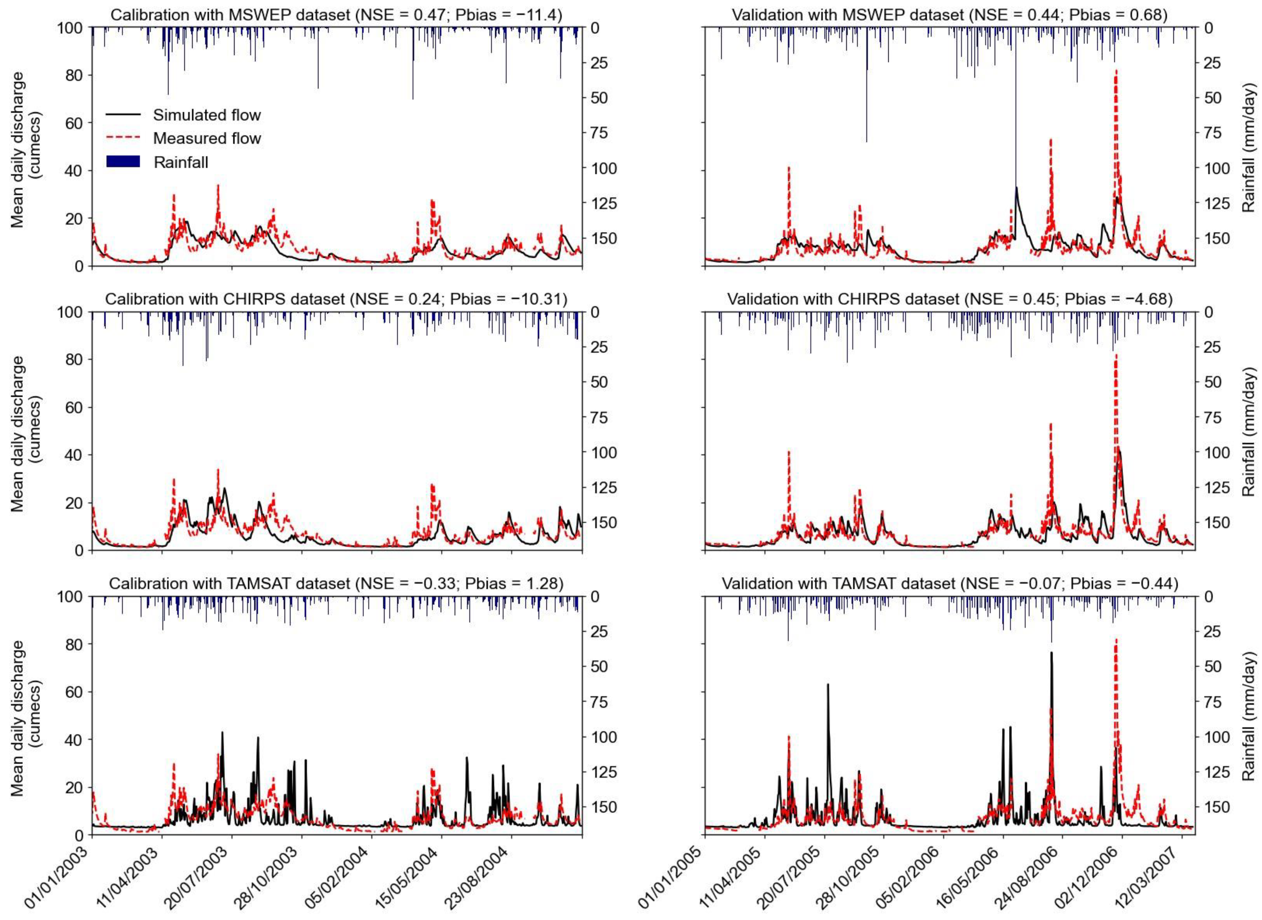
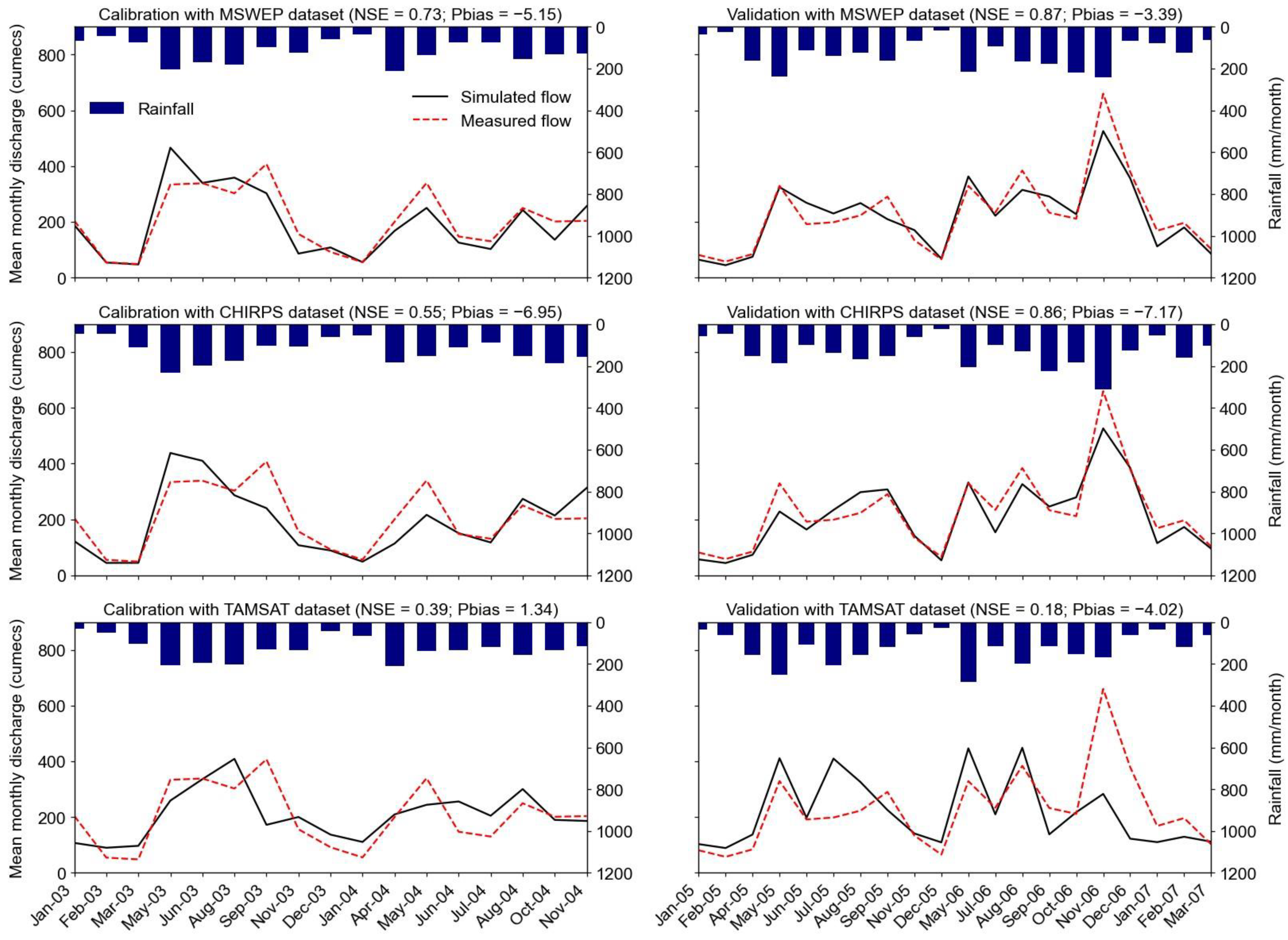
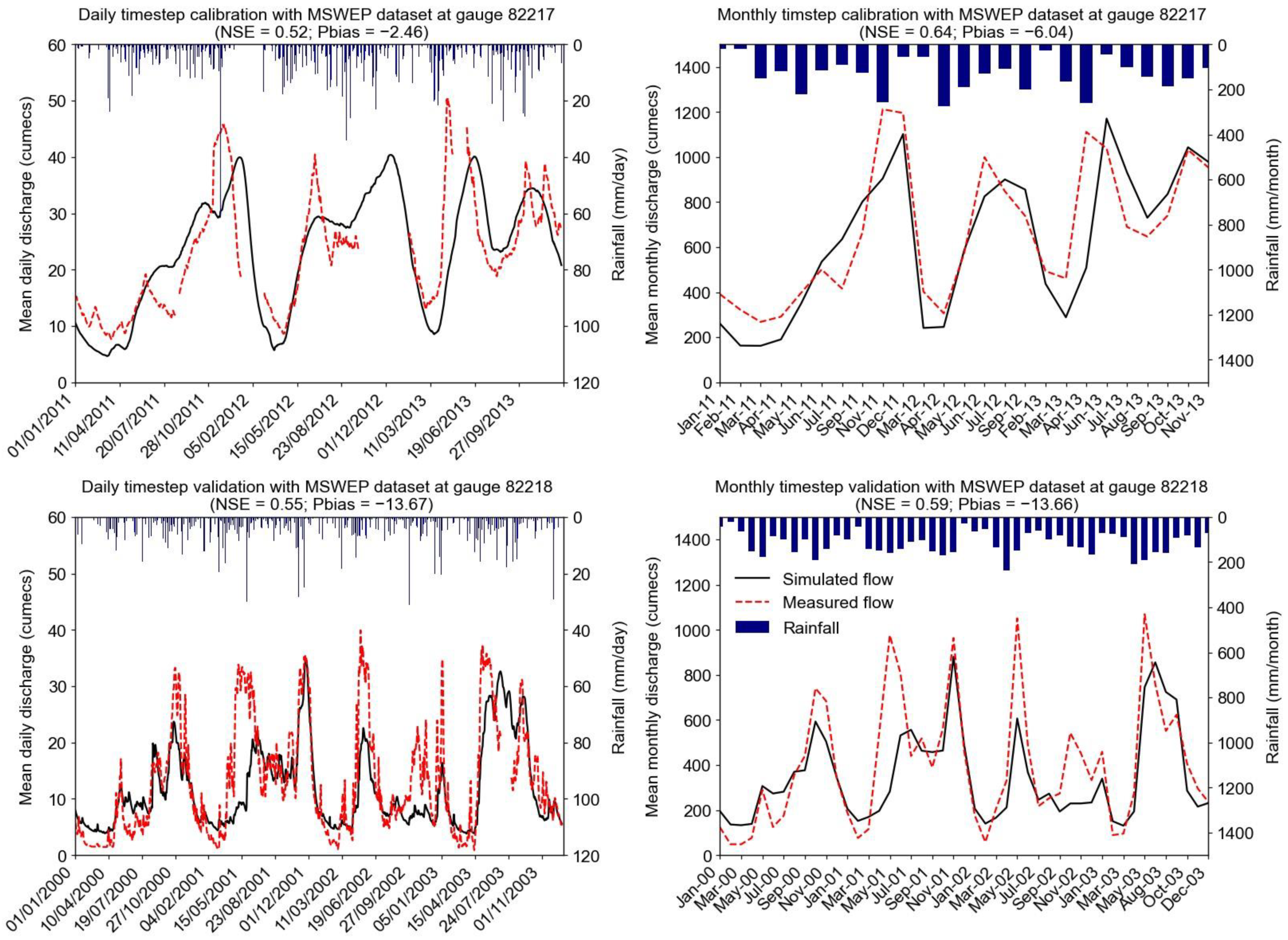
3.1. Model Calibration and Validation Results

Phase 1 model calibration and validation results for the best performing SPPs (MSWEP, TAMSAT, and CHIRPS) are shown in Figure 3 and Figure 4 for daily and monthly timesteps, respectively. Overall, MSWEP performed best with a daily NSE (Pbias/RSR) and monthly NSE (Pbias/RSR) of 0.47 (−11.4%/0.73) and 0.73 (−5.15%/0.52) at calibration and 0.44 (−0.68%/0.75) and 0.87 (−3.39%/0.36) at validation. CHIRPS followed this at 0.24 (10.31%/0.87) and 0.55 (−6.95%/0.67) for calibration and 0.45 (−4.68%/0.74) and 0.86 (−7.17%/0.38) for validation. Meanwhile, TAMSAT attained −0.33 (1.28%/1.16) and 0.39 (1.34%/0.78) at calibration and −0.07 (−0.44%/1.03) and 0.18 (−4.02%/0.9) at validation. Model performance generally improves with timestep and concurs with studies over Africa (e.g., [43,86]) that recommend hydrological performance assessment of SPPs at longer timescales (e.g., monthly instead of daily). This is because validation errors in SPPs are often offset upon spatial and temporal integration at the catchment scale [87]. In addition, real-time control, design, and management of most catchment systems (such as irrigation and water supply, reservoirs, land use change, climate change, and environmental impact studies) can be achieved with monthly hydrological model estimates [88]. Mutenyo et al. [89] modelled the catchment gauged at 82212 using SWAT, a semi-distributed hydrological model, with daily gauge rainfall data from 1955 to 1961. The model performed best at the monthly timescale with NSE values (Pbias) of 0.72 (−0.49%) and 0.64 (20.5%) for calibration and validation, respectively, which are similar to the results obtained in this study.
Given its superiority in this study, MSWEP was further used in Phase 2 of model calibration and validation, focusing on the recalibration of channel Strickler coefficient (Krc) in locations with wetlands. Strickler coefficient is the inverse of Mannings coefficient. An optimal Krc of 7 m1/3/s, from an initial value of 30 m1/3/s (Phase 1), denoting a 76.6% change in Strickler coefficient, was attained, with daily and monthly NSE (Pbias/RSR) of 0.52 (−2.46%/0.69) and 0.64 (−6.04%/0.6) at calibration and 0.55 (−13.67%/0.69) and 0.59 (−13.66%/0.64) at validation, respectively (Figure 5). To ensure the robustness of the Phase 2 model, calibration and validation were carried out at two different sites (82217 for calibration and 82218 for validation). Due to uneven data gaps in the records of the two gauging stations, calibration was carried out from January 2011 to November 2013, whereas validation was from January 2000 to December 2003.

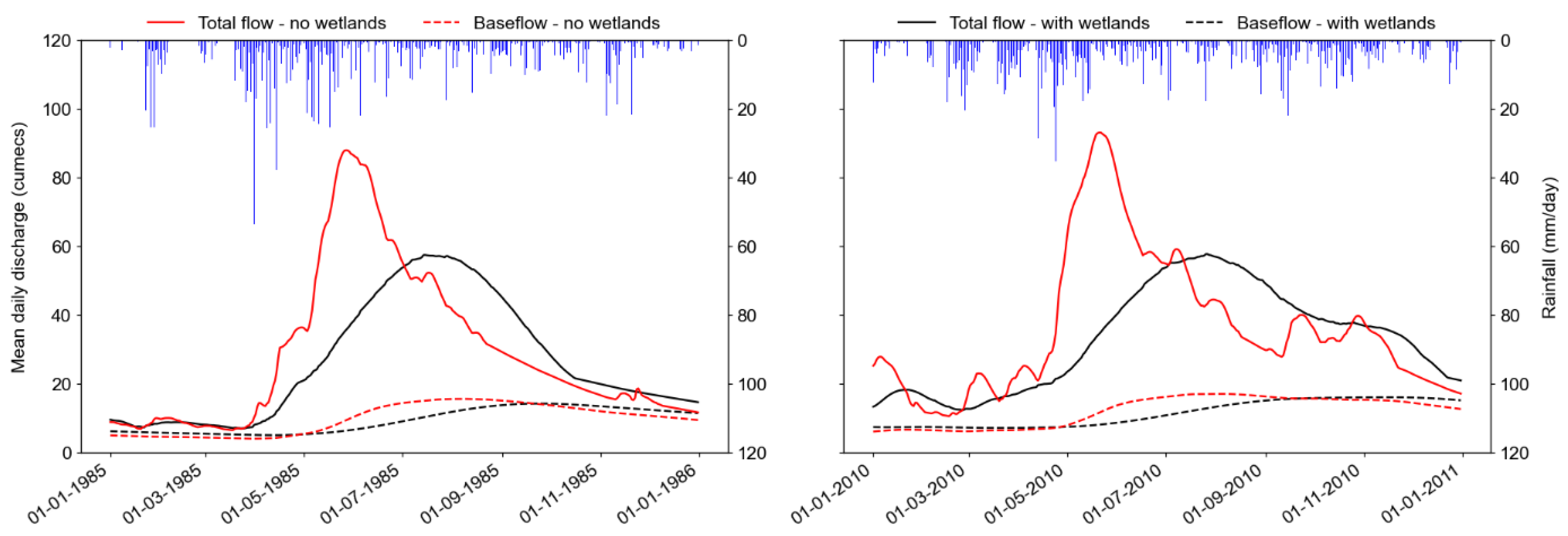
3.2. Historical Impacts of Wetlands on Catchment Hydrology

3.2.1. Overall Impacts of Wetlands on Catchment Hydrology

The mean annual water balance components over the Mpologoma catchment are shown in Table 3. Precipitation (P), actual evapotranspiration (AET), and catchment outflow (Q) were extracted from the SHETRAN model output for the situation with and without wetlands over the period 1984 to 2013 (30 years). The models were driven with MSWEP and CFSR precipitation and PET datasets. Overall, wetlands modulate river flow in the Mpologoma catchment by decreasing annual discharge by 5.5% on average. In contrast, evapotranspiration is enhanced annually by 0.4% on average.

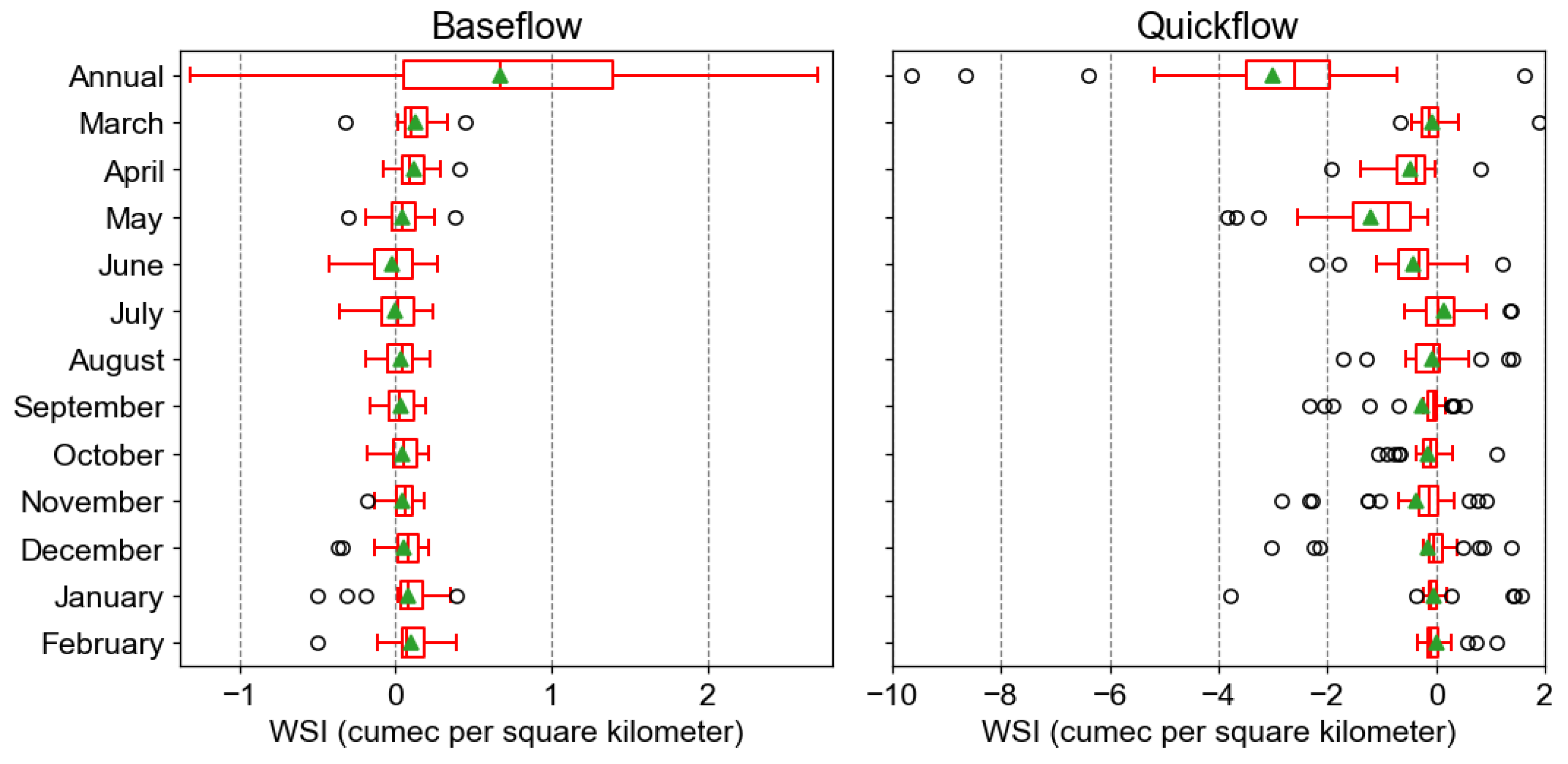
3.2.2. Impacts of Wetlands on Baseflow and Quickflow

Based on mean WSI values (Figure 6), wetlands moderately support baseflow at the catchment scale in most months of the year except June (WSI of −0.02 m3/s/km2). Quickflow is suppressed in most months, except July and February (positive WSI of 0.16 and 0.01 m3/s/km2, respectively). Negative baseflow and positive quickflow WSI values indicate a reversal of the supportive role of wetlands towards these flow components, whereas zero implies a null response. The critical periods during which baseflow is often positively impacted are from March to May (WSI of 0.13, 0.12 and 0.05 m3/s/km2, respectively) and from October to February (WSI of 0.05, 0.05, 0.05, 0.08 and 0.1 m3/s/km2, respectively). Meanwhile, the corresponding periods for quickflow are from April to June (WSI of −0.48, −1.21 and −0.43 m3/s/km2, respectively) and September to November (WSI of −0.25, −0.16 and −0.36 m3/s/km2, respectively).
At the annual timescale, wetlands generally enhance baseflow (mean WSI = 0.68 m3/s/km2) and attenuate quickflow (mean WSI = −3 m3/s/km2). However, the yearly WSI non-outlying range shows that wetlands significantly reduced quickflow (−5.19 to −0.71 m3/s/km2) compared to enhanced baseflow (−1.31 to 2.7 m3/s/km2).

3.3. Impacts of Wetlands on Future Catchment Hydrology

3.3.1. The Overall Impact of Wetlands on Future Catchment Hydrology

The mean annual water balance components over the Mpologoma catchment for the ensemble baseline (BL), GWL2 and GWL4 are summarised in Table 4. Like the water balance for the models driven by MSWEP and CFSR precipitation and PET products (Table 3), water balance components were extracted over 30 years, with the baseline period set from 1984 to 2013. GWL2 and GWL4 water balance components are tied to a future 30-year period with a mid-point at 2 and 4 °C global warming levels, respectively. As the various individual GCM products were bias-corrected with MSWEP and CFSR datasets, model predictions for the BL are similar to those driven by MSWEP and CFSR. Wetlands in the BL modulate river flow by decreasing annual discharge (−6.6%) while enhancing evapotranspiration (0.4%) on average. These effects continue with warming but with a reduced impact on discharge.

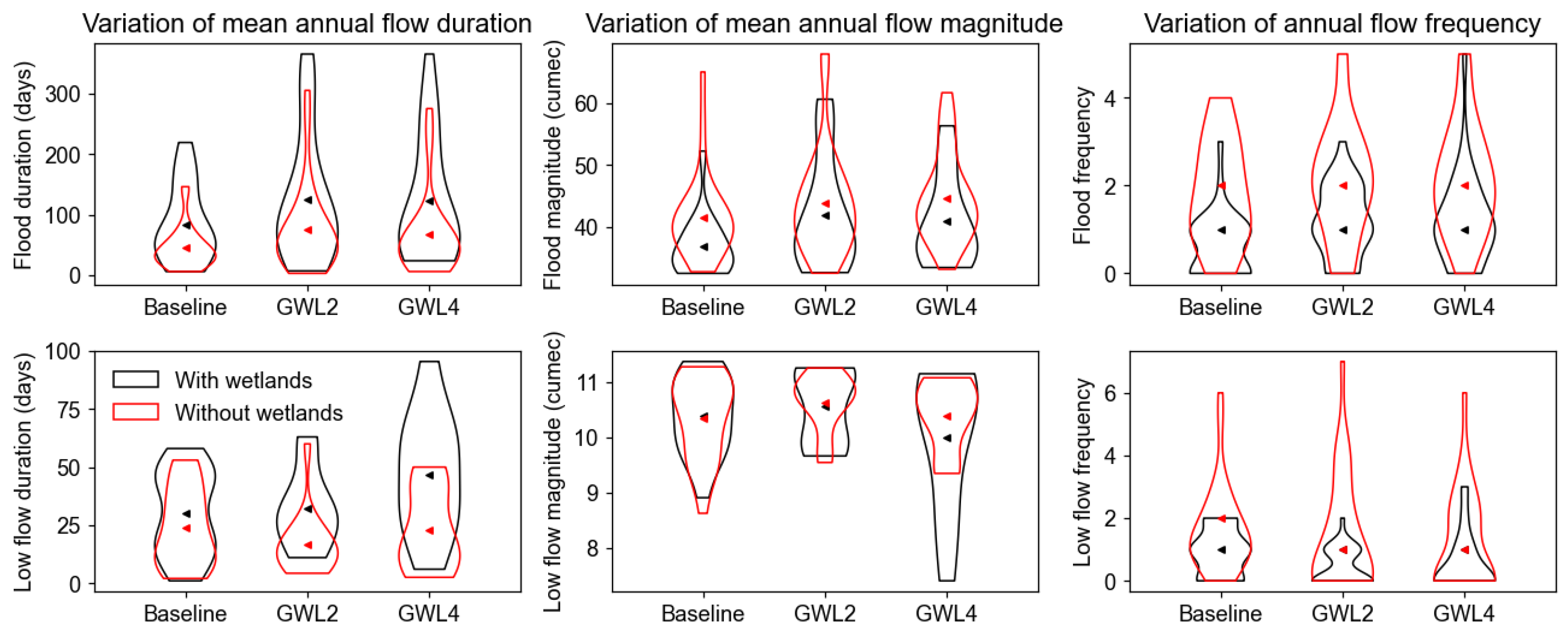
3.3.2. Impacts of Wetlands on Future Flood and Low Flows

Figure 7 shows violin plots of flood and low flow indices for the situation with and without wetlands. For flood flows and a particular catchment treatment (i.e., with or without wetlands), the 30-year mean value (Table 5) indicates that both duration and magnitude increase with warming. However, the difference between GWL2 and GWL4 indices is minimal. For the situation with wetlands, the mean flood duration per event increases from 85 days at BL to 128 and 110 days at GWL2 and GWL4, respectively. Similarly, for the situation without wetlands, the duration increases from 46 days at BL to 72 and 61 days at GWL2 and GWL4, respectively. The mean flood magnitude per event, for the situation with wetlands, increases from 37.65 m3/s at BL to 42.87 and 41.21 m3/s at GWL2 and GWL4, respectively. For the case without wetlands, the magnitude per event increases from 42.23 m3/s at BL to 45.21 and 44.7 m3/s at GWL2 and GWL4, respectively. In general, wetlands in the Mpologoma catchment are predicted to increase the mean flood duration by 77.8% (56 days) and 80.3% (49 days) at GWL2 and GWL4, respectively, and lower the mean flood magnitude by 5.2 and 7.8%.
From Table 5, the estimated mean flood frequency is constant, irrespective of warming level, at 1 and 2 flood events per year for the situation with and without wetlands, respectively. However, the potential for a larger number of flood events in a year (the range) increases with warming. For example, for the situation with wetlands, annual flood events increase from the BL range of 0–2 flood events to 0–3 and 0–4 events at GWL2 and GWL4, respectively. For the situation without wetlands, the range increases from 0–4 to 0–5 at both GWL2 and GWL4.
Unlike flood flows, the impacts of warming levels on low flows are generally heterogeneous. For example, for the situation with wetlands, the mean low flow duration at GWL2 (33 days) is the same as that at BL (32 days) but increases to 48 days at GWL4. However, the range of low flow duration per event increases with warming from 3–59 days at BL to 14–65 and 15–97 days at GWL2 and GWL4, respectively. Similarly, for the situation without wetlands, the mean low flow duration at GWL2 (19 days) is the same as that at BL (22 days) but increases to 27 days at GWL4. The range, however, increases with warming from 2–53 days at BL to 5–61 and 3–88 days at GWL2 and GWL4, respectively. In general, wetlands are projected to increase future mean low flow duration by 73.7% (14 days) and 77.8% (21 days) at GWL2 and GWL4, respectively.
For the case of low flow magnitude, there is no significant change in the 30-year mean flow value, irrespective of catchment treatment. For example, for the situation with wetlands, the mean flow magnitude per event increases and drops minimally from 10.42 m3/s at BL to 10.6 and 10.04 m3/s at GWL2 and GWL4, respectively. Similarly, for the situation without wetlands, it increases and drops minimally from 10.47 to 10.71 and 10.45 m3/s, respectively. No significant change can be seen in the range of low flow values, except for GWL4 with wetlands. The range of low flow magnitude increases from 8.91–11.4 m3/s at BL to 7.4–11.17 m3/s at GWL4. In general, though not significant, projections suggest that wetlands will reduce future mean low flow magnitude by 1 and 3.9% at GWL2 and GWL4, respectively. However, a considerable decline of 21.2% is expected in the lower limit of low flow at GWL4.
The mean low flow frequency is generally constant, irrespective of the warming level. On average, one low flow event occurs per year regardless of catchment treatment. However, the range of low flow events is lower for the situation with wetlands. Events vary from 0–2 and 0–4 at GWL2 and GWL4, respectively, compared to 0–7 and 0–6 for the situation without wetlands. Overall, though wetlands are predicted to negatively impact future low flow magnitude and duration, they are expected to positively impact low flow frequencies by lowering the range of events in a year by 71.4 and 33.3% at GWL2 and GWL4, respectively.

4. Discussion

4.1. Historical Impacts of Wetlands on Catchment Hydrology

The catchment water balance (Table 3) shows that the Mpologoma floodplain wetlands reduce annual average river flow, increase evapotranspiration compared to most land types, and enhance groundwater recharge. The response is typical of wetlands, depending on the underlying lithology [72]. Additionally, the mean annual WSI, depicting enhanced baseflow and attenuated quickflow, show that wetlands regulate flow variability at the catchment scale [90]. Past studies in Africa, although restricted to wetland complexes (e.g., the Sudd wetland in South Sudan [22,23] and the Okavango Delta in Botswana [23]), have also shown that papyrus-based riparian wetlands play significant roles in dampening flow variability. The greater impact on quickflow compared to baseflow, as seen in this study’s WSI non-outlying range, concurs with the work by Kadykalo and Findlay [91], who concluded that wetlands perform better in flood mitigation than low flow augmentation. Overall, the mean annual WSI values show that wetlands in the Mpologoma catchment are at least four times better at attenuating quickflow than enhancing baseflow. Like the mean annual WSI values, the mean monthly WSI results show that papyrus wetlands are most effective in curtailing quickflow. The periods in which quickflow is suppressed coincide with the region’s wet seasons (March to May and September to November).
Although the mean monthly WSI shows baseflow enhancement in most months, reversal of the supportive role of wetlands occurs in the first dry season (June to July). One would expect baseflow enhancement and nearly zero quickflow WSI during the first dry season (June to July), as seen in the second dry season (December to February). The disparity between the two dry periods could be due to the different antecedent conditions. Both dry periods start immediately after a wet period; however, the first rainy season is much wetter than the second, and the second dry spell is much drier [47]. This affects storage and connectivity pathways between wetlands and rivers. Hydraulic gradients and hydrological connectivity in riparian wetlands, typical of those in the Mpologoma catchment, depend on adequate water levels in both the river and wetlands, thus influencing discharge to or recharge from rivers [74]. This exchange of fluxes between wetlands and rivers is driven by catchment scale factors such as rainfall (intensity and duration), landscape (topography, soil and geology, drainage area, land use, and land cover), and initial conditions [91,92,93]. Kayendeke and French [24] showed that, for a microsite of 0.18 km2 in the Naigombwa sub-catchment of the Mpologoma catchment, papyrus wetland flows are dominated by surface inflows, with negligible contribution from groundwater (i.e., wetland soils are mostly heavy clay loam). The lack of baseflow support from wetlands in June–July may result from a reversal in hydrological dynamics between rivers and wetlands, as shown in Figure 8. The figure shows hydrographs of baseflow and total flow for water years 1985 and 2010 when wetlands reduced baseflow by the largest amount in June and July. For these two years, baseflow with wetlands was, respectively, 0.61 and 0.64 of the baseflow with no wetlands for June and 0.69 and 0.72 for July. Figure 8 indicates that the wetland’s supportive role of providing baseflow discharge to rivers was reversed between May and September. This reversal was also observed by Kayendeke and French [24] for the site mentioned above between July 2015 and January 2016. Overall, wetland interconnections are complex at the catchment scale due to the aggregation effects of multiple wetlands on flow regimes and the influences of various flow paths [30].

4.2. Impacts of Wetlands on Future Catchment Hydrology

The projected catchment water balance (Table 4) shows that wetlands will decrease discharge at GWL2 and GWL4 but at rates lower than BL. CMIP6 models project increased precipitation over East Africa [94,95], as seen in the 30-year ensemble mean of the GCMs used in this study (Table 4 and Figure S7 in the Supplementary Materials). Thus, it explains the expected reduced effect of wetlands on the future annual discharge and the predicted increase, irrespective of catchment treatment (i.e., with or without wetlands), in the 30-year mean flood duration and magnitude and the range of flood frequencies in a year (Table 5).
Although the mean flood magnitude and the range of flood frequencies increase at GWL2 and GWL4, they are lower for the situation with wetlands. Meanwhile, the predicted mean flood duration is more significant in the case of wetlands. This agrees with other studies that show that floodplain wetlands lower flood magnitude, reduce the frequency of flooding, increase time to peak (flood duration), and delay floods [72,91].
Future predictions show that wetlands will worsen low flow’s mean duration and magnitude. Warmer climates accelerate wetland water loss through evapotranspiration [31], leading to a decline in dry season flows, particularly during severe drought [74]. Floodplain wetlands in other parts of Africa, such as Sierra Leone and South Africa, have been shown to negatively impact dry season river flow due to high evapotranspiration rates [72]. Meanwhile, wetlands in the Mpologoma catchment will positively impact future low flow frequencies by lowering the range of frequencies in a year. The predicted reduction could be associated with water storage and slow water release wetland services. Acting like a ‘sponge’, wetlands store water during the wet season and release it in the dry period [96], thus minimising low flow episodes.

4.3. Implications and Limitations

Our findings show that wetlands greatly influence the hydrological footprint (i.e., the influence of watershed features on downstream discharge) of the Mpologoma catchment. However, increased wetland conversion for crop production, the most significant driver of wetland loss in rural catchments in Uganda [97], poses threats to sustainable catchment management. Changing climates characterised by increased precipitation, typical of the East African region [94,95], coupled with large-scale wetland loss, are predicted to aggravate flood risk [98]. Bunyangha [50] estimated a wetland loss rate of 0.6% per annum between 1986 and 2019 in the Mpologoma catchment, with a predicted loss rate of 0.2% between 2019 and 2039. This calls for restoration and conservation measures, given that most urban centres and rural communities in the Mpologoma catchment rely on natural systems (upstream wetlands) for flood management. The importance of wetland restoration for flow regulation services has been exemplified in several studies such as Acreman et al. [99], Mitsch and Day [100], Wu et al. [101], and Yang et al. [102]. Furthermore, Gulbin et al. [98] demonstrated that, even if a significant change to flow regulation is not achieved upon wetland restoration under the current climate, it could provide a future complementary measure for mitigating the negative impacts of existing flood management strategies. For example, current adequate flood protection structures such as dikes could fail due to increased precipitation. Thus, restored wetlands can play important supplementary roles.
Looking at the broader impact of climate change, irrespective of catchment treatment (i.e., with or without wetlands), our projections indicate increased flood and low flow risks, a trend similar to global projections [103]. The broader impact of flood risk in the Mpologoma catchment is projected to manifest through increased mean flood magnitude and duration and increased variability in flood frequency. Low flow risks are expected to manifest primarily in the form of increased variability in duration and number of events in a year. Although mean low flow magnitude may not significantly change with warming, extreme warming (i.e., at GWL4) is predicted to significantly reduce low flows and increase their variability. These findings on the broader impact of climate change are similar to other studies in Uganda, with indications of increased future flood magnitude [104,105,106,107,108] and occurrence of drought flows [104]. Thus, there is a need for the development of sustainable catchment flood and low flow management plans.
This paper provides useful information for wetland managers and policymakers on the supportive roles played by papyrus-based wetland systems, indicating a need for their restoration and conservation. However, our results should be treated with caution, given that modelling studies on flow regulation services of wetlands tend to predict larger impacts compared to empirical studies [91]. Future climate data generally contribute the largest uncertainty to hydrologic studies [109]. Lee et al. [110] assessed the impacts of uncertainties arising from climate change data on the streamflow of a catchment with wetlands. They concluded that the variability of GCM projections was the most significant contributor to flow prediction uncertainty. Nine CMIP6 GCMs were initially identified for this study, but only three were used due to limitations on resolution. We recommend using a larger GCM or regional climate model ensemble to lower prediction uncertainty.

5. Conclusions

This study investigated the effects of papyrus-dominated wetlands on baseflow and quickflow, including future flood and low flows within the Mpologoma catchment in Uganda. With the aid of the physically based, spatially distributed catchment modelling tool SHETRAN, the study quantified the catchment-scale flow regulating roles of papyrus wetlands. Findings show that papyrus wetlands wield a strong influence on catchment hydrology. They significantly affect quickflow (including floods), with a minor role on baseflow and most low flow indices. This indicates that wetland management is integral to water resources and flood management, particularly in tropical Africa, where papyrus wetlands naturally occur. These wetlands provide nature-based solutions against floods to several communities in the developing nations of Africa, thus providing solutions to challenges faced by flood engineers and water resources managers.
The modelled high wetland evapotranspiration rates with increased risks of low flows, especially in dry years, indicate an exaggeration of water scarcity. However, conservation decisions on whether papyrus wetlands are essential despite water scarcity risks should be taken in the broader context, depending on other wetland functions (e.g., biodiversity, human health and food, flood mitigation, recreation, etc.).

Supplementary Materials

The following supporting information can be downloaded at: https://www.mdpi.com/article/10.3390/land12122158/s1, Figure S1: Schematisation of steps followed in the study; Table S1: FAR, POD, FB and HSS at Tororo and Buginyanya rain gauge stations over January 2001 and December 2016; Figure S2: Scatter plots of daily rainfall total of SPPs and rain gauge data at Tororo and Buginyanya. The dashed line shows the perfect fit that could be attained if the gauge and SPP data were equal; Figure S3: Bar graphs of percent bias, mean absolute error and Nash-Sutcliffe efficiency at daily timescale for the various SPPs at Tororo and Buginyanya; Figure S4: Scatter plots of monthly rainfall totals (satellite products against gauge) at Tororo and Buginyanya. The dashed line shows the perfect fit that could be attained if the gauge and SPP data were equal; Figure S5: Bar graphs of percent bias, mean absolute error and Nash-Sutcliffe efficiency at monthly timescale for the various SPPs at Tororo and Buginyanya; Figure S6. Scatter plots of model response to changes in key parameters. Inset is the sensitivity index (SI); Figure S7: 30-year ensemble mean of ‘observed’ (MSWEP and CFSR) and bias-corrected CMIP6 models over the Mpologoma catchment. The plots show mean monthly rainfall and potential evapotranspiration (PET) at baseline (BL) and 2 and 4 °C warming levels.

Author Contributions

Conceptualisation, A.O., S.B., C.J.M.H. and H.J.F.; methodology, A.O., S.B., C.J.M.H. and H.J.F.; formal analysis, A.O. and S.B.; data curation, A.O.; writing—original draft preparation, A.O.; writing—review and editing, S.B., C.J.M.H. and H.J.F.; visualisation, A.O.; supervision, S.B., C.J.M.H. and H.J.F. All authors have read and agreed to the published version of the manuscript.

Funding

This research was funded by the Commonwealth Scholarship Commission and the Foreign, Commonwealth and Development Office in the UK (Grant Number UGCS-2019-752). All views expressed here are those of the authors not the funding body.

Data Availability Statement

Due to restrictions, measured flow data and rain gauge data cannot be shared; however, they can be acquired at a cost from the Ministry of Water and Environment (https://www.mwe.go.ug/) and the Uganda National Meteorological Authority (https://www.unma.go.ug/). The data generated during the current study are available from the corresponding author on reasonable request.

Conflicts of Interest

The authors declare no conflict of interest.

Appendix A

Table A1. Essential satellite-based precipitation products (SPPs) applied over Africa.
S. No.SPPDescriptionResolution (km)Reference
1TAMSATv3.1Tropical Applications of Meteorology using SATellite (TAMSAT) and ground-based observations version 3.1; developed by the University of Reading, UK.4[111]
2CHIRPSv2.0Rainfall Estimates from Rain Gauge and Satellite Observations version 2.0; developed by the U.S. Geological Survey Earth Resources Observation and Science Centre, in collaboration with Santa Barbara Climate Hazards Group of the University of California.6[112]
3ARC2Africa Rainfall Climatology (ARC) version 2.0; developed by NOAA Climate Prediction Centre.11[113]
4RFE2African Rainfall Estimation Algorithm (RFE) version 2.0; developed by NOAA Climate Prediction Centre.11[114,115]
5MSWEPv2.2Multi-Source Weighted-Ensemble Precipitation (MSWEP) version 2.2; developed by.11[116]
6PERSIANN-CDRPrecipitation Estimation from Remotely Sensed Information using Artificial Neural Networks (PERSIANN-CDR); developed by UCI Centre for Hydrometeorology & Remote Sensing.28[117]
7CMORPHv1.0ADJClimate Prediction Centre (CPC) morphing technique (CMORPH) bias-corrected with gauge data (ADJ) version 1.0; developed by NOAA Climate Prediction Centre.8[118]
8TRMM 3B42v7Tropical Rainfall Measuring Mission (TRMM) Multi-satellite Precipitation Analysis (TMPA) version 7; developed by NASA and Japan’s National Space Development Agency.28[119]
Table A2. List of best-performing CMIP6 GCM models over the region of Uganda. The list is based on the findings of Ayugi et al. [120] and Ngoma et al. [121].
S. No.GCM ModelInstitutionResolution (km) for Ensemble Members r1i1p1f1
1CanESM5Canadian Centre for Climate Modelling and Analysis, Environment and Climate Change Canada, Victoria, Canada.500
2CESM2-WACCMNational Centre for Atmospheric Research, USA.100
3CNRM-CM6-1Centre National de Recherches Météorologiques (CNRM); Centre Européen de Recherches et de Formation Avancéeen Calcul Scientifique, France.157
4GFDL-ESM4Geophysical Fluid Dynamics Laboratory (GFDL), USA.100
5MPI-ESM1-2-LRMax Planck Institute for Meteorology, Germany.250
6MRI-ESM2-0Meteorological Research Institute, Japan.100
7NorESM2-LMNorwegian Climate Centre, Norway.250
8NorESM2-MMNorwegian Climate Centre, Norway.100
9UKESM1-0-LLUK Met Office Hadley Centre, UK.209 × 139

Appendix B

Evaluation of Satellite Precipitation Products (SPPS) with Gauge Data

  • Accuracy of SPPs in Daily Rainfall Identification
The statistics of daily rainfall identification for each SPP and rain gauge location are summarised in Table S1 in the Supplementary Materials. Overall, Probability of Detection (POD) statistics show that SPPs perform better in detecting rain at low altitudes (Tororo) in comparison to high altitudes (Buginyanya). This is because satellite rain detection heavily depends on ice at cloud tops [122], which both infrared and passive microwave algorithms weakly detect in the relatively warm orographic rains that dominate mountainous regions [123]. This weakness in rain detection could explain the relatively lower False Alarm Ratio (FAR) at a high altitude. Similar to findings by Diem et al. [124] for a study in the north-western region of Uganda, high POD and Frequency Bias (FB) are generally linked with larger FAR. In general, though all assessed products utilise gauge data for calibration, those that ingest gauge data at longer timescales (e.g., TRMM and PERSIANN-CDR at monthly scale) performed worst.
  • Accuracy of SPPs in Capturing Daily and Monthly Rainfall Totals
Most satellite precipitation products performed weakly in capturing daily rain totals, with correlation coefficient (R) and Nash-Sutcliffe efficiency (NSE) varying from 0.1 to 0.39 (Figure S2 in the Supplementary Materials) and −0.37 to 0.14 (Figure S3 in the Supplementary Materials), respectively. However, significant improvement was attained on aggregation to monthly totals (Figure S4 and Figure S5, respectively, in the Supplementary Materials), with MSWEP, TAMSAT and CHIRPS performing best. Their monthly R and NSE vary from 0.71 to 0.78 and 0.35 to 0.6, respectively. SPPs have inherent detection, systematic and random errors [125,126]. However, systematic errors increase slightly for aggregation windows greater than 15 days, while random errors have a negligible effect upon aggregation [127]. Some of the studies over Africa that have reported improvement of SPPs on aggregation include Bhatti et al. [127], Dembélé and Zwart [56], Dinku [57] and Gebrechorkos [128]. The above-average performance of TAMSAT and CHIRPS could be attributed to the assimilation of gauge datasets from local and regional meteorological authorities. Meanwhile, MSWEP’s performance could be due to ingesting multiple datasets, including gauge and reanalysis products.

Appendix C

Model Sensitivity Analysis

Model sensitivity is usually assessed using local or global methods [129]. Though unreliable for high-dimensional and non-linear models [130], local approaches such as the ‘one parameter at a time’ are simple and computationally less expensive [131]. Further, they have been applied in numerous hydrological modelling studies [131], including SHETRAN [132]. Birkinshaw [133] gives a detailed description of SHETRAN parameters, including the applicable range. Some of these parameters are not very sensitive. For this study, the parameters assessed for sensitivity include overland (Kro) and channel (Krc) Strickler coefficients (the Strickler coefficient is the inverse of Manning’s coefficient), canopy leaf area index (CLAI), topsoil saturated conductivity (Ksat) and the ratio of actual to potential evapotranspiration at field capacity (AET/PET ratio). The ‘one parameter at a time’ approach was employed in assessing the above parameters. Each parameter was evaluated over the range of ±90% by plotting the change in catchment discharge against the change in parameter base value. The sensitivity index (SI) for each parameter was also calculated using the equation below, where O0 is catchment discharge at base value, and O90 and O-90 are catchment discharge at +90 and -90% change in base value. This study’s sensitivity analysis was carried out only for the Phase 1 model driven by the MSWEP precipitation product.
SI90 = |O90 − O-90| ÷ O0
  • Results of Model Sensitivity Analysis
Sensitivity indices for overland (Kro) and channel (Krc) Strickler coefficients, canopy leaf area index (CLAI), topsoil saturated conductivity (Ksat), and the ratio of actual to potential evapotranspiration at field capacity (AET/PET) are shown in Figure S6 in the Supplementary Materials. The most sensitive parameters, in descending order, are Krc, AET/PET and Kro, with SI values of 1.1, 0.83 and 0.72, respectively. Ksat was the least sensitive, with SI = 0.06. As expected, larger Kro, Krc, and Ksat values increase catchment outflow. On the contrary, increments in CLAI and AET/PET lower outflows. The sensitivity results are similar to findings by Mutenyo et al. [89] for a SWAT model of the Manafwa sub-catchment in the Mpologoma catchment, in which parameters that control overland and channel flow, canopy cover, evapotranspiration, and flow in soil were found to be most sensitive.

References

  1. Davidson, N.C. How Much Wetland Has the World Lost? Long-Term and Recent Trends in Global Wetland Area. Mar. Freshw. Res. 2014, 65, 934–941. [Google Scholar] [CrossRef]
  2. Hu, S.; Niu, Z.; Chen, Y.; Li, L.; Zhang, H. Global Wetlands: Potential Distribution, Wetland Loss, and Status. Sci. Total Environ. 2017, 586, 319–327. [Google Scholar] [CrossRef] [PubMed]
  3. Xu, T.; Weng, B.; Yan, D.; Wang, K.; Li, X.; Bi, W.; Li, M.; Cheng, X.; Liu, Y. Wetlands of International Importance: Status, Threats, and Future Protection. Int. J. Environ. Res. Public Health 2019, 16, 1818. [Google Scholar] [CrossRef] [PubMed]
  4. Junk, W.; An, S.; Finlayson, M.; Gopal, B.; Květ, J.; Mitchell, S.; Mitsch, W.; Robarts, R. Current State of Knowledge Regarding the World’s Wetlands and Their Future under Global Climate Change: A Synthesis. Aquat. Sci. 2013, 75, 151–167. [Google Scholar] [CrossRef]
  5. Tockner, K. Riverine Flood Plains: Present State and Future Trends. Environ. Conserv. 2002, 29, 308–330. [Google Scholar] [CrossRef]
  6. Darrah, S.E.; Shennan-Farpón, Y.; Loh, J.; Davidson, N.C.; Finlayson, C.M.; Gardner, R.C.; Walpole, M.J. Improvements to the Wetland Extent Trends (WET) Index as a Tool for Monitoring Natural and Human-Made Wetlands. Ecol. Indic. 2019, 99, 294–298. [Google Scholar] [CrossRef]
  7. Woodward, R.T.; Wui, Y.S. The Economic Value of Wetland Services: A Meta-Analysis. Ecol. Econ. 2001, 37, 257–270. [Google Scholar] [CrossRef]
  8. Kashaigili, J.J.; McCartney, M.P.; Mahoo, H.F.; Lankford, B.A.; Mbilinyi, B.P.; Yawson, D.K. Use of a Hydrological Model for Environmental Management of the Usangu Wetlands, Tanzania; International Water Management Institute: Colombo, Sri Lanka, 2009. [Google Scholar]
  9. Pacini, N.; Hesslerová, P.; Pokorný, J.; Mwinami, T.; Morrison, E.H.J.; Cook, A.A.; Zhang, S.; Harper, D.M. Papyrus as an Ecohydrological Tool for Restoring Ecosystem Services in Afrotropical Wetlands. Ecohydrol. Hydrobiol. 2018, 18, 142–154. [Google Scholar] [CrossRef]
  10. Van Dam, A.A.; Kipkemboi, J.; Mazvimavi, D.; Irvine, K. A Synthesis of Past, Current and Future Research for Protection and Management of Papyrus (Cyperus papyrus L.) Wetlands in Africa. Wetl. Ecol. Manag. 2014, 22, 99–114. [Google Scholar] [CrossRef]
  11. Dixon, A.B.; Wood, A.P. Wetland Cultivation and Hydrological Management in Eastern Africa: Matching Community and Hydrological Needs through Sustainable Wetland Use. Nat. Resour. Forum 2003, 27, 117–129. [Google Scholar] [CrossRef]
  12. Kipkemboi, J.; Van Dam, A.A. Papyrus Wetlands. In The Wetland Book; Finlayson, C., Milton, G., Prentice, R., Davidson, N., Eds.; Springer: Dordrecht, The Netherlands, 2018; pp. 183–197. [Google Scholar]
  13. Gaudet, J.J. Mineral Concentrations in Papyrus in Various African Swamps. J. Ecol. 1975, 63, 483–491. [Google Scholar] [CrossRef]
  14. Emerton, L.; Iyango, L.; Luwum, P.; Malinga, A. The Present Economic Value of Nakivubo Urban Wetland, Uganda; IUCN, Regional Office for Eastern Africa: Nairobi, Kenya, 1999. [Google Scholar]
  15. Kansiime, F.; Nalubega, M. Wastewater Treatment by a Natural Wetland: The Nakivubo Swamp, Uganda: Processes and Implications; A.A. Balkema: Rotterdam, The Netherlands, 1999. [Google Scholar]
  16. Jones, M.B.; Humphries, S.W. Impacts of the C4 Sedge Cyperus papyrus L. on Carbon and Water Fluxes in an African Wetland. Hydrobiologia 2002, 488, 107–113. [Google Scholar] [CrossRef]
  17. Kiwango, Y.A.; Wolanski, E. Papyrus Wetlands, Nutrients Balance, Fisheries Collapse, Food Security, and Lake Victoria Level Decline in 2000–2006. Wetl. Ecol. Manag. 2008, 16, 89–96. [Google Scholar] [CrossRef]
  18. Opio, A.; Jones, M.; Kansiime, F.; Otiti, T. Growth and Development of Cyperus papyrus in a Tropical Wetland. Open J. Ecol. 2014, 04, 113–123. [Google Scholar] [CrossRef]
  19. Saunders, M.J.; Kansiime, F.; Jones, M.B. Reviewing the Carbon Cycle Dynamics and Carbon Sequestration Potential of Cyperus papyrus L. Wetlands in Tropical Africa. Wetl. Ecol. Manag. 2014, 22, 143–155. [Google Scholar] [CrossRef]
  20. Ssanyu, G.A.; Kipkemboi, J.; Mathooko, J.M.; Balirwa, J. Land-Use Impacts on Small-Scale Mpologoma Wetland Fishery, Eastern Uganda: A Socio-Economic Perspective. Lakes Reserv. Sci. Policy Manag. Sustain. Use 2014, 19, 280–292. [Google Scholar] [CrossRef]
  21. Terer, T.; Muasya, A.M.; Higgins, S.; Gaudet, J.J.; Triest, L. Importance of Seedling Recruitment for Regeneration and Maintaining Genetic Diversity of Cyperus papyrus during Drawdown in Lake Naivasha, Kenya. Aquat. Bot. 2014, 116, 93–102. [Google Scholar] [CrossRef]
  22. Hurst, H.E. The Sudd Region of the Nile. J. R. Soc. Arts 1933, 81, 720–736. [Google Scholar]
  23. Sutcliffe, J.V.; Parks, Y.P. Comparative Water Balances of Selected African Wetlands. Hydrol. Sci. J. 1989, 34, 49–62. [Google Scholar] [CrossRef]
  24. Kayendeke, E.; French, H.K. Characterising the Hydrological Regime of a Tropical Papyrus Wetland in the Lake Kyoga Basin, Uganda. In Agriculture and Ecosystem Resilience in Sub Saharan Africa: Livelihood Pathways under Changing Climate; Bamutaze, Y., Kyamanywa, S., Singh, B.R., Nabanoga, G., Lal, R., Eds.; Springer International Publishing: Cham, Switzerland, 2019; pp. 213–236. ISBN 978-3-030-12974-3. [Google Scholar]
  25. Kayendeke, E.J.; Kansiime, F.; French, H.K.; Bamutaze, Y. Spatial and Temporal Variation of Papyrus Root Mat Thickness and Water Storage in a Tropical Wetland System. Sci. Total Environ. 2018, 642, 925–936. [Google Scholar] [CrossRef] [PubMed]
  26. Sutcliffe, J.V.; Parks, Y.P. Hydrological Modelling of the Sudd and Jonglei Canal. Hydrol. Sci. J. 1987, 32, 143–159. [Google Scholar] [CrossRef]
  27. Howell, P.; Lock, M.; Cobb, S. The Jonglei Canal: Impact and Opportunity; Cambridge University Press: Cambridge, UK, 2009; ISBN 9780521105491. [Google Scholar]
  28. Di Vittorio, C.A.; Georgakakos, A.P. Hydrologic Modeling of the Sudd Wetland Using Satellite-Based Data. J. Hydrol. Reg. Stud. 2021, 37, 100922. [Google Scholar] [CrossRef]
  29. Cohen, M.J.; Creed, I.F.; Alexander, L.; Basu, N.B.; Calhoun, A.J.K.; Craft, C.; D’Amico, E.; DeKeyser, E.; Fowler, L.; Golden, H.E.; et al. Do Geographically Isolated Wetlands Influence Landscape Functions? Proc. Natl. Acad. Sci. USA 2016, 113, 1978–1986. [Google Scholar] [CrossRef] [PubMed]
  30. Thorslund, J.; Jarsjo, J.; Jaramillo, F.; Jawitz, J.W.; Manzoni, S.; Basu, N.B.; Chalov, S.R.; Cohen, M.J.; Creed, I.F.; Goldenberg, R.; et al. Wetlands as Large-Scale Nature-Based Solutions: Status and Challenges for Research, Engineering and Management. Ecol. Eng. 2017, 108, 489–497. [Google Scholar] [CrossRef]
  31. Salimi, S.; Almuktar, S.A.A.A.N.; Scholz, M. Impact of Climate Change on Wetland Ecosystems: A Critical Review of Experimental Wetlands. J. Environ. Manag. 2021, 286, 112160. [Google Scholar] [CrossRef]
  32. Langan, C.; Farmer, J.; Rivington, M.; Smith, J.U. Tropical Wetland Ecosystem Service Assessments in East Africa; A Review of Approaches and Challenges. Environ. Model. Softw. 2018, 102, 260–273. [Google Scholar] [CrossRef]
  33. Wang, H.; Xu, S.; Sun, L. Effects of Climatic Change on Evapotranspiration in Zhalong Wetland, Northeast China. Chin. Geogr. Sci. 2006, 16, 265–269. [Google Scholar] [CrossRef]
  34. Döll, P.; Zhang, J. Impact of Climate Change on Freshwater Ecosystems: A Global-Scale Analysis of Ecologically Relevant River Flow Alterations. Hydrol. Earth Syst. Sci. 2010, 14, 783–799. [Google Scholar] [CrossRef]
  35. Barnes, C.; Bonell, M. How to Choose an Appropriate Catchment Model. In Forests, Water and People in the Humid Tropics: Past, Present and Future Hydrological Research for Integrated Land and Water Management; Bruijnzeel, L.A., Bonell, M., Eds.; International Hydrology Series; Cambridge University Press: Cambridge, UK, 2005; pp. 717–741. ISBN 9780521829533. [Google Scholar]
  36. Golden, H.E.; Lane, C.R.; Amatya, D.M.; Bandilla, K.W.; Raanan Kiperwas, H.; Knightes, C.D.; Ssegane, H. Hydrologic Connectivity between Geographically Isolated Wetlands and Surface Water Systems: A Review of Select Modeling Methods. Environ. Model. Softw. 2014, 53, 190–206. [Google Scholar] [CrossRef]
  37. Acreman, M.C.; Miller, F. Hydrological Impact Assessment of Wetlands. In The Global Importance of Groundwater in the 21st Century, Proceedings of the International Symposium on Groundwater Sustainability, Alicante, Spain, 24–27 January 2006; Ragone, S., Hernandez-Mora, N., de la Hera, A., Berkamp, G., Mckay, J., Eds.; National Groundwater Association Press: Westerville, OH, USA, 2007; pp. 225–255. [Google Scholar]
  38. Fitz, H.C.; Hughes, N. Wetland Ecological Models; SL257; University of Florida, Institure of Food and Agricultural Sciences: Gainesville, FL, USA, 2008. [Google Scholar]
  39. Ewen, J.; Geoff, P.; O’Connell, E.P. SHETRAN: Distributed River Basin Flow and Transport Modeling System. J. Hydrol. Eng. 2000, 5, 250–258. [Google Scholar] [CrossRef]
  40. Birkinshaw, S.; Guerreiro, S.; Nicholson, A.; Liang, Q.; Quinn, P.; Zhang, L.; He, B.; Yin, J.; Fowler, H. Climate Change Impacts on Yangtze River Discharge at the Three Gorges Dam. Hydrol. Earth Syst. Sci. 2017, 21, 1911–1927. [Google Scholar] [CrossRef]
  41. Op de Hipt, F.; Diekkrüger, B.; Steup, G.; Yira, Y.; Hoffmann, T.; Rode, M.; Näschen, K. Modeling the Effect of Land Use and Climate Change on Water Resources and Soil Erosion in a Tropical West African Catch-Ment (Dano, Burkina Faso) Using SHETRAN. Sci. Total Environ. 2019, 653, 431–445. [Google Scholar] [CrossRef]
  42. Zhang, R.; Corte-Real, J.; Moreira, M.; Kilsby, C.; Birkinshaw, S.; Burton, A.; Fowler, H.J.; Forsythe, N.; Nunes, J.P.; Sampaio, E.; et al. Downscaling Climate Change of Water Availability, Sediment Yield and Extreme Events: Application to a Mediterranean Climate Basin. Int. J. Climatol. 2019, 39, 2947–2963. [Google Scholar] [CrossRef]
  43. Dembélé, M.; Schaefli, B.; van de Giesen, N.; Mariéthoz, G. Suitability of 17 Gridded Rainfall and Temperature Datasets for Large-Scale Hydrological Modelling in West Africa. Hydrol. Earth Syst. Sci. 2020, 24, 5379–5406. [Google Scholar] [CrossRef]
  44. Hughes, D.A. Comparison of Satellite Rainfall Data with Observations from Gauging Station Networks. J. Hydrol. 2006, 327, 399–410. [Google Scholar] [CrossRef]
  45. Wilby, R.L.; Clifford, N.J.; De Luca, P.; Harrigan, S.; Hillier, J.K.; Hodgkins, R.; Johnson, M.F.; Matthews, T.K.R.; Murphy, C.; Noone, S.J.; et al. The ‘Dirty Dozen’ of Freshwater Science: Detecting Then Reconciling Hydrological Data Biases and Errors. WIREs Water 2017, 4, e1209. [Google Scholar] [CrossRef]
  46. MWE. Mpologoma Catchment Management Plan; Ministry of Water and Environment: Kampala, Uganda, 2018.
  47. Basalirwa, C.P.K. Raingauge Network Designs for Uganda. Ph.D. Thesis, Nairobi University, Nairobi, Kenya, 1991. [Google Scholar]
  48. Chombo, O.; Lwasa, S.; Makooma, T.M. Spatial Differentiation of Small Holder Farmers’ Vulnerability to Climate Change in the Kyoga Plains of Uganda. Am. J. Clim. Chang. 2018, 7, 624. [Google Scholar] [CrossRef]
  49. Kottek, M.; Grieser, J.; Beck, C.; Rudolf, B.; Rubel, F. World Map of the Köppen-Geiger Climate Classification Updated. Meteorol. Z. 2006, 15, 259–263. [Google Scholar] [CrossRef] [PubMed]
  50. Bunyangha, J.; Majaliwa, M.J.G.; Muthumbi, A.W.; Gichuki, N.N.; Egeru, A. Past and Future Land Use/Land Cover Changes from Multi-Temporal Landsat Imagery in Mpologoma Catchment, Eastern Uganda. Egypt. J. Remote Sens. Space Sci. 2021, 24, 675–685. [Google Scholar] [CrossRef]
  51. Bitew, M.M.; Gebremichael, M.; Ghebremichael, L.T.; Bayissa, Y.A. Evaluation of High-Resolution Satellite Rainfall Products through Streamflow Simulation in a Hydrological Modeling of a Small Mountainous Watershed in Ethiopia. J. Hydrometeorol. 2012, 13, 338–350. [Google Scholar] [CrossRef]
  52. Fuka, D.R.; Walter, M.T.; Macalister, C.; Degaetano, A.T.; Steenhuis, T.S.; Easton, Z.M. Using the Climate Forecast System Reanalysis as Weather Input Data for Watershed Models. Hydrol. Process. 2013, 28, 5613–5623. [Google Scholar] [CrossRef]
  53. Maidment, R.; Grimes, D.; Allan, R.; Greatrex, H.; Rojas, O.; Leo, O. Evaluation of Satellite-Based and Model Re-Analysis Rainfall Estimates for Uganda. Meteorol. Appl. 2013, 20, 308–317. [Google Scholar] [CrossRef]
  54. Mutai, C.C.; Ward, M.N. East African Rainfall and the Tropical Circulation/Convection on Intraseasonal to Interannual Timescales. J. Clim. 2000, 13, 3915–3939. [Google Scholar] [CrossRef]
  55. Gumindoga, W.; Rientjes, T.H.M.; Haile, A.T.; Makurira, H.; Reggiani, P. Performance of Bias-Correction Schemes for CMORPH Rainfall Estimates in the Zambezi River Basin. Hydrol. Earth Syst. Sci. 2019, 23, 2915–2938. [Google Scholar] [CrossRef]
  56. Dembélé, M.; Zwart, S.J. Evaluation and Comparison of Satellite-Based Rainfall Products in Burkina Faso, West Africa. Int. J. Remote Sens. 2016, 37, 3995–4014. [Google Scholar] [CrossRef]
  57. Dinku, T.; Funk, C.; Peterson, P.; Maidment, R.; Tadesse, T.; Gadain, H.; Ceccato, P. Validation of the CHIRPS Satellite Rainfall Estimates over Eastern Africa. Q. J. R. Meteorol. Soc. 2018, 144, 292–312. [Google Scholar] [CrossRef]
  58. Duan, Z.; Tuo, Y.; Liu, J.; Gao, H.; Song, X.; Zhang, Z.; Yang, L.; Mekonnen, D.F. Hydrological Evaluation of Open-Access Precipitation and Air Temperature Datasets Using SWAT in a Poorly Gauged Basin in Ethiopia. J. Hydrol. 2019, 569, 612–626. [Google Scholar] [CrossRef]
  59. Hargreaves, G.H.; Samani, Z.A. Reference Crop Evapotranspiration from Temperature. Appl. Eng. Agric. 1985, 1, 96–99. [Google Scholar] [CrossRef]
  60. Allen, R.G.; Pereira, L.S.; Raes, D.; Smith, M. Crop Evapotranspiration—Guidelines for Computing Crop Water Requirements; FAO Irrigation and Drainage Paper No. 56.; Food and Agriculture Organization of the United Nations: Rome, Italy, 1998; ISBN 9251042195. [Google Scholar]
  61. Crochemore, L.; Isberg, K.; Pimentel, R.; Pineda, L.; Hasan, A.; Arheimer, B. Lessons Learnt from Checking the Quality of Openly Accessible River Flow Data Worldwide. Hydrol. Sci. J. 2020, 65, 699–711. [Google Scholar] [CrossRef]
  62. McMillan, H.K.; Westerberg, I.K.; Krueger, T. Hydrological Data Uncertainty and Its Implications. WIREs Water 2018, 5, e1319. [Google Scholar] [CrossRef]
  63. Wildemeersch, S.; Goderniaux, P.; Orban, P.; Brouyère, S.; Dassargues, A. Assessing the Effects of Spatial Discretization on Large-Scale Flow Model Performance and Prediction Uncertainty. J. Hydrol. 2014, 510, 10–25. [Google Scholar] [CrossRef]
  64. Sreedevi, S.; Eldho, T.I. Effects of Grid-Size on Effective Parameters and Model Performance of SHETRAN for Estimation of Streamflow and Sediment Yield. Int. J. River Basin Manag. 2021, 19, 535–551. [Google Scholar] [CrossRef]
  65. Zhang, R. Integrated Modelling for Evaluation of Climate Change Impacts on Agricultural Dominated Basin. Ph.D. Thesis, University of Évora, Évora, Portugal, 2015. [Google Scholar]
  66. Tan, M.L.; Ficklin, D.L.; Dixon, B.; Ibrahim, A.L.; Yusop, Z.; Chaplot, V. Impacts of DEM Resolution, Source, and Resampling Technique on SWAT-Simulated Streamflow. Appl. Geogr. 2015, 63, 357–368. [Google Scholar] [CrossRef]
  67. NASA/Japan Space Systems. ASTER Global Digital Elevation Model V003. Available online: https://asterweb.jpl.nasa.gov/gdem.asp (accessed on 5 March 2020).
  68. Defourny, P.; Bontemps, S.; Lamarche, C.; Brockmann, C.; Boettcher, M.; Wevers, J.; Kirches, G. Land Cover CCI. Product User Guide Version 2; UCL–Geomatics: Louvain-la-Neuve, Belgium, 2017. [Google Scholar]
  69. FAO/UNESCO. The Digital Soil Map of The World—Version 3.6. Available online: https://data.apps.fao.org/map/catalog/srv/eng/catalog.search#/metadata/446ed430-8383-11db-b9b2-000d939bc5d8 (accessed on 5 March 2020).
  70. Moriasi, D.N.; Arnold, J.G.; Van Liew, M.W.; Bingner, R.L.; Harmel, R.D.; Veith, T.L. Model Evaluation Guidelines for Systematic Quantification of Accuracy in Watershed Simulations. Am. Soc. Agric. Biol. Eng. 2007, 50, 885–900. [Google Scholar] [CrossRef]
  71. Smakhtin, V.U.; Batchelor, A.L. Evaluating Wetland Flow Regulating Functions Using Discharge Time-Series. Hydrol. Process. 2005, 19, 1293–1305. [Google Scholar] [CrossRef]
  72. Bullock, A.; Acreman, M. The Role of Wetlands in the Hydrological Cycle. Hydrol. Earth Syst. Sci. 2003, 7, 358–389. [Google Scholar] [CrossRef]
  73. Postel, S.; Richter, B.D. Rivers for Life—Managing Water for People and Nature; Island Press: Washington, DC, USA, 2003; ISBN 155963443X. [Google Scholar]
  74. Fossey, M.; Rousseau, A.N.; Savary, S. Assessment of the Impact of Spatio-Temporal Attributes of Wetlands on Stream Flows Using a Hydrological Modelling Framework: A Theoretical Case Study of a Watershed under Temperate Climatic Conditions. Hydrol. Process. 2016, 30, 1768–1781. [Google Scholar] [CrossRef]
  75. Willems, P. A Time Series Tool to Support the Multi-Criteria Performance Evaluation of Rainfall-Runoff Models. Environ. Model. Softw. 2009, 24, 311–321. [Google Scholar] [CrossRef]
  76. Maraun, D.; Widmann, M. Statistical Downscaling and Bias Correction for Climate Research; Cambridge University Press: Cambridge, UK, 2018; ISBN 9781107066052. [Google Scholar]
  77. Cannon, A.J. Package ‘MBC’ User Guide. Multivariate Bias Correction of Climate Model Outputs. Available online: https://cran.r-project.org/web/packages/MBC/MBC.pdf (accessed on 1 May 2022).
  78. Friedlingstein, P.; Jones, M.W.; O’Sullivan, M.; Andrew, R.M.; Bakker, D.C.E.; Hauck, J.; Le Quéré, C.; Peters, G.P.; Peters, W.; Pongratz, J.; et al. Global Carbon Budget 2021. Earth Syst. Sci. Data 2022, 14, 1917–2005. [Google Scholar] [CrossRef]
  79. UNFCCC. Decision 1/CP.18 Report of the Conference of the Parties on Its Eighteenth Session, Held in Doha from 26 November to 8 December 2012; UNFCCC: New York, NY, USA, 2013. [Google Scholar]
  80. Arias, P.; Bellouin, N.; Coppola, E.; Jones, C.; Krinner, G.; Marotzke, J.; Naik, V.; Plattner, G.-K.; Rojas, M.; Sillmann, J.; et al. Climate Change 2021: The Physical Science Basis. Contribution of Working Group I to the Sixth Assessment Report of the Intergovernmental Panel on Climate Change; Technical Summary; Masson-Delmotte, V., Zhai, P., Pirani, A., Connors, S.L., Péan, C., Berger, S., Caud, N., Chen, Y., Goldfarb, L., Gomis, M.I., et al., Eds.; Cambridge University Press: Cambridge, UK; New York, NY, USA, 2021. [Google Scholar]
  81. Gistemp, T. GISS Surface Temperature Analysis (GISTEMP), Version 4. NASA Goddard Institute for Space Studies. Available online: https://data.giss.nasa.gov/gistemp/ (accessed on 1 June 2022).
  82. Vautard, R.; Gobiet, A.; Sobolowski, S.; Kjellström, E.; Stegehuis, A.; Watkiss, P.; Mendlik, T.; Landgren, O.; Nikulin, G.; Teichmann, C.; et al. The European Climate under a 2 °C Global Warming. Environ. Res. Lett. 2014, 9, 34006. [Google Scholar] [CrossRef]
  83. Xu, X.; Wang, Y.-C.; Kalcic, M.; Muenich, R.L.; Yang, Y.C.E.; Scavia, D. Evaluating the Impact of Climate Change on Fluvial Flood Risk in a Mixed-Use Watershed. Environ. Model. Softw. 2019, 122, 104031. [Google Scholar] [CrossRef]
  84. Wu, Y.; Sun, J.; Jun Xu, Y.; Zhang, G.; Liu, T. Projection of Future Hydrometeorological Extremes and Wetland Flood Mitigation Services with Different Global Warming Levels: A Case Study in the Nenjiang River Basin. Ecol. Indic. 2022, 140, 108987. [Google Scholar] [CrossRef]
  85. Masih, I.; Maskey, S.; Mussá, F.E.F.; Trambauer, P. A Review of Droughts on the African Continent: A Geospatial and Long-Term Perspective. Hydrol. Earth Syst. Sci. 2014, 18, 3635–3649. [Google Scholar] [CrossRef]
  86. Bisselink, B.; Zambrano-Bigiarini, M.; Burek, P.; de Roo, A. Assessing the Role of Uncertain Precipitation Estimates on the Robustness of Hydrological Model Parameters under Highly Variable Climate Conditions. J. Hydrol. Reg. Stud. 2016, 8, 112–129. [Google Scholar] [CrossRef]
  87. Stisen, S.; Sandholt, I. Evaluation of Remote-Sensing-Based Rainfall Products through Predictive Capability in Hydrological Runoff Modeling. Hydrol. Process. 2010, 24, 879–891. [Google Scholar] [CrossRef]
  88. Blöschl, G.; Sivapalan, M. Scale Issues in Hydrological Modelling: A Review. Hydrol. Process. 1995, 9, 251–290. [Google Scholar] [CrossRef]
  89. Mutenyo, I.; Nejadhashemi, A.P.; Woznicki, S.A.; Giri, S. Evaluation of SWAT Performance on a Mountainous Watershed in Tropical Africa. Hydrol. Curr. Res. 2013, 6, 7. [Google Scholar] [CrossRef]
  90. Quin, A.; Destouni, G. Large-Scale Comparison of Flow-Variability Dampening by Lakes and Wetlands in the Landscape. Land Degrad. Dev. 2018, 29, 3617–3627. [Google Scholar] [CrossRef]
  91. Kadykalo, A.N.; Findlay, C.S. The Flow Regulation Services of Wetlands. Ecosyst. Serv. 2016, 20, 91–103. [Google Scholar] [CrossRef]
  92. Acreman, M.; Holden, J. How Wetlands Affect Floods. Wetlands 2013, 33, 773–786. [Google Scholar] [CrossRef]
  93. Rains, M.C.; Leibowitz, S.G.; Cohen, M.J.; Creed, I.F.; Golden, H.E.; Jawitz, J.W.; Kalla, P.; Lane, C.R.; Lang, M.W.; McLaughlin, D.L. Geographically Isolated Wetlands Are Part of the Hydrological Landscape. Hydrol. Process. 2016, 30, 153–160. [Google Scholar] [CrossRef]
  94. Makula, E.K.; Zhou, B. Coupled Model Intercomparison Project Phase 6 Evaluation and Projection of East African Precipitation. Int. J. Climatol. 2022, 42, 2398–2412. [Google Scholar] [CrossRef]
  95. Ayugi, B.; Shilenje, Z.W.; Babaousmail, H.; Lim Kam Sian, K.T.C.; Mumo, R.; Dike, V.N.; Iyakaremye, V.; Chehbouni, A.; Ongoma, V. Projected Changes in Meteorological Drought over East Africa Inferred from Bias-Adjusted CMIP6 Models. Nat. Hazards 2022, 113, 1151–1176. [Google Scholar] [CrossRef] [PubMed]
  96. Bucher, E.; Bonetto, A.; Boyle, T.; Canevari, P.; Castro, G.; Huszar, P.; Stone, T. Hidrovia: An Initial Environmental Examination of the Paraguay-Parana Waterway; Humedades para las Americas. Publicacao; Publicatio.; Wetlands for the Americas: Manomet, MA, USA, 1993. [Google Scholar]
  97. Turyahabwe, N.; Tumusiime, D.; Kakuru, W.; Barasa, B. Wetland Use/Cover Changes and Local Perceptions in Uganda. Sustain. Agric. Res. 2013, 2, 95–105. [Google Scholar] [CrossRef]
  98. Gulbin, S.; Kirilenko, A.P.; Kharel, G.; Zhang, X. Wetland Loss Impact on Long Term Flood Risks in a Closed Watershed. Environ. Sci. Policy 2019, 94, 112–122. [Google Scholar] [CrossRef]
  99. Acreman, M.C.; Riddington, R.; Booker, D.J. Hydrological Impacts of Floodplain Restoration: A Case Study of the River Cherwell, UK. Hydrol. Earth Syst. Sci. 2003, 7, 75–85. [Google Scholar] [CrossRef]
  100. Mitsch, W.J.; Day, J.W. Restoration of Wetlands in the Mississippi–Ohio–Missouri (MOM) River Basin: Experience and Needed Research. Ecol. Eng. 2006, 26, 55–69. [Google Scholar] [CrossRef]
  101. Wu, Y.; Zhang, G.; Rousseau, A.N.; Xu, Y.J.; Foulon, É. On How Wetlands Can Provide Flood Resilience in a Large River Basin: A Case Study in Nenjiang River Basin, China. J. Hydrol. 2020, 587, 125012. [Google Scholar] [CrossRef]
  102. Yang, W.; Wang, X.; Liu, Y.; Gabor, S.; Boychuk, L.; Badiou, P. Simulated Environmental Effects of Wetland Restoration Scenarios in a Typical Canadian Prairie Watershed. Wetl. Ecol. Manag. 2010, 18, 269–279. [Google Scholar] [CrossRef]
  103. Thompson, J.R.; Gosling, S.N.; Zaherpour, J.; Laizé, C.L.R. Increasing Risk of Ecological Change to Major Rivers of the World With Global Warming. Earths Future 2021, 9, e2021EF002048. [Google Scholar] [CrossRef]
  104. Nyenje, P.M.; Batelaan, O. Estimating the Effects of Climate Change on Groundwater Recharge and Baseflow in the Upper Ssezibwa Catchment, Uganda. Hydrol. Sci. J. 2009, 54, 713–726. [Google Scholar] [CrossRef]
  105. Bahati, H.K.; Ogenrwoth, A.; Sempewo, J.I. Quantifying the Potential Impacts of Land-Use and Climate Change on Hydropower Reliability of Muzizi Hydropower Plant, Uganda. J. Water Clim. Chang. 2021, 12, 2526–2554. [Google Scholar] [CrossRef]
  106. Gabiri, G.; Diekkrüger, B.; Näschen, K.; Leemhuis, C.; van der Linden, R.; Majaliwa, J.-G.M.; Obando, J.A. Impact of Climate and Land Use/Land Cover Change on the Water Resources of a Tropical Inland Valley Catchment in Uganda, East Africa. Climate 2020, 8, 83. [Google Scholar] [CrossRef]
  107. Mehdi, B.; Dekens, J.; Herrnegger, M. Climatic Impacts on Water Resources in a Tropical Catchment in Uganda and Adaptation Measures Proposed by Resident Stakeholders. Clim. Change 2021, 164, 10. [Google Scholar] [CrossRef]
  108. Mileham, L.; Taylor, R.G.; Todd, M.; Tindimugaya, C.; Thompson, J. The Impact of Climate Change on Groundwater Recharge and Runoff in a Humid, Equatorial Catchment: Sensitivity of Projections to Rainfall Intensity. Hydrol. Sci. J. 2009, 54, 727–738. [Google Scholar] [CrossRef]
  109. Prudhomme, C.; Jakob, D.; Svensson, C. Uncertainty and Climate Change Impact on the Flood Regime of Small UK Catchments. J. Hydrol. 2003, 277, 1–23. [Google Scholar] [CrossRef]
  110. Lee, S.; Qi, J.; McCarty, G.W.; Yeo, I.-Y.; Zhang, X.; Moglen, G.E.; Du, L. Uncertainty Assessment of Multi-Parameter, Multi-GCM, and Multi-RCP Simulations for Streamflow and Non-Floodplain Wetland (NFW) Water Storage. J. Hydrol. 2021, 600, 126564. [Google Scholar] [CrossRef]
  111. Maidment, R.I.; Grimes, D.; Black, E.; Tarnavsky, E.; Young, M.; Greatrex, H.; Allan, R.P.; Stein, T.; Nkonde, E.; Senkunda, S.; et al. A New, Long-Term Daily Satellite-Based Rainfall Dataset for Operational Monitoring in Africa. Sci. Data 2017, 4, 170063. [Google Scholar] [CrossRef]
  112. Funk, C.; Peterson, P.; Landsfeld, M.; Pedreros, D.; Verdin, J.; Shukla, S.; Husak, G.; Rowland, J.; Harrison, L.; Hoell, A.; et al. The Climate Hazards Infrared Precipitation with Stations—A New Environmental Record for Monitoring Extremes. Sci. Data 2015, 2, 150066. [Google Scholar] [CrossRef]
  113. Novella, N.S.; Thiaw, W.M. African Rainfall Climatology Version 2 for Famine Early Warning Systems. J. Appl. Meteorol. Climatol. 2013, 52, 588–606. [Google Scholar] [CrossRef]
  114. NOAA-CPC. RFE 2.0 Technical Description Summary; NOAA Climate Prediction Center: College Park, MD, USA, 2001. [Google Scholar]
  115. Xie, P.; Arkin, P.A. Analyses of Global Monthly Precipitation Using Gauge Observations, Satellite Estimates, and Numerical Model Predictions. J. Clim. 1996, 9, 840–858. [Google Scholar] [CrossRef]
  116. Beck, H.E.; Wood, E.F.; Pan, M.; Fisher, C.K.; Miralles, D.G.; van Dijk, A.I.J.M.; McVicar, T.R.; Adler, R.F. MSWEP V2 Global 3-Hourly 0.1° Precipitation: Methodology and Quantitative Assessment. Bull. Am. Meteorol. Soc. 2019, 100, 473–500. [Google Scholar] [CrossRef]
  117. Ashouri, H.; Hsu, K.-L.; Sorooshian, S.; Braithwaite, D.K.; Knapp, K.R.; Cecil, L.D.; Nelson, B.R.; Prat, O.P. PERSIANN-CDR: Daily Precipitation Climate Data Record from Multisatellite Observations for Hydrological and Climate Studies. Bull. Am. Meteorol. Soc. 2015, 96, 69–83. [Google Scholar] [CrossRef]
  118. Xie, P.; Joyce, R.; Wu, S. Bias-Corrected CMORPH—Climate Algorithm Theoretical Basis Document. NOAA Climate Data Record Program. CDRP-ATBD-0812, Rev. 0; NOAA: Washington, DC, USA, 2018. [Google Scholar]
  119. Huffman, J.G.; Adler, F.R.; Bolvin, T.D.; Nelkin, J.E. The TRMM Multi-Satellite Precipitation Analysis (TMPA). In Satellite Rainfall Applications for Surface Hydrology; Gebremichael, M., Hossain, F., Eds.; Springer: Dordrecht, The Netherlands, 2011; pp. 3–22. ISBN 978-90-481-2915-7. [Google Scholar]
  120. Ayugi, B.; Zhihong, J.; Zhu, H.; Ngoma, H.; Babaousmail, H.; Rizwan, K.; Dike, V. Comparison of CMIP6 and CMIP5 Models in Simulating Mean and Extreme Precipitation over East Africa. Int. J. Climatol. 2021, 41, 6474–6496. [Google Scholar] [CrossRef]
  121. Ngoma, H.; Wen, W.; Ayugi, B.; Babaousmail, H.; Karim, R.; Ongoma, V. Evaluation of Precipitation Simulations in CMIP6 Models over Uganda. Int. J. Climatol. 2021, 41, 4743–4768. [Google Scholar] [CrossRef]
  122. Asadullah, A.; Mcintyre, N.; Kigobe, M. Evaluation of Five Satellite Products for Estimation of Rainfall over Uganda. Hydrol. Sci. J. 2008, 53, 1137–1150. [Google Scholar] [CrossRef]
  123. Dinku, T.; Ceccato, P.; Grover-Kopec, E.; Lemma, M.; Connor, S.J.; Ropelewski, C.F. Validation of Satellite Rainfall Products over East Africa’s Complex Topography. Int. J. Remote Sens. 2007, 28, 1503–1526. [Google Scholar] [CrossRef]
  124. Diem, J.E.; Hartter, J.; Ryan, S.J.; Palace, M.W. Validation of Satellite Rainfall Products for Western Uganda. J. Hydrometeorol. 2014, 15, 2030–2038. [Google Scholar] [CrossRef]
  125. AghaKouchak, A.; Mehran, A.; Norouzi, H.; Behrangi, A. Systematic and Random Error Components in Satellite Precipitation Data Sets. Geophys. Res. Lett. 2012, 39, 4. [Google Scholar] [CrossRef]
  126. Maggioni, V.; Massari, C. On the Performance of Satellite Precipitation Products in Riverine Flood Modeling: A Review. J. Hydrol. 2018, 558, 214–224. [Google Scholar] [CrossRef]
  127. Bhatti, H.A.; Rientjes, T.; Haile, A.T.; Habib, E.; Verhoef, W. Evaluation of Bias Correction Method for Satellite-Based Rainfall Data. Sensors 2016, 16, 884. [Google Scholar] [CrossRef]
  128. Gebrechorkos, S.H.; Hülsmann, S.; Bernhofer, C. Evaluation of Multiple Climate Data Sources for Managing Environmental Resources in East Africa. Hydrol. Earth Syst. Sci. 2018, 22, 4547–4564. [Google Scholar] [CrossRef]
  129. Van Griensven, A.; Meixner, T.; Grunwald, S.; Bishop, T.; Diluzio, M.; Srinivasan, R. A Global Sensitivity Analysis Tool for the Parameters of Multi-Variable Catchment Models. J. Hydrol. 2006, 324, 10–23. [Google Scholar] [CrossRef]
  130. Wagener, T.; Kollat, J. Numerical and Visual Evaluation of Hydrological and Environmental Models Using the Monte Carlo Analysis Toolbox. Environ. Model. Softw. 2007, 22, 1021–1033. [Google Scholar] [CrossRef]
  131. Sreedevi, S.; Eldho, T.I. A Two-Stage Sensitivity Analysis for Parameter Identification and Calibration of a Physically-Based Distributed Model in a River Basin. Hydrol. Sci. J. 2019, 64, 701–719. [Google Scholar] [CrossRef]
  132. Op de Hipt, F.; Diekkrüger, B.; Steup, G.; Yira, Y.; Hoffmann, T.; Rode, M. Applying SHETRAN in a Tropical West African Catchment (Dano, Burkina Faso)—Calibration, Validation, Uncertainty Assessment. Water 2017, 9, 101. [Google Scholar] [CrossRef]
  133. Birkinshaw, S. SHETRAN Version 4: Data Requirements, Data Processing and Parameter Values; Newcastle University: Newcastle Upon Tyne, UK, 2008. [Google Scholar]
Figure 1. Mpologoma catchment elevation, rainfall zones, land cover, and soil types.
Land 12 02158 g001
Figure 2. SHETRAN masks for Phase 1 (sub-catchment 82212) and Phase 2 (Mpologoma catchment) models, including the locations of river channels, lakes, and wetlands.
Land 12 02158 g002
Figure 3. Daily timestep calibration and validation results at station 82212. Date format in Day Month Year.
Land 12 02158 g003
Figure 4. Monthly timestep calibration and validation results at station 82212. Months with data gaps in measured flow are not included. Date format in Month Year.
Land 12 02158 g004
Figure 5. Daily and monthly timestep calibration (at station 82217) and validation (at station 82218) results. For the monthly plots, months with data gaps in measured flow are not included. Date format in Day Month Year for the daily plots and Month Year for the monthly plots.
Land 12 02158 g005
Figure 6. Monthly and annual wetland-specific impact (WSI) on baseflow and quickflow at the catchment outlet. Computations are over 30 years (1984 to 2013). The boxplots show the mean (triangles), median, and interquartile range. The whiskers show the upper and lower limits, excluding any outliers (indicated as circles).
Land 12 02158 g006
Figure 7. Violin plots of flood and low flow indices for the situation with and without wetlands. Flow duration and magnitude plots depict mean annual values, whereas frequency depicts the number of events in a year. The triangles indicate the average flow index over 30 years.
Land 12 02158 g007
Figure 8. Hydrograph of baseflow and total flow for the water years 1985 and 2010.
Land 12 02158 g008
Table 1. Lithological depths in Mpologoma catchment.
Topsoil TypeMean Bottom Depth from the Ground Surface (m)
TopsoilWeathered RockBase Rock
Loam3.89312.55330
Clay loam3.85712.94330
Sandy silt loam/sandy clay loam5.22614.1630
Table 3. Mean annual precipitation, actual evapotranspiration, and catchment discharge over 30 years (1984 to 2013) for the situation with and without wetlands. Models were driven with MSWEP and CFSR precipitation and PET datasets, respectively.
Water Balance ComponentWithout WetlandsWith WetlandsRelative Change (%)
Precipitation (mm)1299.31299.3
Actual evapotranspiration (mm)1218.21222.50.4
Catchment outflow (mm)78.674.3−5.5
Table 4. Mean annual precipitation, actual evapotranspiration, and catchment discharge over 30 years for the situation with and without wetlands. Models were forced with bias-corrected GCM precipitation and PET datasets.
Water Balance ComponentWithout WetlandsWith WetlandsRelative Change (%)
Model ensemble—baseline period
Precipitation (mm)1294.91294.9
Actual evapotranspiration (mm)1212.71217.00.4
Catchment discharge (mm)82.477.0−6.6
Model ensemble—GWL2
Precipitation (mm)1403.41403.4
Actual evapotranspiration (mm)1298.81304.30.4
Catchment discharge (mm)111.8107.0−4.3
Model ensemble—GWL4
Precipitation (mm)1456.91456.9
Actual evapotranspiration (mm)1361.81367.40.4
Catchment discharge (mm)105.7100.5−5.0
Table 5. Mean and range of flow indices (duration, magnitude, and frequency) for the situation with (w) and without (wo) wetlands over 30 years.
ScenarioFlow Duration (Days)Flow Magnitude (m3/s)Event Frequency
MeanRangeMeanRangeMeanRange
Flood flows
BLw853–21637.6533.27–52.7010–2
GWL2w1289–36542.8734.14–60.6810–3
GWL4w11021–29541.2133.70–56.7810–4
BLwo463–14442.2333.37–65.4320–4
GWL2wo7216–25045.2135.35–68.2920–5
GWL4wo618–27244.7033.92–59.9220–5
Low flows
BLw323–5910.428.91–11.4010–2
GWL2w3314–6510.609.69–11.3010–2
GWL4w4815–9710.047.40–11.1710–4
BLwo222–5310.478.62–11.5420–5
GWL2wo195–6110.719.56–11.2710–7
GWL4wo273–8810.459.39–11.3210–6
Disclaimer/Publisher’s Note: The statements, opinions and data contained in all publications are solely those of the individual author(s) and contributor(s) and not of MDPI and/or the editor(s). MDPI and/or the editor(s) disclaim responsibility for any injury to people or property resulting from any ideas, methods, instructions or products referred to in the content.

