Article

Identification of Inefficient Urban Land for Urban Regeneration Considering Land Use Differentiation

1
School of Architecture and Planning, Hunan University, Changsha 410082, China
2
Hunan Provincial Key Laboratory of Human Settlements in Hilly Regions, Changsha 410082, China
3
School of Geographical Sciences, Hunan Normal University, Changsha 410081, China
4
Geography Key Laboratory of Spatial Big Data Mining and Application of Hunan Province, Changsha 410081, China
*
Author to whom correspondence should be addressed.
Land 2023, 12(10), 1957; https://doi.org/10.3390/land12101957
Submission received: 30 August 2023 / Revised: 18 October 2023 / Accepted: 19 October 2023 / Published: 23 October 2023
(This article belongs to the Special Issue Integrating Urban Design and Landscape Architecture)

Abstract

:
Accurately identifying inefficient urban land is essential for urban regeneration and mining underutilized assets. Previous studies have primarily focused on examining the overall efficiency of land use without adequately considering the heterogeneity of urban land use types and comprehensive characteristics of urban quality. As a result, the spatial accuracy and precision of research findings have been relatively low. To address this gap, we developed a comprehensive method to identify inefficient urban lands for residential, commercial, and industrial use. The method integrated multi-source geographic data to quantitatively characterize the efficiency of different land use types considering six key dimensions, including building attribute, urban service, transportation condition, environmental quality, business performance, and production efficiency, utilized principal component analysis to reduce the multicollinearity and the dimensionality of the data, and identified land clusters with similar features that were inefficiently used by means of hierarchical clustering. By applying the method to Changsha, China, we validated its effectiveness. The results demonstrate that the method can accurately identify inefficient residential, commercial, and industrial land, with kappa coefficients of 0.71, 0.77, and 0.68, respectively. The identification results reveal the spatial distribution patterns of different types of inefficient land. Inefficient residential land is concentrated towards the city center, particularly in central areas. Inefficient commercial land is relatively evenly distributed, mainly outside the core commercial regions. Inefficient industrial land clusters towards the periphery, forming several agglomeration areas centered around industrial parks. By precisely identifying inefficient urban land and focusing on the key influencing factors, the proposed method enables the site selection of urban regeneration, site redevelopment evaluation, and optimization of urban resources.

1. Introduction

Global rapid economic growth in recent decades has led to massive urbanization and migration to large metropolitan areas worldwide. According to the United Nations, urban dwellers will account for 68% of the global population by 2050 [1]. The governments have been continuously expanding the construction land supply, causing cities to exhibit the spatial characteristics of external expansion [2,3]. This long-established rough and external urban growth pattern has brought about a series of problems. These problems not only threaten the conservation of high-quality farmland, ecological balance, and living environment [4,5], but also lead to inadequate infrastructure configuration and poor spatial connection between residential and working functional areas in new urban areas. All of these problems have resulted in substantial economic, social, and environmental costs [6,7,8]. Hence, many developed cities are switching from outward expansion to urban regeneration as a more sustainable strategy for urban development [9,10].
To achieve sustainable urban development, planners have shifted their attention to optimizing the function and environment of existing urban areas [11,12]. A key strategy for this is urban regeneration, which involves revitalizing, optimizing, and reusing land in built-up areas [13]. European examples of this strategy include the Berlin model of adaptive reuse of historical structures [14] and the renovation of old buildings in the Ruhr metropolitan area in Germany [15]. In addition, some scholars have explored innovative models of sustainable urban regeneration, such as circular cities based on energy and ecological transformation [16]. Urban regeneration offers multiple benefits, including enhancing urban aesthetics, improving living environments, enriching ecological landscapes, augmenting public services, and increasing land value [13]. However, there are also international challenges to the implementation of urban regeneration that warrant attention. For instance, Stein criticizes the profit-driven planning approaches to urban regeneration that can cause gentrification, arguing that they worsen the inequality and exploitation of urban space at the expense of the public interest and social justice [17]. Therefore, governments and planners should not only pursue urban regeneration for economic and aesthetic reasons, but also for creating a fair and inclusive society [18].
The Chinese government launched a plan for redeveloping inefficient land in 2008 to improve the quality of urban life, social welfare, and economic efficiency [19]. Unlike the traditional mode of urban planning, which first establishes the urban spatial development objectives before arranging the city’s physical structure, the plan is to identify and revitalize the built-up areas that need improvement while keeping the overall layout of the region unchanged. The redevelopment mode should balance the interests of the government and the current and future users of the land, as well as consider the structural and functional changes. However, governments and planners often make these decisions based on their experience rather than scientific evidence [20]. This decision-making process may compromise the outcomes of regeneration. Therefore, accurately assessing the utilization efficiency of existing urban land and setting scientific criteria and methods for identifying inefficient urban land are imperative.
In this study, we aimed to develop a methodology that integrates multi-source geographic data and a hierarchical clustering method for identifying inefficient urban land, building upon existing research. To validate the effectiveness of this method, we applied it to the main urban area of Changsha City of China as a case study. Our research goals are: (1) to integrate multi-source geographic data related to urban land use efficiency in order to provide a comprehensive urban land use assessment tool at the parcel level for residential, commercial, and industrial land use, respectively; (2) to cluster urban lands based on their similarity of land use characteristics to identify samples of inefficiently utilized urban land; and (3) to analyze the spatial distribution patterns of different types of inefficient urban land. This study can provide inspiration for urban regeneration decision-making in China and other countries.

2. Literature Review

Inefficient urban land has not been explicitly and consistently defined in the literature. Different criteria and indicators may be used by scholars from different disciplines and viewpoints to identify and quantify inefficient urban land. For instance, from the perspective of brownfield redevelopment, a relatively similar concept is “brownfield”, which refers to land contaminated or possibly contaminated by hazardous substances, pollutants, or contaminants and whose redevelopment or reuse may be impeded by these contaminants [21]. In terms of land use efficiency study, inefficient land is related to land with low land use intensity [22]. In the field of urban regeneration in Europe, inefficient urban land is associated with places that suffer from economic decline, social dysfunction, social exclusion, or ecological imbalance [23]. In terms of land use efficiency study, inefficient land is related to land with low land use intensity. In this paper, we adopt a comprehensive perspective that considers the quality of residents’ lives and the sustainability of cities. Thus, inefficient urban land can be interpreted as existing urban land that exhibits the following characteristics: dilapidated buildings, disordered layouts, low land use efficiency, poor environmental quality, and low output effectiveness [24].
The current research on inefficient land use lacks a robust framework for assessing urban land use inefficiency, necessitating this study to draw upon insights from other disciplines, such as urban land use efficiency studies. Urban land use efficiency (ULUE) is a comprehensive reflection of the degree of land value realization in the process of urban growth [25]. A number of scientifically valid research methods and evaluation indicators have been proposed for the ULUE, which typically focus on the combined effect of the input costs and output benefits of the economic, social, and ecological factors hosted by existing urban land [26,27,28]. Input costs are typically measured by indicators such as the number of employees, fixed asset investment, construction land area, and electricity consumption. Indicators such as the built-up area, the proportion of the urban population, and the non-agricultural GDP per unit of land are usually used to represent output benefits. Some researchers have considered factors such as the effectiveness of land policies [29] and land management in their study of ULUE [22]. Additionally, pollution intensity is thought to be a restricting influence [26]. Although these studies have considered the balance between land development and environmental conservation and thus can evaluate the land use efficiency well at the provincial, municipal, and district levels, the spatial precision of these data sources, which depend on government statistics, cannot be more precise. Furthermore, they disregard elements such as environmental quality, infrastructural configuration, and transport accessibility that are closely connected to the integrated quality and efficiency of cities.
Recently, spatial analysis techniques based on geospatial big data have been rapidly developed. The updating of data sources and the rapid development of information processing technology have overcome the limitations of traditional urban field surveys, which are cumbersome, costly in terms of labor and time, and low in timeliness, and have greatly improved the efficiency and accuracy of research on decision-support techniques for urban issues [30,31], making it possible to quantitatively assess more indicators related to urban land use characteristics. For instance, Liu utilized crowdsourced data to quantify indicators across six dimensions for suitability assessment of brownfield redevelopment such as topography, building condition, land and landscape, facility abundance, accessibility, and population dynamic [32]. Semantic segmentation has been employed to automatically capture street physical characteristics [33,34], and social media data have been successfully used to measure urban dynamics [35].
Traditional multi-attribute decision analysis methods such as stochastic frontier analysis (SFA) [26], data envelopment analysis (DEA) [28], slack-based measure (SBM) [27], the hierarchical analysis method [36,37] and the entropy weighting method [12] can realize the evaluation of land use efficiency. However, these methods often require the input of parameters or assumptions such as evaluation metrics, weights, and ranks, which may be subjective or uncertain.
Emerging machine learning algorithms, particularly clustering algorithms, have found applications in data grouping studies across various fields. These algorithms have proven to be scientific, objective, and efficient in classification studies [38]. They do not require prior knowledge of data object categories or labels and group them based on similarity or distance. This is in contrast to comprehensive evaluation grading methods that require pre-set evaluation levels or criteria. Given the absence of an official dataset for inefficient urban land use, clustering algorithms are particularly suited for this study.
Clustering algorithms encompass a range of methods, with k-means [39], density-based spatial clustering of applications with noise (DBSCAN) [40], and hierarchical clustering (HC) [41] being common in spatial analysis. However, not all clustering algorithms are suitable for this study. The appropriate clustering method needs to be selected based on data characteristics [42]. While k-means can handle large-scale and high-dimensional datasets, it requires the prediction of cluster numbers and evenly distributed samples. The complexity and uncertainty of urban activities in this study affect data distribution, which may impact the clustering effect if k-means is used. Both DBSCAN and HC are suitable for datasets with complex data structures, but DBSCAN struggles with high-dimensional data. Given that the urban land use data used in this study involves multiple aspects of indicators (i.e., high-dimensional data), HC is more suitable.
Numerous studies in geography and urban planning have successfully used HC methods to identify and extract target objects. For instance, Lemoine-Rodríguez identified groups of cities with similar urban forms using HC [43]. Xu achieved promising results on stem detection and individual tree segmentation using a bottom-up HC strategy [44]. Rodriguez implemented an HC approach for smartphone geo-localized data to detect meaningful tourism-related market segments [45]. Richards applied an HC algorithm to group over 20,000 photographs according to their keywords to help assess cultural ecosystem services that could inform urban planning in Singapore [46]. These studies demonstrate the effectiveness of the HC algorithm in extracting spatial target objects and provide valuable references for this study.
In summary, previous studies have primarily focused on examining the overall efficiency of land use, but they have failed to adequately consider the heterogeneity of urban land use types and comprehensive characteristics of urban quality. As a result, the spatial accuracy and precision of research findings have been relatively low, and the existing studies lack the consideration of land efficiency evaluation from the perspective of urban regeneration. Therefore, we proposed a comprehensive method for identifying inefficient urban land in existing urban areas. This method integrated various indicators that describe the efficiency of residential, commercial, and industrial land, utilizing principal component analysis and hierarchical clustering. To validate the effectiveness of our method, we applied it to the main urban area of Changsha City as a case study. We aimed to provide a systematic and objective approach for redeveloping inefficient urban land and offer valuable technical support for urban regeneration.

3. Materials and Methods
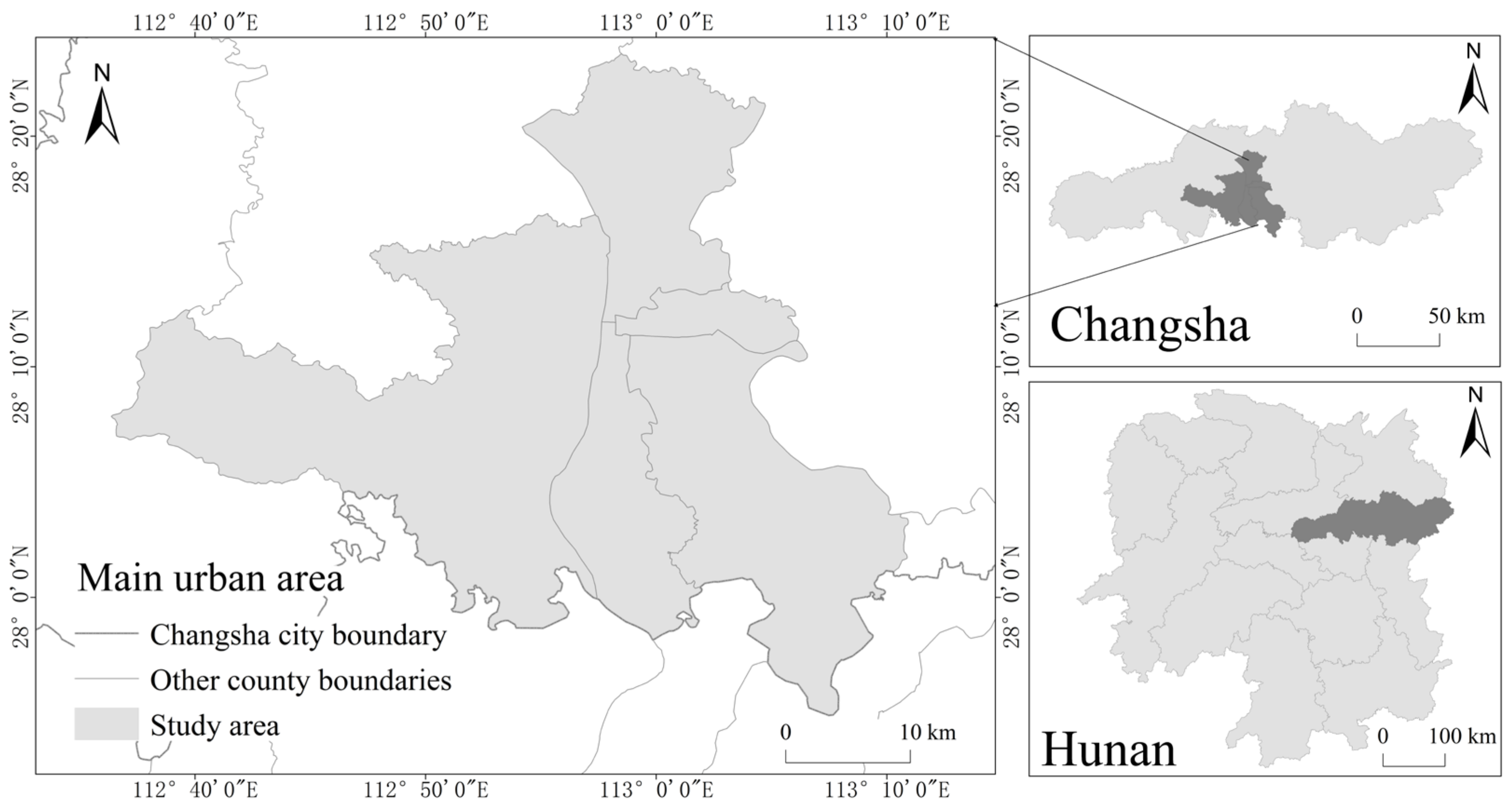
In this study, we have developed a comprehensive method for identifying inefficient urban land in the context of urban regeneration (Figure 1). The methodology consists of the following three main steps:
(1) Selection of indicators for characterizing urban land use efficiency: We carefully selected indicators specific to residential, commercial, and industrial land use. These indicators encompass multidimensional features such as building attribute, urban service, transportation condition, environmental quality, business performance, and production efficiency. The values of these indicators were derived from a diverse array of geographic big data sources. Following normalization and standardization, redundant indicators were eliminated using Spearman correlation analysis.
(2) Identification of urban inefficient land: The indicators derived from the first step were subjected to a hierarchical clustering method based on principal component analysis. This method partitions each of the three urban land categories into several clusters according to the similarity of land use characteristics. Subsequently, we identified clusters exhibiting inefficient utility characteristics as our identification results.
(3) Validation of inefficient land identification results: To verify the validity of our identification results, we conducted a random sampling of urban land followed by a field survey. We also calculated the kappa coefficient of the identification results to assess its accuracy.
Figure 1. Research flow.
Land 12 01957 g001

3.1. Study Area

Changsha, a representative city for rapid urbanization and implementation of inefficient urban land redevelopment policies in China [47], was selected as a case study for our method of identifying inefficient urban land. As the capital of Hunan Province and the leading city of the Chang-Zhu-Tan urban agglomeration, Changsha has experienced rapid urbanization in the past two decades. Its urbanization rate has risen from 53.87% in 2005 to 82.60% in 2021, and its built-up land area has expanded from 1306.12 km2 to 1953.31 km2. The study area covers the major urban administrative districts of Changsha, namely, Furong, Yuhua, Yuelu, Tianxin, and Kaifu Districts (Figure 2). These districts are the most dynamic and productive areas in Changsha in terms of economic development.
The current development pattern of the study area has been largely dominated by outward expansion [48], neglecting the social demands, environmental quality, public service provision, and cost-effective development in existing urban areas [49]. This has resulted in a significant amount of inefficient land within the main urban area, posing a serious challenge to the city’s high-quality development. In this study, we aim to provide scientific guidance for promoting a more intensive, efficient, and sustainable land use transition in Changsha by using it as a representative case study, thereby offering a reference for other cities.

3.2. Dataset

To conduct this study, we have collected and analyzed various types of data that reflect the urban morphology and human activity patterns of Changsha City. These data include high-resolution satellite imagery from Amap, street view imagery from Baidu Map Open Platform, points of interest (POI) data from Amap, road network data from OpenStreetMap (OSM), population heat map data from Baidu Map Open Platform, nighttime remote sensing imagery from Luojia-1A satellite, and evaluation data of various shops in Changsha City from a popular review website. Table 1 summarizes the sources, years, and interpretation of each type of data used in this paper.
We selected data from the period 2019 to 2022, taking into account the update frequency and timeliness of different data sources. Data such as satellite images, street view images, points of interest (POIs), and road networks reflect the city’s stable spatial structure and functional layout. Meanwhile, data such as population heat maps, nighttime lighting data, and store evaluations capture the city’s dynamic activities and economic benefits, necessitating timely updates. According to reports from the Changsha City Planning Bureau, Changsha has not undergone any major spatial changes since 2019, with the overall scale and structure of the city remaining stable [50,51]. Therefore, it is reasonable to select data in the time range of 2019–2022.
Furthermore, to enhance the spatial accuracy of the proposed method, we adopted different land use cells that reflect the spatial texture of the city as the research units. To achieve this, we implemented the following steps. Firstly, we used road network data from OpenStreetMap (OSM) to delineate the Traffic Analysis Zone (TAZ), which serves as a fundamental unit for urban planning. Secondly, we overlaid satellite images, Amap, and urban planning maps to identify and classify the land use units into residential, commercial, and industrial categories. Lastly, due to the difficulty of changing land ownership and the low demand for regeneration, we eliminated land use units that are irrelevant or incompatible with the method from the analysis, such as urban villages, vacant land, and land under construction.

3.3. Indicators for Measuring Land Use Efficiency

Urban space is a diverse and heterogeneous entity that reflects human activities and productivity in different land use types. Urban regeneration, a process of transforming urban space, involves different challenges and opportunities for different types of land use. In this study, we focus on three types of urban land use: residential, commercial, and industrial, because they are the main components of urban land use structure, and they have significant impacts on urban development, environment, and social welfare [52]. Residential land use provides the living environment for residents, which is influenced by the infrastructure provision, the housing quality, and the environmental conditions. Commercial land use supports economic activity, which is constrained by consumer demand, the built environment, and the location factors. Industrial land use drives the production process, which is affected by the building and equipment quality and resource efficiency.
To assess the characteristics of these three types of land use in Changsha, China, we selected 12, 11, and 5 indicators, respectively, based on the literature review and the geospatial data availability (Table 2). The selection of indicators is a critical step in the assessment process. We do not claim that our indicators are complete and exhaustive, but rather that they are representative and relevant for the purpose of our study.

3.3.1. Indicators for Residential Land

In the realm of residential land, indicators were selected from four key perspectives: building attribute, urban service, transportation condition, and environmental quality.
Building attribute comprises building condition (BC), building density (BD), and floor area ratio (FAR), which reflect the physical state and the spatial efficiency of the building. BC measures the year of completion of the building, which reflects the quality of the residential building [32]. BD is the ratio of building footprint area to land area, indicating the density of residential development [32]. FAR is the ratio of total building area to land area, indicating the intensity of residential development [32].
Urban service includes population density (PD), park accessibility (PA), commercial service coverage (CSC), and public service coverage (PSC), which reflect the living needs and convenience of the residents. PD is the number of people per unit area, indicating the population size and demand scale for infrastructures of residential land [12]. PA is the shortest time for residents to parks and squares, indicating the availability of recreation and outdoor activities of residential land [32,53]. CSC is the degree of clustering of commercial facilities, indicating the convenience of residents to access commercial services near their residential area [12,32]. PSC is the degree of clustering of public service facilities, such as education, healthcare, and culture, indicating the level of social welfare and public services that residents enjoy [12,32].
Transportation condition contains 400 m angular betweenness (4AB), 800 m angular betweenness (8AB), and 1200 m angular betweenness (12AB), which reflect the accessibility of the residential land. They represent the frequency of each road segment in the road network occurring on all shortest paths within 5, 10, and 15 min’ walking distance [54], respectively, reflecting the importance and traffic flow of the road segments. The higher the value of these indicators, the easier it is for residential sites to reach other locations and the more connected they are [32,54,55].
Environmental quality contains greenery (GR) and openness (OP), which are essential for the health and comfort of residents. GR refers to the proportion of the green area of the street in the field of view of the human eye, which reflects the greening and ecological quality of the residential land [56]. OP refers to the proportion of the sky of the street in the field of view of the human eye, which reflects the openness and comfort of the residential land [57].

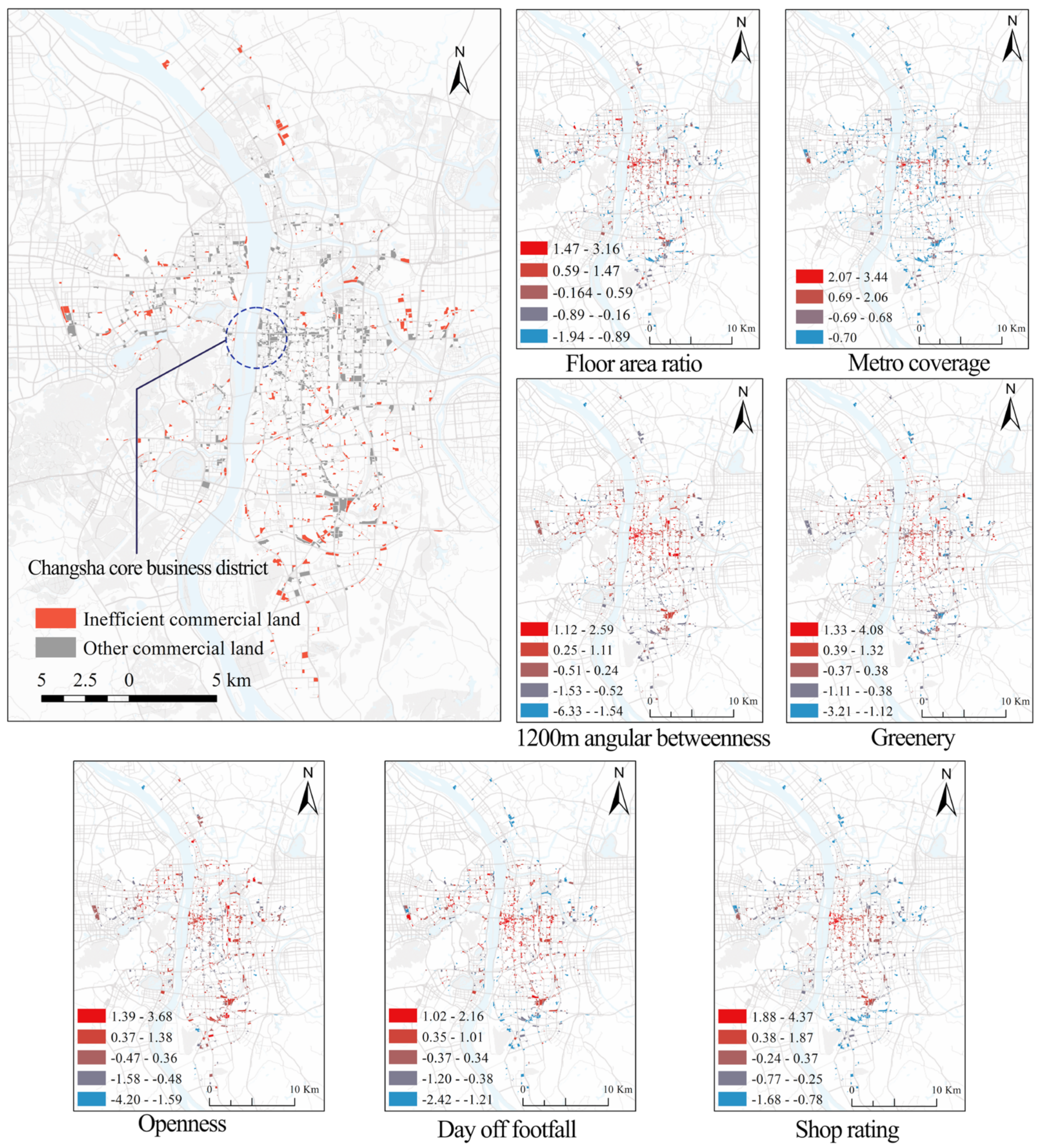
3.3.2. Indicators for Commercial Land

For commercial land, indicators were selected from four dimensions: building attribute, transportation condition, environmental quality, and business performance.
Building attribute refers to the FAR, which measures the total floor area of a building divided by the area of the land. FAR can indicate the development potential and utilization efficiency of commercial land [32].
Transportation condition includes metro coverage (MC), 4AB, 8AB, and 12AB. MC is the number of metro stations within a 500 m radius of the commercial land, reflecting the convenience and accessibility of the metro service [47,53,58]. 4AB, 8AB, and 12AB were used to assess the accessibility of the road network for commercial land [32,54,55].
Environmental quality contains GR and OP, which can help to assess the greenery and openness around the commercial land, which is essential for providing a comfortable shopping environment and attracting customers [56,57].
Business performance includes CSC, day off footfall (DF), weekday footfall (WF), and shop rating (SR), which can help to assess the economic activity and attractiveness of commercial land. CSC reflects the degree of concentration of commercial services [12,32,59], DF and WF reflect the patronage of a commercial site on days off and weekdays [32,60], and SR reflects the degree of business excellence of stores [61].

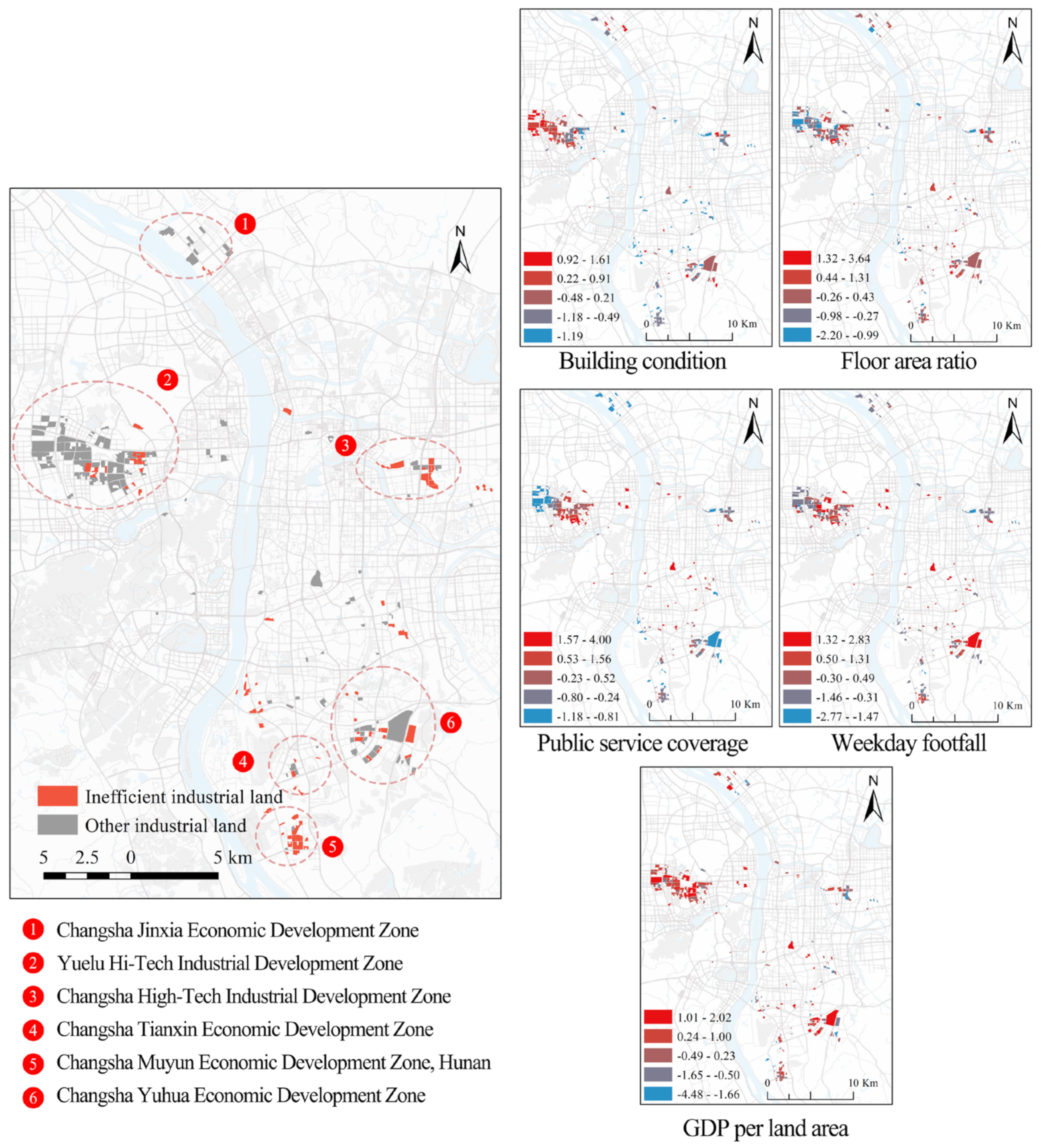
3.3.3. Indicators for Industrial Land

For industrial land, indicators were selected from three dimensions: building attribute, urban service, and production efficiency.
Building attribute includes BC and FAR, which reflects the physical characteristics and use of industrial land, and are the basic elements for evaluating the quality of industrial land. BC indicates the year of completion of the building, which reflects the state of the structure and maintenance of the industrial building [32]. FAR measures the total area of the building divided by the area of the land, reflecting the intensity of the utilization of the land [32].
Urban service includes PSC, which measures the level of public facilities and services available for industrial land, and it is an important factor affecting the attractiveness and sustainability of industrial land [12,32].
Production efficiency comprises WF and gross domestic product per land (GDP), which measure the economic contribution and development potential of industrial land. WF indicates the number of people visiting the industrial land during weekdays, reflecting the degree of activity and human resource supply of industrial land [32,60]. GDP measures the gross domestic product generated per unit area of industrial land, reflecting the productivity and added value of industrial land [26,27,62].

3.3.4. Measurement of Indicators

In this study, we employed multi-source data to measure various indicators of the city’s spatial quality, utilizing the following data processing methods: By consulting publicly available information on the Internet to obtain the year of completion for each type of building, we categorized the buildings by year into pre-1995, 1996–2000, 2001–2005, 2006–2010, 2011–2015, and post-2015, and we assigned a score of 1–6, respectively. The score is the BC value [32]. PD values were obtained by simulating population distribution using data from POI, night lighting, land use, road network, and DEM [63]. BD and FAR values were calculated in ArcGIS by extracting and mapping building outlines with reference to high-resolution satellite images. PA values were calculated by using the road network data and the road network analysis model of ArcGIS to estimate the shortest time of each parcel to the park and square entrances and exits [32,64]. The CSC and PSC values were obtained in ArcGIS by calculating the average kernel density of commercial POIs and public service POIs within each parcel, respectively [12,32]. 4AB, 8AB, and 12AB values were computed using sDNA tool to calculate the number of times each street is crossed by the shortest path between any two other street segments within a radius of 400, 800, and 1200 m, respectively [65]. Baidu Street View images and deep learning algorithms were used to calculate the proportion of green area and the proportion of sky area of the street in the human eye’s perspective in order to obtain the GR and OP value [66]. MC values were calculated by using the data of metro stations to calculate the number of accessible metro stations within 500 m of each plot. SR values were measured by using data from the Dianping website to calculate the weighted kernel density of shop ratings [61]. WF and DF values were measured by using Baidu heat map data to calculate the average 24 h heat value for a weekday and a rest day [60]. GDP values were calculated by simulating the spatial distribution of secondary and tertiary GDP using the Luojia-1A nighttime light images, obtained from Wuhan University, situated in Wuhan, China, and POI data [67].

3.4. Data Pre-Processing

We implemented data transformation and standardization techniques to address the skewness and kurtosis of the data and ensure the comparability of indicators within the method. This process involved analyzing quantile-quantile plots to assess the conformity of the data to a normal distribution. For variables exhibiting severe right-skewness, slight right-skewness, or left-skewness, we applied logarithmic, square root, or exponential transformations, respectively. Next, we scaled the data using z-score normalization, adjusting the mean and standard deviation of each indicator. To prevent collinearity among the data, we computed a Spearman correlation coefficient matrix for this study [68], and one of the indicators with a correlation coefficient greater than 0.80 was eliminated from the combination [43].

3.5. Principal Components Analysis

The principal component analysis (PCA) is a technique that reduces multicollinearity and the dimensionality of the data, using fewer variables to preserve as much of the original information about the study object as possible [69]. We utilized PCA to analyze the evaluation indicators for residential, commercial, and industrial land uses separately, aiming to simplify our metrics and facilitate easy interpretation. To ensure that the principal components capture as much original information as possible, we retained the principal components with a cumulative contribution of 70%. Moreover, we used the maximum variance of the eigenvectors for orthogonal rotation to improve the interpretive performance of the factor loadings.

3.6. Hierarchical Clustering Method

Hierarchical clustering in Python’s scikit-learn module [70] was used in this paper to identify clusters with inefficient land characteristics by grouping various types of lands based on the similarity of their principal components. In contrast to the divisive algorithm, which requires pre-defined criteria and procedures that might not fit reality or lose information, we chose the agglomerative hierarchical clustering algorithm, which can create various degrees of clusters based on how similar the data points are [71]. Therefore, we adopted the agglomerative hierarchical clustering algorithm in this paper. We computed a distance matrix between the retained PC values and used Euclidean distance and Ward’s aggregation method [72] to cluster. The optimal number of clusters was determined as the number of clusters corresponding to the maximum value of the silhouette coefficient, subject to the condition that the clustering results pass the significance test of the one-way ANOVA.

3.7. Accuracy Assessment of Identification Results

In order to evaluate the reliability of the proposed methodology, we conducted an empirical study in Changsha City with a sampling test. First, we set a 95% confidence level and randomly sampled each of the three types of lands. Then, we verified the identification results of the selected samples by field research. The validation rules mainly referred to the scope of renewal objects defined in the Changsha Urban Renewal Plan [49] and the Measures for the Management of Redevelopment of Low-Efficient Land in Changsha Development Zone [73], as follows:
  • Old residential areas built before 2005 and resettlement areas with inadequate facilities were categorized as inefficient residential land.
  • Large and medium-sized specialized markets, as well as low-rise or outdated commercial service areas, are classified as inefficient commercial land.
  • Factories with a high vacancy rate and outdated industrial buildings are recognized as inefficient industrial land.
Finally, a confusion matrix was constructed based on the results of the field study, and then the accuracy and kappa coefficient were calculated. A confusion matrix is a table used to evaluate the performance of a classification model that shows how the model’s predicted results for different categories compare to the true results. The accuracy indicates the proportion of parcels correctly identified to the total number of parcels, and the kappa coefficient measures the consistency of the identification results with the actual situation. The closer these two parameters are to 1, the higher the recognition accuracy is.

4. Results

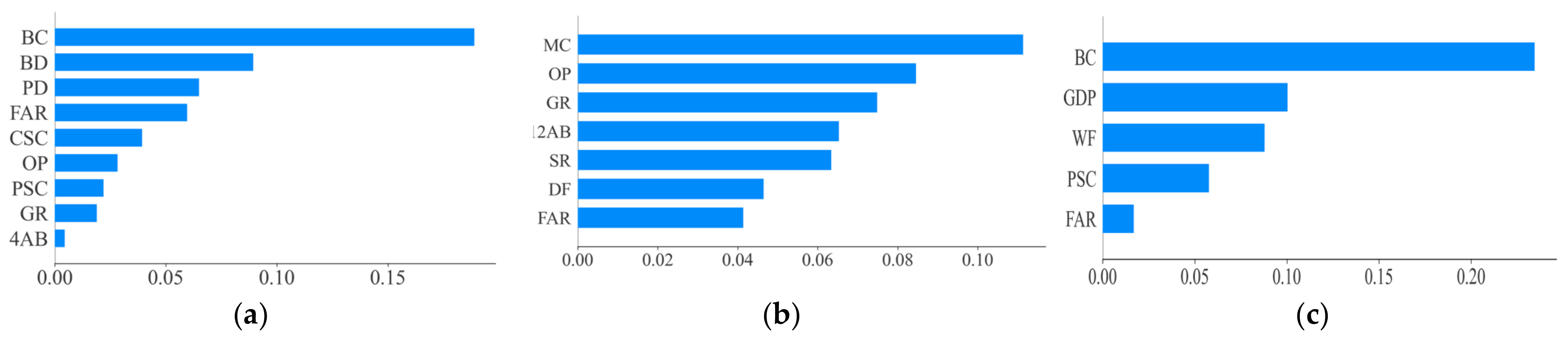
4.1. Filtering Results of Indicators for Characterizing Urban Land Use Efficiency

To analyze the interrelationships among the raw indicators, we calculated the Spearman correlation coefficients and visualized them in Figure 3. For residential land, a significant negative correlation of −0.82 was observed between PA and PD, indicating a trade-off between park accessibility and population density. Since PA shared similarities with CSC and PSP, which also assessed urban resource accessibility, we decided to eliminate PA from further analysis. Moreover, 4AB, 8AB, and 12AB were highly positively correlated with each other, with correlation coefficients above 0.8, indicating that any one of them was sufficient. We retained 4AB for this study. Regarding commercial land, we identified strong positive correlations between WF and DF (0.96), WF and SR (0.81), and CSC and SR (0.83). We chose to exclude WF and CSC as DF and SR served as more direct measures of the business performance of commercial land use. In addition, 4AB, 8AB, and 12AB were highly positively correlated with each other and any one of them was sufficient. We kept 12AB for this study. For industrial land, no notable correlations were found among the indicators, leading us to retain all of them for further analysis.

4.2. Principal Components of Indicators for Characterizing Urban Land Use Efficiency

The filtered indicators for each land use type were subjected to principal component analysis, transforming them into a set of linearly uncorrelated variables, namely, the principal components. We retained three principal components for each type of land use, as they accounted for a high proportion of the variance explained: 74.77% for residential land, 74.55% for commercial land, and 80.16% for industrial land (Table 3). To facilitate the interpretation of the factors, we applied a maximum variance orthogonal rotation method to the results of the principal component analysis. From the rotated factor loading table, we observed that each original variable had a high correlation with one of the extracted principal components, indicating that our extraction results were reasonable and could be analyzed in the next step of clustering.

4.3. Identification of Inefficient Lands

The principal components of each land use category were subjected to a hierarchical cluster analysis, which revealed that the optimal number of clusters for residential, commercial and industrial land was 4, respectively. A one-way ANOVA confirmed that the differences between the clusters were statistically significant for each indicator (p < 0.000; Table 4, Table 5 and Table 6). Hence, the mean values of the indicators for each cluster could be used to characterize the different types of land use.
The efficiency of residential land (Table 4) varied across the four clusters. Cluster 1 boasted the best BC and FAR, the smallest BD, and moderate scores on other criteria. This cluster likely corresponded to new residential areas with low-density, high-rise structures, and excellent built environments. Cluster 2 had the worst BC, the largest PD and BD, and lower FAR. This cluster implied older neighborhoods with low-rise buildings that face overcrowding and poorly built environments. It exhibited elevated CSC, PSC, and 4AB, which resulted from the intense demand for accommodation and the earlier urbanization of the region. Conversely, the lower GR and OP in this cluster suggested deterioration and deficiency in the communal environments. Considering these factors, cluster 2 could be regarded as inefficient residential land. Cluster 3 showed moderate values for most indicators, except for 4AB, GR, and OP, which were the highest, indicating that this cluster benefited from better accessibility and environmental quality. Thus, we did not consider this cluster as inefficient residential land. Cluster 4 exhibited the smallest average values for the majority of the indicators, suggesting that despite the limited provision of facilities, such land use can meet the diminished population pressure of the cluster, and the architectural conditions were superior, so it was not classified as inefficient land.
For commercial land (Table 5), cluster 2 manifested the lowest mean values for all indicators, indicating that this type of land use performed poorly in all aspects and could therefore be directly identified as inefficient commercial land. The other clusters each had the highest mean values for some indicators, while the rest of the indicators were in the middle range of values. Cluster 2 was the most consistent with the characteristics of inefficient commercial land.
The four clusters of industrial land (Table 6) exhibited significant differences in their indicators. Cluster 1 demonstrated the lowest average values for BC and GDP, as well as lower mean values for FAR, WF and PSC. This suggested that this cluster primarily consists of outdated plants and equipment, occupying extensive land areas, but suffered from low utilization rates and limited access to urban resources. Consequently, we classified this cluster as inefficient industrial land. Cluster 2 exhibited the highest average FAR value and higher values for BC, PSC, and WF. It is inferred that this cluster predominantly comprised new high-rise factory buildings, housing emerging industries that required less floor space and were situated closer to the city center. Cluster 3 was distinguished by the best building condition, with higher mean values for GDP. However, it performed poorly in FAR and PSC. This indicated that this cluster accommodated firms that needed large factory floor space and that they have built new factories on the urban fringe where land prices were low. Cluster 4 showed the highest mean values for PSC, WF, and GDP, implying that this cluster had the highest production capacity. Therefore, we did not classify Clusters 2, 3, and 4 as inefficient industrial land.

4.4. Spatial Distribution Pattern of Inefficient Lands

Based on the identification results, we obtained the spatial distribution of inefficient residential land, inefficient commercial land, and inefficient industrial land within the existing urban areas of Changsha.
The spatial distribution of inefficient residential land reveals a concentration in the city center, while a smaller portion is distributed at the city fringe, as depicted in Figure 4. This pattern indicates a trend of spreading from the city center to the city fringe. The total area of inefficient residential land measures 31.77 km2, accounting for 30.41% of the overall residential land area, as shown in Table 7. Numerous old residential districts and historic core neighborhoods can be found within the South Second Ring Road-Wanjiali Road-Trinity Avenue area, which is closer to the city center. These neighborhoods were constructed around 2000 or earlier and face various challenges [49,74]. Outdated and low-rise buildings, cramped and irregular layouts, and a lack of public and green spaces contribute to a degraded living environment. Despite their proximity to parks, commercial areas, and public services, the aging and deterioration of municipal facilities hinder residents’ access to quality urban services that meet their current needs. These neighborhoods have low livability standards and require urgent improvement as a consequence. Additionally, there are inefficient residential sites located on the outskirts of the city, where many resettlement estates are situated [74]. These areas suffer from underdevelopment and limited access to essential urban services such as education, healthcare, transportation, and entertainment. As a result, residents in these estates experience a low quality of life.
The spatial distribution of inefficient commercial land in Changsha showcases a notable contrast between the Wuyi Business District and other areas, as depicted in Figure 5. Wuyi Business District stands out as the city’s most vibrant and prosperous commercial zone, attracting a significant influx of people and resources. Due to limited land availability, it has evolved into a high-density and high-intensity integrated business area [75]. However, outside of this central core zone, commercial land exhibits a more dispersed pattern without clear clustering. It covers an area of 5.68 km2, representing 28.67% of the total commercial land area, as indicated in Table 7. These peripheral areas exhibit lower commercial vitality compared to large-scale shopping malls and commercial streets, primarily due to underdeveloped transport networks and pedestrian flow. We divided the identified commercial inefficient land into two types. The first type comprises specialized trade markets characterized by low-rise buildings and large floor areas. The second type includes old or low-rise commercial buildings. Both types exhibit low land use intensity and neglect environmental greening and aesthetics.
The urban fringe accommodates a significant portion of inefficient industrial land, which is concentrated in multiple industrial parks (Figure 6). These parks include Changsha National Hi-Tech Industrial Development Zone, Longping Hi-Tech Park, and Changsha Tianxin Economic Development Zone. Additionally, some inefficient industrial land is dispersed in parks near the Second Ring Road, Changsha Yuhua Economic Development Zone, and Kaifu Hi-Tech Industrial Development Zone. The total area of inefficient industrial land is 5.42 km2, comprising 24.70% of the total industrial land area (Table 7). This spatial distribution arises from the suburbanization of industries, wherein urban functions expand towards the outskirts due to urban growth [76], which occurs when urban development pushes other urban functions outwards and relocates industrial parks to the edge of cities. Moreover, inefficient industrial land tends to be characterized by older and less productive facilities, equipment, and environments. These areas exhibit low land use efficiency and even house idle plants. These factories occupy a significant amount of land resources without generating corresponding economic benefits.

4.5. Accuracy Assessment Result

We conducted an empirical study using the main urban area of Changsha City as a case study and validated the accuracy of the method by random sampling and field investigation methods, following the criteria for identifying inefficient land established in Chapter 2.7. The number of land parcels that were involved in the method computation for residential, commercial, and industrial land was 2174, 1250, and 276, respectively. To ensure a 95% confidence interval, 327, 295, and 161 parcels were randomly selected as test samples for each respective land use category.
Through comparative analysis and validation (Figure 7), as well as the calculation of the confusion matrix (Table 8), the accuracy rates of identifying residential, commercial, and industrial land were found to be 0.87, 0.91, and 0.84, respectively, all surpassing 0.8. These results demonstrate a high level of accuracy in the identification outcomes of the research method developed in this paper. Moreover, the kappa coefficients for identifying these three types of land use were 0.71, 0.77, and 0.68, respectively, all exceeding 0.6. This confirmed a substantial degree of consistency between the research findings and the actual situation, as well as the effectiveness of the result analysis conducted in this study.

5. Discussion

The experimental results demonstrate that the method performed well in detecting inefficient land within built-up urban environments. However, the specific causes and relative contributions of various factors that contributed to inefficient land remained unclear. To address this knowledge gap, we built a classification model based on Random Forest, using the labels of inefficient land and non-inefficient land as the dependent variable and the values of each indicator as the independent variables. The Random Forest algorithm is highly accurate and robust, and it shows superiority in data classification compared to other machine learning methods [77]. The accuracy of the model trained in this study was high, with AUC values of 0.98, 0.97, and 0.98 for residential, commercial, and industrial sites, respectively. To further interpret the model results, we employed the SHAP explainer, a powerful tool for interpreting complex machine learning models, to reveal the differential impacts of different indicators on inefficient land. The main results are as follows:
(1) For inefficient residential land, the indicators that have the most significant influence are building condition, building density, population density, and floor area ratio (Figure 8a). Building condition and floor area ratio have negative effects on land use efficiency, whereas building density and population density have positive effects (Figure 9a). Therefore, to redevelop inefficient residential land, urban planners should prioritize the improvement of housing quality and amenities, while respecting the historical and cultural heritage of older urban areas. This implies avoiding large-scale demolition and reconstruction, and instead focusing on the preservation and renovation of existing buildings. Moreover, the redevelopment should also address the living needs of the residents, by ensuring adequate provision of public services and facilities, such as schools, hospitals, shops and parks. This would increase the accessibility and convenience of the residents, as well as foster a sense of community and belonging.
(2) The efficiency of commercial land is primarily influenced by several key factors, namely, metro coverage, openness, and greenery, as illustrated in Figure 8b. These factors have negative effects on the efficiency of commercial land, as demonstrated in Figure 9b. Hence, to redevelop inefficient commercial land, urban planners should improve the accessibility and attractiveness of commercial activities. This can be achieved by increasing the metro coverage and connectivity of the commercial land, reducing the dependence on private vehicles, and enhancing the mobility and convenience of consumers. Furthermore, the redevelopment should focus on creating more green spaces, public areas, and urban design elements, improving the environmental quality and aesthetic appeal of the commercial land to attract more consumers.
(3) The issue of inefficient industrial land is primarily influenced by several key indicators, including the building condition, GDP per land, and workforce flow, as depicted in Figure 8c. These indicators have been shown to have a negative impact on industrial land efficiency, as demonstrated in Figure 9c. Based on these findings, the redevelopment of inefficient industrial land should prioritize renovating or demolishing outdated factory buildings and involve replacing low-end industries with green and high-end industries. This would improve the utilization of industrial land and generate economic benefits. However, the social elements of this redevelopment process should not be neglected, such as the workers’ livelihood and welfare. This includes ensuring fair compensation and relocation plans are in place, as well as investing in the enhancement of workers’ skills and education to prepare them for employment in new industries. Moreover, due respect should be given to preserving sites of industrial heritage, acknowledging their historical significance and value.

6. Conclusions

A novel method was proposed to identify inefficient land in existing urban areas of residential, commercial, and industrial land. To assess the characteristics of these land uses, we selected evaluating indicators from multi-dimensions, including building attribute, urban service, transportation conditions, environmental quality, business performance, and production efficiency, and then used multi-source geospatial data to measure these indicators. Then, we applied hierarchical clustering based on the principal components of these indicators to group the land use parcels into different categories and extracted the ones that exhibit inefficient land characteristics as the identification results.
The proposed model was conducted in the main urban area of Changsha City, and the results were compared with the ground truth to evaluate its effectiveness. The model accurately identified inefficient residential land, commercial land, and industrial land, showing a high level of agreement with reality, with kappa coefficients of 0.71, 0.77, and 0.68, respectively. The study revealed the spatial patterns of inefficient urban land in the city. The inefficient residential land is concentrated in the central area, where the old city is located, while it is dispersed in the peripheral area. The inefficient commercial land is relatively uniformly distributed across the city, except for the core commercial area, where it is less prevalent. The inefficient industrial land clusters towards the edge of the city, forming several agglomerations around industrial parks.
The proposed method advances the previous studies in three aspects: Firstly, while most preceding studies have employed a uniform indicator framework to assess various types of land use [12,32], this method adopts distinct indicator frameworks for different land use types, reflecting the inherent diversity and complexity of urban land use. Secondly, this method employs unsupervised machine learning techniques to determine indicator weights, minimizing subjective bias and enhancing scientific rigor and reliability, while the majority of existing studies have relied on subjective or semi-subjective methods [36,37]. Third, this method leverages geographic big data for quantitative evaluation, enabling efficient, large-scale assessments at a granular level, while the spatial accuracy of previous studies has typically been limited to administrative districts or homogenized grid cells [12,26,27,62], resulting in low spatial precision.
Despite these merits, our method has some limitations that require further research. One of the main drawbacks is that, due to the limitations of data collection, many important indicators will be ignored, such as residents’ perceptions, store revenues, and the actual labor input and profit of industrial land. This may result in the misidentification of villa areas, upscale commercial areas, and high-tech industrial areas as inefficient urban land. These areas may have low scores on some indicators, such as population density, building density, greening rate, etc., but they may also have high value and potential on other aspects, such as resident satisfaction, business vitality, and industrial innovation. Therefore, this method needs to be further refined and optimized to reduce the likelihood of misidentification and to enhance the accuracy and credibility of the identification results. Another limitation stems from the reliance of the method on multiple sources of geographic data. This enhances its applicability to other large cities but raises questions about its validity and reliability in small cities where spatial data coverage is sparse and incomplete. For example, some indicators, such as accessibility and public service facilities, may not be accurately measured or updated in small cities due to the lack of data sources or the low frequency of data collection. This may lead to the underestimation or overestimation of inefficient urban land in these areas and affect the comparability and generalizability of the results. Therefore, the method needs to be adapted and validated for different urban contexts and scales, and it needs to take into account the availability and quality of geographic data in different regions.

Author Contributions

Conceptualization, C.H., P.W. and R.J.; methodology, C.H.; validation, C.H.; formal analysis, C.H.; investigation, C.H.; data curation, C.H. and J.M.; writing—original draft preparation, C.H.; writing—review and editing, R.J. and Y.W.; visualization, C.H.; supervision, R.J. and Y.W.; project administration, R.J. and Y.W.; funding acquisition, R.J. and Y.W. All authors have read and agreed to the published version of the manuscript.

Funding

This research was funded by the National Natural Science Foundation of China (grant number: 42271486 and 42101438); Humanity and Social Science Youth foundation of Ministry of Education of China (grant number: 21YJCZH151 and 20YJC790055); Hunan Province Natural Science Foundation, China (grant number: 2022JJ30391); Changsha City Outstanding Innovation Youth Training Program, China (grant number: kq2206025); and funding for the Major Scientific and Technological Project of Hunan Provincial Department of Natural Resources in 2022: “Research on Key Technologies for Coordinated Implementation and Monitoring and Supervision of Territorial Spatial Planning in Hunan Province”.

Conflicts of Interest

The authors declare no conflict of interest.

References

  1. UN-Habitat. World Cities Report 2022; UN-Habitat: Nairobi, Kenya, 2022. [Google Scholar]
  2. Lu, L.; Guo, H.; Corbane, C.; Li, Q. Urban sprawl in provincial capital cities in China: Evidence from multi-temporal urban land products using Landsat data. Sci. Bull. 2019, 64, 955–957. [Google Scholar] [CrossRef]
  3. El Garouani, A.; Mulla, D.J.; El Garouani, S.; Knight, J. Analysis of urban growth and sprawl from remote sensing data: Case of Fez, Morocco. Int. J. Sustain. Built Environ. 2017, 6, 160–169. [Google Scholar] [CrossRef]
  4. Scolozzi, R.; Geneletti, D. A multi-scale qualitative approach to assess the impact of urbanization on natural habitats and their connectivity. Environ. Impact Assess. Rev. 2012, 36, 9–22. [Google Scholar] [CrossRef]
  5. Hasse, J.E.; Lathrop, R.G. Land resource impact indicators of urban sprawl. Appl. Geogr. 2003, 23, 159–175. [Google Scholar] [CrossRef]
  6. Shaker, R.R.; Altman, Y.; Deng, C.; Vaz, E.; Forsythe, K.W. Investigating urban heat island through spatial analysis of New York City streetscapes. J. Clean. Prod. 2019, 233, 972–992. [Google Scholar] [CrossRef]
  7. Holcombe, R.G.; Williams, D.W. Urban sprawl and transportation externalities. Rev. Reg. Stud. 2010, 40, 257–273. [Google Scholar] [CrossRef]
  8. Castellar, J.A.C.; Popartan, L.A.; Pueyo-Ros, J.; Atanasova, N.; Langergraber, G.; Säumel, I.; Corominas, L.; Comas, J.; Acuña, V. Nature-based solutions in the urban context: Terminology, classification and scoring for urban challenges and ecosystem services. Sci. Total Environ. 2021, 779, 146237. [Google Scholar] [CrossRef]
  9. Bibri, S.E.; Krogstie, J.; Kärrholm, M. Compact city planning and development: Emerging practices and strategies for achieving the goals of sustainability. Dev. Built Environ. 2020, 4, 100021. [Google Scholar] [CrossRef]
  10. Shrivastava, R.; Sharma, A. Smart Growth: A Modern Urban Principle. Archit. Res. 2012, 1, 8–11. [Google Scholar] [CrossRef]
  11. Frantzeskaki, N.; Broto, V.C.; Coenen, L.; Loorbach, D. (Eds.) Urban Sustainability Transitions; Routledge: London, UK, 2017. [Google Scholar]
  12. Han, B.; Jin, X.B.; Wang, J.X.; Yin, Y.X.; Liu, C.J.; Sun, R.; Zhou, Y.K. Identifying inefficient urban land redevelopment potential for evidence-based decision making in China. Habitat Int. 2022, 128, 102661. [Google Scholar] [CrossRef]
  13. United Nations Human Settlements Programme. Urban Regeneration. Available online: https://unhabitat.org/topic/urban-regeneration (accessed on 15 January 2023).
  14. Petzet, M.; Heilmeyer, F. Architecture as Resource; Hatje Cantz Verlag: Ostfildern, Berlin, 2012. [Google Scholar]
  15. Heidenreich, M. The New Museum Folkwang in Essen. A Contribution to the Cultural and Economic Regeneration of the Ruhr Area? Eur. Plan. Stud. 2015, 23, 1529–1547. [Google Scholar] [CrossRef]
  16. Balletto, G.; Ladu, M.; Camerin, F.; Ghiani, E.; Torriti, J. More Circular City in the Energy and Ecological Transition: A Methodological Approach to Sustainable Urban Regeneration. Sustainability 2022, 14, 14995. [Google Scholar] [CrossRef]
  17. Stein, S. (Ed.) Capital City: Gentrification and the Real Estate State; Verso: London, UK, 2019. [Google Scholar]
  18. Anguelovski, I.; Connolly, J.J. (Eds.) The Green City and Social Injustice; Routledge: London, UK, 2021. [Google Scholar]
  19. Bai, Y.; Zhou, W.; Guan, Y.; Li, X.; Huang, B.; Lei, F.; Yang, H.; Huo, W. Evolution of Policy Concerning the Readjustment of Inefficient Urban Land Use in China Based on a Content Analysis Method. Sustainability 2020, 12, 797. [Google Scholar] [CrossRef]
  20. Zhou, T.; Zhou, Y.L.; Liu, G.W. Key Variables for Decision-Making on Urban Renewal in China: A Case Study of Chongqing. Sustainability 2017, 9, 370. [Google Scholar] [CrossRef]
  21. Olshammar, G. Greenfields, brownfields & housing development. Eur. Plan. Stud. 2003, 11, 1006–1008. [Google Scholar]
  22. Zitti, M.; Ferrara, C.; Perini, L.; Carlucci, M.; Salvati, L. Long-Term Urban Growth and Land Use Efficiency in Southern Europe: Implications for Sustainable Land Management. Sustainability 2015, 7, 3359–3385. [Google Scholar] [CrossRef]
  23. Couch, C.; Fraser, C.; Percy, S. Urban Regeneration in Europe; John Wiley & Sons: Hoboken, NJ, USA, 2008. [Google Scholar]
  24. Ministry of Natural Resources of China. Notice of the Ministry of Land and Resources on Issuing the Guiding Opinions on Deepening the Redevelopment of Inefficient Land in Urban Areas (Trial) (Land and Resources Development No. 147 of 2016); Ministry of Natural Resources of China: Beijing, China, 2016. (In Chinese) [Google Scholar]
  25. Lu, X.; Zhang, Y.; Li, J.; Duan, K. Measuring the urban land use efficiency of three urban agglomerations in China under carbon emissions. Environ. Sci. Pollut. Res. 2022, 29, 36443–36474. [Google Scholar] [CrossRef]
  26. Liu, S.; Xiao, W.; Li, L.; Ye, Y.; Song, X. Urban land use efficiency and improvement potential in China: A stochastic frontier analysis. Land Use Policy 2020, 99, 105046. [Google Scholar] [CrossRef]
  27. Pang, Y.Y.; Wang, X.J. Land-Use Efficiency in Shandong (China): Empirical Analysis Based on a Super-SBM Model. Sustainability 2020, 12, 618. [Google Scholar] [CrossRef]
  28. Chen, Y.; Chen, Z.; Xu, G.; Tian, Z. Built-up land efficiency in urban China: Insights from the General Land Use Plan (2006–2020). Habitat Int. 2016, 51, 31–38. [Google Scholar] [CrossRef]
  29. Koroso, N.H.; Zevenbergen, J.A.; Lengoiboni, M. Urban land use efficiency in Ethiopia: An assessment of urban land use sustainability in Addis Ababa. Land Use Policy 2020, 99, 105081. [Google Scholar] [CrossRef]
  30. Pan, Y.; Tian, Y.; Liu, X.; Gu, D.; Hua, G. Urban Big Data and the Development of City Intelligence. Engineering 2016, 2, 171–178. [Google Scholar] [CrossRef]
  31. Goodchild, M.F. Citizens as sensors: The world of volunteered geography. GeoJournal 2007, 69, 211–221. [Google Scholar] [CrossRef]
  32. Liu, Y.; Zhu, A.X.; Wang, J.; Li, W.; Hu, G.; Hu, Y. Land-use decision support in brownfield redevelopment for urban renewal based on crowdsourced data and a presence-and-background learning (PBL) method. Land Use Policy 2019, 88, 104188. [Google Scholar] [CrossRef]
  33. Nagata, S.; Nakaya, T.; Hanibuchi, T.; Amagasa, S.; Kikuchi, H.; Inoue, S. Objective scoring of streetscape walkability related to leisure walking: Statistical modeling approach with semantic segmentation of Google Street View images. Health Place 2020, 66, 102428. [Google Scholar] [CrossRef]
  34. Tang, J.; Long, Y. Measuring visual quality of street space and its temporal variation: Methodology and its application in the Hutong area in Beijing. Landsc. Urban Plan. 2019, 191, 103436. [Google Scholar] [CrossRef]
  35. Goodchild, M.F. The quality of big (geo)data. Dialogues Hum. Geogr. 2013, 3, 280–284. [Google Scholar] [CrossRef]
  36. Cui, G.; Zheng, W.; Chen, S.; Dong, Y.; Huang, T. Study on the Spatial Pattern Characteristics and Influencing Factors of Inefficient Urban Land Use in the Yellow River Basin. Land 2022, 11, 1562. [Google Scholar] [CrossRef]
  37. Wedding, G.C.; Crawford-Brown, D. Measuring site-level success in brownfield redevelopments: A focus on sustainability and green building. J. Environ. Manag. 2007, 85, 483–495. [Google Scholar] [CrossRef]
  38. Tarekegn, A.N.; Michalak, K.; Giacobini, M. Cross-Validation Approach to Evaluate Clustering Algorithms: An Experimental Study Using Multi-Label Datasets. SN Comput. Sci. 2020, 1, 263. [Google Scholar] [CrossRef]
  39. Ran, X.J.; Zhou, X.B.; Lei, M.; Tepsan, W.; Deng, W. A Novel K-Means Clustering Algorithm with a Noise Algorithm for Capturing Urban Hotspots. Appl. Sci. 2021, 11, 11202. [Google Scholar] [CrossRef]
  40. Tang, W.; Pi, D.C.; He, Y. A Density-Based Clustering Algorithm with Sampling for Travel Behavior Analysis. In Proceedings of the Intelligent Data Engineering and Automated Learning-Ideal 2016, Yangzhou, China, 12–14 October 2016; pp. 231–239. [Google Scholar]
  41. Ma, X.L.; Zuo, H.; Tian, M.J.; Zhang, L.Y.; Meng, J.; Zhou, X.N.; Min, N.; Chang, X.Y.; Liu, Y. Assessment of heavy metals contamination in sediments from three adjacent regions of the Yellow River using metal chemical fractions and multivariate analysis techniques. Chemosphere 2016, 144, 264–272. [Google Scholar] [CrossRef]
  42. Shahriar, N.; Faisal, S.M.A.A.; Pinjor, M.M.; Rafi, M.A.S.Z.; Sarkar, A.R. Comparative Performance Analysis of K-Means and DBSCAN Clustering algorithms on various platforms. In Proceedings of the 2019 22nd International Conference on Computer and Information Technology (ICCIT), Dhaka, Bangladesh, 18–20 December 2019; pp. 1–6. [Google Scholar]
  43. Lemoine-Rodriguez, R.; Inostroza, L.; Zepp, H. The global homogenization of urban form. An assessment of 194 cities across time. Landsc. Urban Plan. 2020, 204, 103949. [Google Scholar] [CrossRef]
  44. Xu, S.; Xu, S.S.; Ye, N.; Zhu, F. Automatic extraction of street trees’ nonphotosynthetic components from MLS data. Int. J. Appl. Earth Obs. Geoinf. 2018, 69, 64–77. [Google Scholar] [CrossRef]
  45. Rodriguez, J.; Semanjski, I.; Gautama, S.; Van de Weghe, N.; Ochoa, D. Unsupervised Hierarchical Clustering Approach for Tourism Market Segmentation Based on Crowdsourced Mobile Phone Data. Sensors 2018, 18, 2972. [Google Scholar] [CrossRef] [PubMed]
  46. Richards, D.R.; Tuncer, B. Using image recognition to automate assessment of cultural ecosystem services from social media photographs. Ecosyst. Serv. 2018, 31, 318–325. [Google Scholar] [CrossRef]
  47. Ministry of Natural Resources of China. Notice on Carrying out the Pilot Work of Redevelopment of Inefficient Land; Ministry of Natural Resources of China: Beijing, China, 2023. (In Chinese) [Google Scholar]
  48. Tan, X.; Ouyang, Q.; Jiang, Z.; Liu, Z.; Tan, J.; Zhou, G. Urban Spatial Expansion and Its Influence Factors Based on RS/GIS:A Case Study in Changsha. Econ. Geogr. 2017, 37, 81–85. (In Chinese) [Google Scholar] [CrossRef]
  49. Changsha Natural Resources and Planning Bureau. Changsha Urban Renewal Special Plan (2021–2035) (Draft for Public Comment); Changsha Natural Resources and Planning Bureau: Changsha, China, 2021. (In Chinese)
  50. Changsha Natural Resources and Planning Bureau. Changsha City Master Plan (2003–2020) (Revised in 2014); Changsha Natural Resources and Planning Bureau: Changsha, China, 2014. (In Chinese)
  51. Changsha Natural Resources and Planning Bureau. Changsha City Spatial Planning (2021–2035) (Public Version); Changsha Natural Resources and Planning Bureau: Changsha, China, 2021. (In Chinese)
  52. Nuissl, H.; Siedentop, S. Urbanisation and Land Use Change. In Sustainable Land Management in a European Context: A Co-Design Approach; Weith, T., Barkmann, T., Gaasch, N., Rogga, S., Strauß, C., Zscheischler, J., Eds.; Springer International Publishing: Cham, Switzerland, 2021; pp. 75–99. [Google Scholar]
  53. Dou, Z.; Qiu, W.; Li, W.; Luo, D. Evaluation Process of Urban Spatial Quality and Utility Trade-Off for Post-COVID Working Preferences. In Proceedings of the Hybrid Intelligence, Singapore, 4 April 2023; pp. 223–232. [Google Scholar]
  54. Li, Y.; Yabuki, N.; Fukuda, T. Integrating GIS, deep learning, and environmental sensors for multicriteria evaluation of urban street walkability. Landsc. Urban Plan. 2023, 230, 104603. [Google Scholar] [CrossRef]
  55. Humphries, H.C.; Bourgeron, P.S.; Reynolds, K.M. Sensitivity Analysis of Land Unit Suitability for Conservation Using a Knowledge-Based System. Environ. Manag. 2010, 46, 225–236. [Google Scholar] [CrossRef] [PubMed]
  56. Ye, Y.; Richards, D.; Lu, Y.; Song, X.; Zhuang, Y.; Zeng, W.; Zhong, T. Measuring daily accessed street greenery: A human-scale approach for informing better urban planning practices. Landsc. Urban Plan. 2019, 191, 103434. [Google Scholar] [CrossRef]
  57. Gong, F.-Y.; Zeng, Z.-C.; Zhang, F.; Li, X.; Ng, E.; Norford, L.K. Mapping sky, tree, and building view factors of street canyons in a high-density urban environment. Build. Environ. 2018, 134, 155–167. [Google Scholar] [CrossRef]
  58. Chrysochoou, M.; Brown, K.; Dahal, G.; Granda-Carvajal, C.; Segerson, K.; Garrick, N.; Bagtzoglou, A. A GIS and indexing scheme to screen brownfields for area-wide redevelopment planning. Landsc. Urban Plan. 2012, 105, 187–198. [Google Scholar] [CrossRef]
  59. Zhao, Z.; Zheng, X.; Fan, H.; Sun, M. Urban spatial structure analysis: Quantitative identification of urban social functions using building footprints. Front. Earth Sci. 2021, 15, 507–525. [Google Scholar] [CrossRef]
  60. Min, Z.; Ding, F. Analysis of Temporal and Spatial Distribution Characteristics of Street Vitality Based on Baidu Thermal Diagram: The Case of the Historical City of Nanchang City, Jiangxi Province. Urban Dev. Stud. 2020, 27, 31–36. (In Chinese) [Google Scholar]
  61. Qin, X.; Zhen, F.; Zhu, S.; Xi, G. Spatial Pattern of Catering Industry in Nanjing Urban Area Based on the Degree of Public Praise from Internet: A Case Study of Dianping.com. Sci. Geogr. Sin. 2014, 34, 810–817. (In Chinese) [Google Scholar] [CrossRef]
  62. Li, S.; Fu, M.; Tian, Y.; Xiong, Y.; Wei, C. Relationship between Urban Land Use Efficiency and Economic Development Level in the Beijing–Tianjin–Hebei Region. Land 2022, 11, 976. [Google Scholar] [CrossRef]
  63. Ma, Y.; Li, D.; Zhou, L.; Zhang, D.; Wang, J. The Spatial Accessibility and Matching Degree between the Supply and Demand of Basic Educational Resources in Changsha City. Trop. Geogr. 2021, 41, 1060–1072. (In Chinese) [Google Scholar] [CrossRef]
  64. ArcGIS Desktop: Release 10.8.1; Environmental Systems Research Institute: Redlands, CA, USA, 2020.
  65. Cooper, C.H.V.; Chiaradia, A.J.F. sDNA: 3-d spatial network analysis for GIS, CAD, Command Line-Python. SoftwareX 2020, 12, 100525. [Google Scholar] [CrossRef]
  66. Yao, Y.; Liang, Z.T.; Yuan, Z.H.; Liu, P.H.; Bie, Y.P.; Zhang, J.B.; Wang, R.Y.; Wang, J.L.; Guan, Q.F. A human-machine adversarial scoring framework for urban perception assessment using street-view images. Int. J. Geogr. Inf. Sci. 2019, 33, 2363–2384. [Google Scholar] [CrossRef]
  67. Zhang, A.; Pan, Y.; Ming, Y.; Wang, J. Research of GDP Spatialization based on Multisource Information Coupling: A Case Study in Beijing. Remote Sens. Technol. Appl. 2021, 36, 463–472. (In Chinese) [Google Scholar]
  68. Spearman, C. The proof and measurement of association between two things. By C. Spearman, 1904. Am. J. Psychol. 1987, 100, 441–471. [Google Scholar] [CrossRef]
  69. Kaiser, H.F. The application of electronic computers to factor analysis. Educ. Psychol. Meas. 1960, 20, 141–151. [Google Scholar] [CrossRef]
  70. Pedregosa, F.; Varoquaux, G.; Gramfort, A.; Michel, V.; Thirion, B.; Grisel, O.; Blondel, M.; Prettenhofer, P.; Weiss, R.; Dubourg, V.; et al. Scikit-learn: Machine learning in Python. J. Mach. Learn. Res. 2011, 12, 2825–2830. [Google Scholar]
  71. Roux, M. A Comparative Study of Divisive and Agglomerative Hierarchical Clustering Algorithms. J. Classif. 2018, 35, 345–366. [Google Scholar] [CrossRef]
  72. Murtagh, F.; Legendre, P. Ward’s Hierarchical Agglomerative Clustering Method: Which Algorithms Implement Ward’s Criterion? J. Classif. 2014, 31, 274–295. [Google Scholar] [CrossRef]
  73. Government of China. Measures for the Management of Redevelopment of Low-Efficienct Land in Changsha Development Zone; Government of China: Changsha, China, 2019; pp. 1–5. (In Chinese)
  74. Jiang, L.; Feng, C. The Study of Residential Differentiation in ChangshaBased on the Social-Spatial Perspective. Econ. Geogr. 2015, 35, 78–86. (In Chinese) [Google Scholar] [CrossRef]
  75. Ye, Q.; Zhao, Y.; Hu, Z.; Pan, R. Research on Ratail Commercial Space Agglomeration and Its Influencing Mechanism Based on Spatial Heterogeneity: A Case Study of Changsha. Mod. Urban Res. 2021, 1, 52–58. (In Chinese) [Google Scholar]
  76. Zhang, L.; Yue, W.; Liu, Y.; Fan, P.; Wei, Y.D. Suburban industrial land development in transitional China: Spatial restructuring and determinants. Cities 2018, 78, 96–107. [Google Scholar] [CrossRef]
  77. Hassan, C.A.U.; Khan, M.S.; Shah, M.A. Comparison of Machine Learning Algorithms in Data classification. In Proceedings of the 2018 24th International Conference on Automation and Computing (ICAC), Newcastle University, UK, 6–7 September 2018; pp. 1–6. [Google Scholar]
Figure 2. Location map of the study area.
Land 12 01957 g002
Figure 3. Correlation coefficient matrices. (a) Correlation coefficient matrix for residential land; (b) Correlation coefficient matrix for commercial land; (c) Correlation coefficient matrix for industrial land (Darker blue indicates a higher correlation coefficient and the lighter blue indicates a lower correlation coefficient).
Land 12 01957 g003
Figure 4. Distribution of inefficient residential land and indicator values for residential land (z-score).
Land 12 01957 g004
Figure 5. Distribution of inefficient commercial land and indicator values for commercial land (z-score).
Land 12 01957 g005
Figure 6. Distribution of inefficient industrial land and indicator values for industrial land (z-score).
Land 12 01957 g006
Figure 7. Typical examples of non-inefficient and inefficient land.
Land 12 01957 g007
Figure 8. Average impact on output magnitude. (a) Average impact on output magnitude for inefficient residential land; (b) Average impact on output magnitude for inefficient commercial land; (c) Average impact on output magnitude for inefficient industrial land.
Land 12 01957 g008
Figure 9. Impact on model output. (a) Impact on model output for inefficient residential land; (b) Impact on model output for inefficient commercial land; (c) Impact on model output for inefficient industrial land.
Land 12 01957 g009
Table 1. Description of data sources.
Data TypeData SourcesYearData Interpretation
High-resolution satellite imageryAmap (www.amap.com, accessed on 10 November 2021)2019It enables a synoptic observation of the city’s spatial structure and land use patterns.
Street View ImagesBaidu Maps Open Platform (https://lbsyun.baidu.com, accessed on 5 June 2022)2019It provides a detailed representation of the city’s urban morphology and architectural characteristics.
POIAmap (www.amap.com, accessed on 10 November 2021)2020It identifies the location and category of different urban functions and services.
Road networkOpenStreetMap (www.openstreetmap.org, accessed on 1 April 2022)2022It depicts the distribution of urban roads.
Population heat mapBaidu Maps Open Platform (https://lbsyun.baidu.com, accessed on 18 September 2022)2022It depicts the spatial distribution and intensity of human activity in the city.
Nighttime light dataNight remote sensing image products from Luojia-1A satellite (http://59.175.109.173:8888/app/login.html, accessed on 1 September 2022)2022It measures the city’s luminosity and energy consumption at night
Shop evaluation dataDianping (https://www.dianping.com, accessed on 1 January 2023)2022It evaluates the public perception and satisfaction with different urban amenities.
Table 2. Indicators for characterizing urban land use efficiency.
Type of LandIndicator (Indicator C Ode)Explanation
Residential landBuilding condition (BC)Year of completion of the building.
Building density (BD) D B = A i A
where A i is the base area of the building in unit i and A is the total area of the study area.
Floor area ratio (FAR) F A R = A i H i A
where A i is the base area of building i , H i is the number of floors of the building in the unit, and A is the total area of the study area.
Population density (PD) P D = p i A
where p i is the number of people in the unit and A is the total area of the study area.
Park accessibility (PA)The shortest time for land unit to parks and squares in ArcGIS.
Commercial service coverage (CSC)Kernel density calculation formula:
f ^ h x = 1 n h i = 1 n   K x x i h
where h is the bandwidth, n is the number of input elements, and K x is the kernel function.
Public service coverage (PSC)
400 m angular betweenness (4AB) b e t w e e n n e s s = y N z R y O D x , y , z W z P z t o t a l   w e i g h t y  
O D x , y , z = 1 , if x is on the first geodesic found from y to z ; 1 / 2 , x = y z ; 1 / 2 , x = z y ; 1 / 3 , x = z = y ; 0 , otherwise .
where N is the set of all road segments in the study area; R y is the set of other road segments reachable from road segment y within a given radius R (400 m, 800 m, or 1200 m); W z is the weight of road segment z; P z denotes the proportion of road segment z in R y ; t o t a l   w e i g h t y denotes the total weight of all road segments from road segment y within a given radius R.
800 m angular betweenness (8AB)
1200 m angular betweenness (12AB)
Greenery (GR) G R = g r e e n i i m a g e
where g r e e n i is the total area of tree, flower, and grass in unit i and i m a g e is the total area of the image.
Openness (OP) O P = s k y i i m a g e
where s k y i is the total area of the sky in unit i and i m a g e is the total area of the image.
Commercial landFloor area ratio (FAR) F A R = A i H i A
where A i is the base area of building i , H i   is the number of floors of the building in the unit, and A is the total area of the study area.
Metro coverage (MC)Number of accessible metro stations within 500 m of the unit.
400 m angular betweenness (4AB) b e t w e e n n e s s = y N z R y O D x , y , z W z P z t o t a l   w e i g h t y  
O D x , y , z = 1 , if x is on the first geodesic found from y to z ; 1 / 2 , x = y z ; 1 / 2 , x = z y ; 1 / 3 , x = z = y ; 0 , otherwise .
where N is the set of all road segments in the study area; R y is the set of other road segments reachable from road segment y within a given radius R (400 m, 800 m, or 1200 m); W z is the weight of road segment z; P z denotes the proportion of road segment z in R y ; t o t a l   w e i g h t y denotes the total weight of all road segments from road segment y within a given radius R.
800 m angular betweenness (8AB)
1200 m angular betweenness (12AB)
Greenery (GR) G R = g r e e n i i m a g e
where g r e e n i is the total area of tree, flower, and grass in unit i , i m a g e is the total area of the image.
Openness (OP) O P = s k y i i m a g e
where s k y i is the total area of the sky in unit i , i m a g e is the total area of the image.
Commercial service coverage (CSC)Kernel density calculation formula:
f ^ h x = 1 n h i = 1 n   K x x i h
where h is the bandwidth, n is the number of input elements, K x is the kernel function.
Day off footfall (DF) D F , W F = t = 1 m F t 24
where F t is the footfall in the unit t and m is the total hours of the day.
Weekday footfall (WF)
Shop rating (SR)Kernel density calculation formula:
f ^ h x = 1 n h i = 1 n   R i K x x i h
where h is the bandwidth, n is the number of input elements, K x is the kernel function, and R i is the score of shop i from the public.
Industrial landBuilding condition (BC)Year of completion of the building.
Floor area ratio (FAR) F A R = A i H i A
where A i is the base area of building i , H i   is the number of floors of the building in the unit, and A is the total area of the study area.
Public service coverage (PSC)Kernel density calculation formula:
f ^ h x = 1 n h i = 1 n   K x x i h
where h is the bandwidth, n is the number of input elements, K x is the kernel function.
Weekday footfall (WF) D F , W F = t = 1 m F t 24
where F t is the footfall in the unit t , m is the total hours of the day.
GDP per land (GDP) G D P = G D P i A
where G D P i is the number of people in the unit, A is the total area of the study area.
Table 3. PCs’ eigenvalues, explained, and cumulative variance and factor loadings after varimax rotation.
Type of LandEigenvectorsPC1PC2PC3
Residential landEigenvalue3.111.731.88
Variability (%)34.6019.2320.94
Cumulative (%)34.6053.8474.77
Factor loadings
Building condition (BC)−0.320.85−0.04
Population density (PD)0.86−0.230.16
Building density (BD)0.50−0.610.09
Floor area ratio (FAR)0.350.750.03
Commercial service coverage (CSC)0.88−0.120.20
Public service coverage (PSC)0.840.070.04
400 m angular betweenness (4AB)0.62−0.010.47
Greenery (GR)0.19−0.110.86
Openness (OP)0.080.060.92
Commercial landEigenvalue1.901.751.57
Variability (%)27.0825.0722.40
Cumulative (%)27.0852.1574.55
Factor loadings
Floor area ratio (FAR)0.880.01−0.01
Greenery (GR)0.150.83−0.03
Openness (OP)0.020.850.12
Metro coverage (MC)0.09−0.010.90
1200 m angular betweenness (12AB)0.540.510.40
Day off footfall (DF)0.640.210.52
Shop rating (SR)0.630.220.56
Industrial landEigenvalue1.821.141.05
Variability (%)36.3322.8021.03
Cumulative (%)36.3359.1380.16
Factor loadings
Building condition (BC)−0.150.890.16
Floor area ratio (FAR)0.180.120.92
Public service coverage (PSC)0.76−0.290.27
Weekday footfall (WF)0.84−0.080.20
GDP per land area (GDP)0.700.50−0.28
Table 4. ANOVA and descriptive statistics for residential land evaluation indicators by cluster.
Cluster
1 (Non-Inefficient)2 (Inefficient)3 (Non-Inefficient)4 (Non-Inefficient)
IndicatorsF ValueMin (Mean) MaxMin (Mean) MaxMin (Mean) MaxMin (Mean) Max
Building condition (BC)889.04−1.17 (0.86) 1.66−1.17 (−0.84) 1.66−1.17 (0.24) 1.66−1.17 (−0.2) 1.66
Population density (PD)307.31−2.08 (−0.28) 2.94−1.32 (0.62) 3.0−1.84 (−0.2) 2.25−2.08 (−1.12) 0.35
Building density (BD)411.32−2.84 (−0.66) 2.75−2.28 (0.72) 4.09−2.3 (−0.16) 2.1−2.02 (−0.18) 2.61
Floor area ratio (FAR)394.7−2.21 (0.71) 3.49−2.8 (−0.37) 2.5−2.8 (−0.02) 3.34−2.82 (−1.14) 0.94
Commercial service coverage (CSC)362.68−3.15 (−0.18) 2.52−2.16 (0.56) 2.68−2.43 (−0.08) 1.58−4.15 (−1.47) 0.16
Public service coverage (PSC)242.66−2.42 (0.03) 2.84−1.91 (0.4) 2.99−1.93 (−0.22) 2.23−2.95 (−1.39) 0.65
400m angular betweenness (4AB)174.61−2.97 (−0.21) 3.09−2.99 (0.31) 3.08−1.93 (0.38) 2.22−3.76 (−1.13) 0.65
Greenery (GR)496.53−2.09 (−0.41) 1.52−1.89 (0.04) 2.94−0.66 (1.31) 3.89−2.86 (−0.84) 1.22
Openness (OP)483.89−2.92 (−0.25) 1.89−2.43 (−0.13) 2.66−0.67 (1.36) 3.46−3.79 (−0.88) 1.99
Table 5. ANOVA and descriptive statistics for commercial land evaluation indicators by cluster.
Cluster
1 (Non-Inefficient)2 (Inefficient)3 (Non-Inefficient)4 (Non-Inefficient)
IndicatorsF ValueMin (Mean) MaxMin (Mean) MaxMin (Mean) MaxMin (Mean) Max
Floor area ratio (FAR)205.88−1.81 (0.16) 2.92−1.87 (−0.51) 1.87−1.94 (−0.34) 2.43−0.24 (1.18) 3.16
Greenery (GR)218.76−1.72 (−0.08) 2.0−3.21 (−0.66) 1.88−1.02 (0.97) 4.08−1.78 (0.27) 2.89
Openness (OP)201.19−1.64 (0.05) 2.43−4.2 (−0.64) 1.11−1.42 (0.97) 3.68−1.65 (−0.02) 2.74
Metro coverage (MC)707.24−0.7 (1.16) 3.44−0.7 (−0.62) 0.68−0.7 (−0.38) 0.68−0.7 (−0.57) 0.68
1200m angular betweenness (12AB)132.81−2.85 (0.41) 2.59−6.33 (−0.7) 1.38−1.84 (0.22) 2.16−1.75 (0.35) 2.18
Day off footfall (DF)181.37−1.84 (0.58) 2.16−2.42 (−0.69) 1.38−2.05 (−0.17) 1.93−1.76 (0.48) 2.13
Shop rating (SR)141.21−1.11 (0.6) 4.37−1.68 (−0.61) 0.99−1.28 (−0.18) 2.62−1.18 (0.29) 3.54
Table 6. ANOVA and descriptive statistics for industrial land evaluation indicators by cluster.
Cluster
1 (Non-Inefficient)2 (Inefficient)3 (Non-Inefficient)4 (Non-Inefficient)
IndicatorsF ValueMin (Mean) MaxMin (Mean) MaxMin (Mean) MaxMin (Mean) Max
Building condition (BC)129.4−1.19 (−0.74) 0.91−1.19 (0.76) 1.61−0.49 (0.87) 1.61−1.19 (−0.61) 0.91
Floor area ratio (FAR)102.63−2.2 (−0.12) 2.0−0.24 (1.51) 3.64−2.05 (−0.65) 0.93−1.43 (−0.21) 0.75
Public service coverage (PSC)62.23−1.13 (−0.18) 2.28−1.08 (0.46) 2.59−1.18 (−0.68) 1.16−0.47 (1.21) 4.0
Weekday footfall (WF)31.08−2.77 (−0.31) 2.34−1.0 (0.42) 2.36−2.28 (−0.36) 2.83−0.31 (0.99) 2.12
GDP per land area (GDP)29.56−4.48 (−0.6) 1.08−2.61 (0.17) 2.02−0.91 (0.35) 1.77−0.67 (0.66) 1.62
Table 7. Area of inefficient land by type and its share.
Type of LandInefficient Residential LandInefficient Commercial LandInefficient Industrial Land
Area (km2)30.355.685.53
Percentage (%)26.55%28.67%25.21%
Table 8. Parameters calculated from the confusion matrix.
Inefficient Residential LandInefficient Commercial LandInefficient Industrial Land
Predicted Value
PositiveNegativePositiveNegativePositiveNegative
Actual valuePositive843565185613
Negative620292031280
Accuracy0.870.910.84
Kappa coefficient0.710.770.68
Disclaimer/Publisher’s Note: The statements, opinions and data contained in all publications are solely those of the individual author(s) and contributor(s) and not of MDPI and/or the editor(s). MDPI and/or the editor(s) disclaim responsibility for any injury to people or property resulting from any ideas, methods, instructions or products referred to in the content.

