Optimizing Soil Moisture Retrieval: Utilizing Compact Polarimetric Features with Advanced Machine Learning Techniques

Abstract

Soil moisture plays a crucial role in various environmental processes and is essential for agricultural management, hydrological modeling, and climate studies. Synthetic Aperture Radar (SAR) remote sensing presents significant potential for estimating soil moisture due to its ability to operate in all weather conditions and provide day-and-night imaging capabilities. Among the SAR configurations, the Compact Polarimetric (CP) mode has gained increasing interest as it relaxes system constraints, improves coverage, and enhances target information compared to conventional dual polarimetric SAR systems. This paper introduces a novel approach for soil moisture retrieval utilizing machine learning algorithms and CP SAR features. The CP SAR features are derived from a series of RADARSAT Constellation Mission (RCM) CP SAR imagery acquired over Canadian experimental sites equipped with Real-Time In Situ Soil Monitoring for Agriculture (RISMA) stations. This study employs a diverse dataset of compact polarimetric SAR features and corresponding ground truth soil moisture measurements for training and validation purposes. The results of our study achieved a Root Mean Square Error (RMSE) of 6.88% with a coefficient of determination R² equal to 0.60, which corresponds to a correlation R between true and predicted soil moisture values of 0.75, using optimized Ensemble Learning Regression (ELR) with a decision-tree-based model. These results improved, yielding an RMSE of 5.67% and an R² equal to 0.73 (R = 0.85), using an optimized Gaussian Process Regression (GPR) model.

1. Introduction

Synthetic Aperture Radar (SAR) has emerged as a compelling technology for high-resolution soil moisture content observation [1,2,3,4]. SAR remote sensing has been utilized in soil moisture retrieval using either conventional single, dual [1], or full polarimetric SAR imagery [4]. The observation of temporal and spatial patterns of soil moisture holds significant importance for agriculture, as it is linked to crop health, drought and flood risk, and water supply management. The RADARSAT Constellation Mission (RCM) is a Canadian SAR mission launched in 2019 as a successor to the RADARSAT-1&2 satellites. The RCM not only ensures C-band SAR data continuity for RADARSAT-2 users but also introduces new applications made possible through the constellation approach [5,6]. A unique feature of RCM is its Compact Polarimetric (CP) SAR configuration, offering operational CP SAR imagery in all imaging modes. The CP option in the RCM is achieved through the transmission of a right-circularly polarized radar signal and the reception of two mutually coherent orthogonal horizontal (RH) and vertical (RV) linear polarizations [7]. Limited research has explored the use of CP SAR imagery for soil moisture retrieval. The pioneer study in this field was conducted by [8], which proposed a two-component model of polarimetric coherency matrix for estimating soil moisture over bare soil. Another study by [9] simulated long wavelength P-band CP measurements and found a slight degradation in soil moisture estimation compared to conventional co-polarized HH (horizontal transmit and receive) and VV (vertical transmit and receive) data.

In [10], the sensitivity of simulated RH and RV data to the soil moisture content was examined under constant surface roughness conditions. Evaluating the potential of simulated CP SAR data for soil moisture content estimation in the presence of vegetation, ref. [11] developed and assessed a time series data cube retrieval algorithm. They found a minor degradation in the soil moisture content estimation using CP SAR data compared to the full polarimetric SAR. Furthermore, ref. [12] developed a semi-empirical model for soil moisture estimation using CP SAR imagery acquired by the RISAT-1 mission. That study focused on soil moisture retrieval at a high radar incidence angle. The capability of RISAT-1 for soil moisture retrieval was also investigated in [13], where the soil moisture retrieval was achieved through the implementation of a methodology that combines a data decomposition method and a surface component inversion.

The potential of the RCM for soil moisture retrieval was investigated by [14]. They simulated CP SAR data from the ScanSAR medium resolution 30 m (SC30M) and 50 m (SC50M) imaging modes, and used the Integral Equation Model (IEM) calibrated for RH and RV for the soil moisture retrieval approach. The results showed a promising performance of the RCM with a correlation of over 0.70 between the measured and predicted soil moisture and an unbiased Root Mean Square Error (ubRMSE) better than 6%. Confirming the potential of the RCM for soil moisture monitoring, ref. [15] simulated and analyzed a set of CP features for their sensitivity to soil moisture. Herein, ref. [15] achieved a correlation of over 0.80 and an RMSE better than 6% between the measured and predicted soil moisture using CP features. The correlation further improved to over 0.90 (RMSE < 5%) when combining both linear and CP features. The first study to investigate the soil moisture retrieval by means of RCM CP imagery was presented in [16]. The study focused on the potential of the primary RCM intensity products of RH and RV for soil moisture retrieval using several Machine Learning (ML) models. The results indicated that with data augmentation, the Gaussian Process Regression (GPR) achieves the best prediction performance with RMSE = 4.05% and R² = 0.81.

The innovative characteristic of this study lies in the fact that it is the first to explore the potential of numerous CP features extracted from RCM CP imagery for soil moisture retrieval. A framework has been developed for the optimal selection of CP features. Through the implementation of the framework, a subset of CP features is extracted consisting of less correlated CP features significant for soil moisture retrieval. In our study, two ML models are developed for the soil moisture retrieval based on GPR and Ensemble Learning Regression (ELR). The Bayesian optimization strategy is employed for fine-tuning the hyperparameters of both models. Multiple combinations of CP features are used as input features for the training and testing of both ML models. The performance of both ML models is repetitively evaluated, and the subset of CP features with the lowest RMSE and the highest coefficient of determination R² is identified.

2. Theoretical Background

The scattering vector for a compact SAR configuration transmitting right-circular polarization signals and coherently receiving linear (horizontal and vertical) backscattered signals is given by

$${\overrightarrow{k}}_{\mathrm{RHRV}}={\left[\mathrm{RH} \mathrm{RV}\right]}^T$$

(1)

where T denotes the transpose operator and $\mathrm{RH}$ and $\mathrm{RV}$ are the complex elements of the scattering vector defined as

$$\begin{gathered} \mathrm{RH}={\mathsf{\sigma }}_{\mathrm{RH}}^0 \exp \left(i{\phi }_{\mathrm{RH}}\right) \\ \mathrm{RV}={\mathsf{\sigma }}_{\mathrm{RV}}^0 \exp \left(i{\phi }_{\mathrm{RV}}\right) \end{gathered}$$

(2)

From (2), three CP features could be obtained: the backscattering coefficients ${\mathsf{\sigma }}_{\mathrm{RH}}^0$ and ${\mathsf{\sigma }}_{\mathrm{RV}}^0$ and the phase difference $\mathrm{delta}={\phi }_{\mathrm{RH}}-{\phi }_{\mathrm{RV}}$ [10]. From (2), one can calculate the linear polarization ratio of the backscattering coefficients ${\mathsf{\sigma }}_{\mathrm{RH}}^0$ and ${\mathsf{\sigma }}_{\mathrm{RV}}^0$:

$$\mathrm{lp}\_\mathrm{ratio}={\mathsf{\sigma }}_{\mathrm{RV}}^0/{\mathsf{\sigma }}_{\mathrm{RH}}^0$$

(3)

Considering a right circular transmission, the two opposite circular receptions can be synthesized from (1) as follows [9]:

$$\begin{gathered} \mathrm{RR}=\frac{1}{\sqrt{2}}\left(\mathrm{RH}-i\mathrm{RV}\right) \\ \mathrm{RL}=\frac{1}{\sqrt{2}}\left(\mathrm{RH}+i\mathrm{RV}\right) \end{gathered}$$

(4)

From (4), one can calculate the circular polarization ratio of the backscattering coefficients ${\mathsf{\sigma }}_{\mathrm{RR}}^0$ and ${\mathsf{\sigma }}_{\mathrm{RL}}^0$

$$\mathrm{cp}\_\mathrm{ratio}={\mathsf{\sigma }}_{\mathrm{RR}}^0/{\mathsf{\sigma }}_{\mathrm{RL}}^0$$

(5)

In [17], the four Stokes elements s0, s1, s2, and s3 are defined as

$$\mathrm{s}0=\langle {\left|\mathrm{RH}\right|}^2+{\left|\mathrm{RV}\right|}^2\rangle$$

(6)

$$\mathrm{s}1=\langle {\left|\mathrm{RH}\right|}^2-{\left|\mathrm{RV}\right|}^2\rangle$$

(7)

$$\mathrm{s}2=2Re\langle {\mathrm{RHRV}}^{*}\rangle$$

(8)

$$\mathrm{s}3=-2Im\langle {\mathrm{RHRV}}^{*}\rangle$$

(9)

where $\langle \dots \rangle$ denotes a spatial ensemble averaging and * denotes the complex conjugate. Re and Im are the real and imaginary parts of a complex number. s0 is equal to the total average received power, s1 is equal to the power in the linear horizontal (s1 > 0) or vertical (s1 < 0) polarized components, s2 is equal to the power in the linearly polarized components at a tilt angle of 45° (s2 > 0) or a tilt angle of 135° (s2 < 0), and s3 is equal to the average power received in left-circular (s3 > 0) or right-circular (s3 < 0) polarization. From the elements of the Stokes vector, the degree of polarization (m), the degree of linear polarization (ml), and the degree of circular polarization (mc) can be estimated [18]:

$$\mathrm{m}=\sqrt{\mathrm{s}{1}^2+\mathrm{s}{2}^2+\mathrm{s}{3}^2}/s0$$

(10)

$$\mathrm{ml}=\sqrt{\mathrm{s}{1}^2+\mathrm{s}{2}^2}/s0$$

(11)

$$\mathrm{mc}=\mathrm{s}3/\mathrm{s}0$$

(12)

The features m, ml, and mc take values between 0 and 1, indicating a completely depolarized and polarized returned signal, respectively.

Another parameter named alpha, which is related to the ellipticity of the compact scattered wave, can also be derived [19]:

$$\mathrm{alpha}=\frac{1}{2}{\tan }^{-1}\left(\frac{\sqrt{\mathrm{s}{1}^2+\mathrm{s}{2}^2}}{\mathrm{s}3}\right)$$

(13)

with range between 0° and 90°.

Two methods are widely used to decompose CP SAR imagery into scattering mechanisms; namely, the mchi and mdelta decompositions. The mdelta decomposition method is based on the degree of polarization m and the phase difference delta, and it is given by [10]:

$$\mathrm{mdelta}\_\mathrm{vol}=\sqrt{\mathrm{s}0 \left(1-\mathrm{m}\right)}$$

(14)

$$\mathrm{mdelta}\_\mathrm{surf}=\sqrt{\mathrm{s}0 \mathrm{m} \frac{1+\sin \left(\mathrm{delta}\right)}{2}}$$

(15)

$$\mathrm{mdelta}\_\mathrm{dbl}=\sqrt{\mathrm{s}0 \mathrm{m} \frac{1-\sin \left(\mathrm{delta}\right)}{2}}$$

(16)

where mdelta_vol is related to volume scattering, mdelta_surf is related to surface scattering, and mdelta_dbl is related to double bounce scattering. The mchi decomposition method is based on m and the degree of circularity $\sin 2\mathsf{\chi }=-\mathrm{s}3/\left(\mathrm{m} \mathrm{s}0\right)$, and it is given by

$$\mathrm{mchi}\_\mathrm{vol}=\sqrt{\mathrm{s}0 \left(1-\mathrm{m}\right)}$$

(17)

$$\mathrm{mchi}\_\mathrm{surf}=\sqrt{\mathrm{s}0 \mathrm{m} \frac{1-\sin \left(2\mathsf{\chi }\right)}{2}}$$

(18)

$$\mathrm{mchi}\_\mathrm{dbl}=\sqrt{\mathrm{s}0 \mathrm{m} \frac{1+\sin \left(2\mathsf{\chi }\right)}{2}}$$

(19)

where mchi_vol is related to volume scattering, mchi_surf is related to surface scattering, and mchi_dbl is related to double bounce scattering. One should note that the volume scattering mechanism formulas of both mchi and mdelta decompositions are identical.

The coherency matrix T₂ of the scattering vector in (1) can be used to define the Shannon Entropy (SE). The intensity component of the SE (SEI) has the form [20]

$$\mathrm{SEI}=2\log \left(\frac{\pi e\mathrm{Tr}\left({\mathrm{T}}_2\right)}{2}\right)$$

(20)

where Tr(.) denotes the matrix trace. The SEI is proportional to the total backscattered power. Therefore, it is a scaled value of s0. The polarimetric component of the SE (SEP) has the form [20]

$$\mathrm{SEP}=\log \left(\frac{4 \det \left({\mathrm{T}}_2\right)}{\mathrm{Tr}{\left({\mathrm{T}}_2\right)}^2}\right)$$

(21)

where det(.) denotes the determinant of the matrix. The SEP depends on the Barakat degree of polarization. The SE can be defined as

SE = SEI + SEP

(22)

A coherency parameter (mu) can also be extracted from the elements of the Stokes vector, as follows:

$$\mathrm{mu}=\sqrt{\mathrm{s}{2}^2+\mathrm{s}{3}^2}/\sqrt{\mathrm{s}{0}^2-\mathrm{s}{1}^2}$$

(23)

3. Experimental Sites and Data Availability

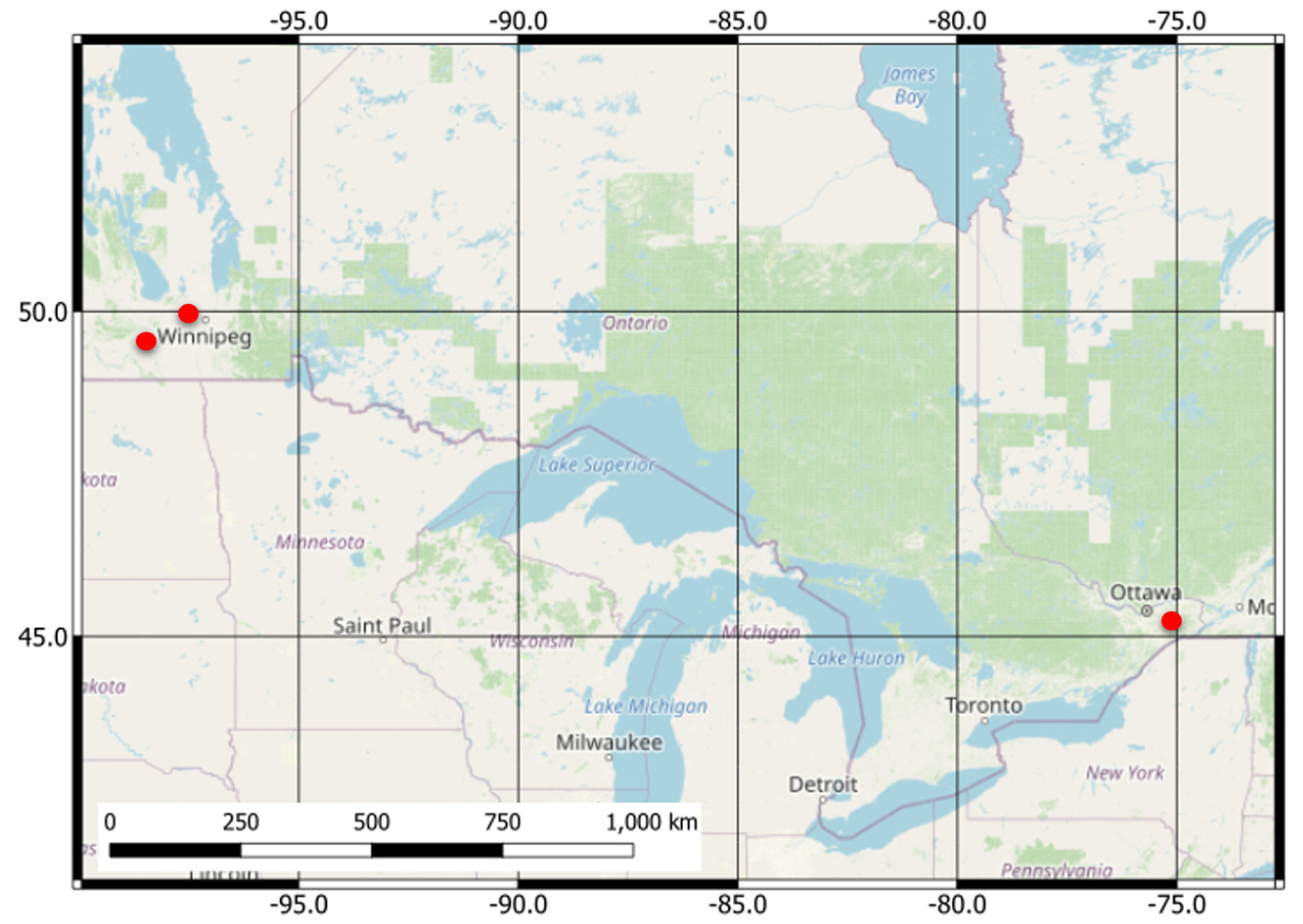
We selected two well-known Canadian experimental sites located in Ontario and Manitoba. Both sites are equipped with Real-Time In Situ Soil Monitoring for Agriculture (RISMA) stations. These stations include Stevens HydraProbe sensors that record the soil temperature and the real part of the dielectric constant, which is converted to a volumetric soil moisture value [21]. The first site is situated within the South Nation River watershed, in close proximity to the town of Casselman, southeast of Ottawa. This site encompasses one RISMA network with four stations (Figure 1).

The second site comprises two RISMA networks located in southern Manitoba. The first network includes nine RISMA stations situated near the towns of Carman and Elm Creek, southwest of Winnipeg. The second network consists of three stations, located immediately northwest of Winnipeg within the Sturgeon Creek watershed (Figure 1). Both the first and second test sites share a common characteristic of intensive agriculture activities, predominantly focusing on annual crops [22].

In our study, we considered the integrated soil moisture from a depth of 0 to 5 cm measured by the RISMA stations. However, during the early spring thaw, we switched to the measured soil moisture at a 5 cm depth instead. The reason for this change is that the 0–5 cm sensor probes, which are inserted vertically into the soil surface, are affected by frost during the thaw, causing them to be partially pushed out of the ground. As a result, the exposed probe tines interact with the air, leading to lower dielectric values. This, in turn, causes an underestimation of the integrated soil moisture measured from a depth of 0 to 5 cm. To address this issue, Agriculture and Agri-Food Canada (AAFC) conducts necessary maintenance of the stations annually by resetting the surface probes that might have been displaced, usually before the middle of May.

The experimental dataset consisted of 31 RCM images acquired using the SC30M Compact Polarimetric (SC30MCP) imaging mode with a 30 m spatial resolution over the two chosen sites. The RCM images were acquired during the spring (15 April–28 June) and fall (15 September–27 October) of 2022. Consequently, the fields were characterized by unvegetated bare soil with a relatively smooth random roughness state. Consequently, the backscattered radar signal should be associated with the real part of the soil’s dielectric constant. Additionally, the weather data gathered by the RISMA stations were utilized to verify the absence of snow and frozen soil conditions during spring and fall.

4. Methodology

4.1. SAR Processing

The acquired RCM images were processed as Multi-Look Complex (MLC) products, providing the backscattered signal amplitude and phase information. To minimize speckle noise, a 3 × 3 boxcar filter was applied to the acquired images. Next, we extracted the 25 CP features described in Section 2. All extracted features were sampled at the location of the RISMA stations. Subsequently, an experimental sample dataset was constructed consisting of 236 samples. Each sample corresponds to the values of the extracted CP features at the location of a RISMA station, as well as the local radar incidence angle and the average recorded soil moisture content at the time of the SAR image acquisition.

The constructed experimental dataset of our study is characterized by a variety of soil moisture conditions, ranging from 4.9% (very dry conditions) to 51.3% (very wet conditions). However, most of the dataset samples had medium soil moisture values in the range of 20–40%. The minimum radar incidence angle in the sample dataset is 21.9°, while the maximum is 41.4°. This is intentional following a recommendation by the RCM’s calibration and validation team, confirming the minor impact of the imperfect emitted RCM circular polarization signal triggered by a dissimilarity between the H and V antenna gains for a radar incidence angle between 20° and 43°. Within this range, the axis ratio of the transmitted signal is <0.5 dB [16].

4.2. Soil Moisture Retrieval Framework

4.2.1. Feature Selection

In this study, we propose a strategy to select the input features with low correlation between each other and higher importance for soil moisture retrieval. This strategy is depicted in the flowchart in Figure 2.

At first, we calculated the absolute value of the Spearman Correlation Coefficient (SCC) for all input CP features. The SCC, a nonparametric correlation coefficient with a range of −1 to 1, reveals the monotonic relationship between variables, enabling us to avoid the need for assumptions about the statistical distribution of the CP features. Next, the Univariate Feature Ranking F-test statistics was applied to examine the importance of the CP features. The Univariate Feature Ranking F-test is a statistical test that compares the null hypothesis that the response values grouped by the predictor variable values are drawn from populations with the same mean against the alternative hypothesis that the population means differ. A test statistic with a small $p$-value indicates that the corresponding predictor is important. An Importance Score (IS) is calculated as $\mathrm{IS}=-log\left(p\right)$. Therefore, a high IS indicates that the associated predictor is significant. In this work, each CP parameter was treated as a predictor for soil moisture by testing whether the variations In soil moisture as a dependent variable were accounted for by the predictor as an independent variable. Figure 3 shows the ranking of the features according to the F-test statistics. To implement the proposed feature selection strategy, we selected a threshold for the absolute SCC to categorize the correlation between each pair of predictors as either strongly correlated or weakly correlated features. Herein, the absolute SCC threshold was set to 0.90. If the absolute SCC between two predictors was ≥0.90, we assumed the two predictors to be strongly correlated [23,24,25]. In this case, we compared their F-test importance score and selected the feature with the highest importance score to be included in the output feature set (OF-Set). On the other hand, if the correlation value was <0.90, we did not perform the IS test, and the feature was added directly to the OF-Set. The feature selection process started with two initial predictors and the radar Incidence Angle (IA) to form the first input feature set, denoted as IF-Set1. In each subsequent step, one additional input feature was incorporated. For instance, in the second step, we introduced IF-Set2, comprising the outcome feature set from the preceding step, OF-Set1, and the currently introduced input feature. This iterative procedure involved conducting correlation tests and, if deemed necessary, applying the F-Test, continuing until all input features had been thoroughly examined. Each OF-Set was used for the training and validation of the GPR and ENL models.

4.2.2. Machine Learning Implementation

In this study, the Gaussian Process Regression (GPR) and the Ensemble Learning Regression (ELR) were utilized for retrieving the soil moisture. The hyperparameters of these ML regressors were fine-tuned using the Bayesian optimization technique. Bayesian optimization determines the hyperparameter values that minimize a loss or objective function [26]. The Mean Squared Error (MSE) between the predicted and actual objective values was used as the loss function in the current study. The Bayesian optimizer uses the expected improvement per second as the acquisition function [27] to determine the next iteration’s hyperparameter set. The set of model hyperparameters that minimized the upper confidence interval of the MSE objective function was deemed the optimal set, and the corresponding model was used to predict the soil moisture. An eight-fold cross-validation scheme was employed to train and evaluate the machine learning models. Consequently, the sample dataset was divided into eight subsets. During each iteration of this scheme, the models were trained using seven of these subsets, while the remaining one was held out for testing. The reported performance of the models represents the average performance metrics computed across the test subsets over the eight iterations of the cross-validation scheme. In the following sections, we provide a concise description of the GPR and ELR used in this study to retrieve soil moisture.

Gaussian Process Regression

The GPR is a supervised nonparametric ML technique based on the formation of Gaussian process-based time series prediction models [28]. The GPR model requires several hyperparameters to be specified. These hyperparameters consist of the fundamental function of the prior mean function of the GPR, the kernel function that models the correlation in the response variable, the kernel scale that determines the initial kernel parameters, and the standard deviation (Sigma) of the sample noise. In our research, the Bayesian optimization method selects the optimal hyperparameters from the ranges shown in

Table 1. The ranges of the GPR optimizable hyperparameters. $X$ is the input predictor, $R$ is the response variable, and $SD$ is the standard deviation.

Optimizable Hyperparameters	Range
Fundamental Function	Zero, Constant, Linear
Kernel Function	Nonisotropic/Isotropic (Rational Quadratic, Squared Exponential, Exponential, Matern 5/2, Matern 3/2)
Kernel Scale	$\left[0.001,1\right] \times max\left(max\left(X\right)-min\left(X\right)\right)$
Sigma	$\left[0.0001,max\left(0.001,10 \times SD\left(R\right)\right)\right]$

. The optimization curve of the best GPR model and its optimal hyperparameters are presented in the next section.

Ensemble Learning Regression

The ELR is an ML approach that employs multiple ML models instead of a single model to resolve nonlinear regression problems [29]. An ensemble of decision-tree-based models (weak learners) is generated and integrated to form a robust prediction model. In our study, we investigated Boosted trees and Bagged trees using Bayesian optimization for the regression problem. In the Boosted trees, the ensemble method is Least Squares Boosting (LSBoost) with Regression Trees (RT) learners. On the contrary, Bootstrap bagging (Bag) with RT learners is the ensemble style of Bagged trees. The minimum leaf size, learning rate, number of learners, and number of predictors to sample are the ensemble models’ optimizable hyperparameters. The ranges of these hyperparameters to be sought by the Bayesian optimization method are presented in

Table 2. The ranges of the ensemble model’s optimizable hyperparameters. $S$ is the number of samples and $P_r$ is the number of input predictors.

Optimizable Hyperparameters	Range
Ensemble Method	Bag, LSBoost
Minimum leaf size	$[1,max\left(2,floor\left(\mathrm{S}/2\right)\right)$
Number of learners	[10, 500]
Learning rate	[0.001, 1]
Number of predictors to sample	$\left[1,max\left(2,P_r\right)\right]$

. The optimization curve of the best ELR model and its optimized hyperparameters are depicted in the next section.

5. Results and Discussion

The feature selection process started with two features which we randomly selected: s3 and mchi_surf. The absolute correlation between s3 and mchi_surf was 0.96, indicating a strong correlation between the two features. we examined the importance scores, finding that the importance score of mchi_surf was higher than that of s3. Consequently, we selected mchi_surf to be included with the IA, forming the first output feature set (OF-Set1), as shown in

Table 3. Performance of the ML soil moisture prediction models trained using a feature set formed through the proposed feature selection approach. Entries of the best performance GPR and ELR are depicted in bold. Feature sets that stayed the same as in their previous steps were not used for training or evaluation the ML models. Therefore, the performance metrics entries are shaded in grey. # indicates the number.

Starting Features: s3, mchi_surf, IA			# F in OF-Set	Optimized Hyperparameters GPR		Optimized Hyperparameters ELR
IF-Set #	Added Feature	Output Feature Set (OF-Set) Composition		R2	RMSE (%)	R2	RMSE (%)
1	The Starting Features	mchi_surf, IA	2	0.62	6.75	0.51	7.67
2	mu	mchi_surf, mu, IA	3	0.72	5.79	0.56	7.22
3	mc	Same as step 2	3
4	delta	mchi_surf, mu, delta, IA	4	0.71	5.87	0.56	7.22
5	SE	mchi_surf, mu, delta, SE, IA	5	0.73	5.67	0.55	7.32
6	alpha	mchi_surf, mu, alpha, SE, IA	6	0.64	6.54	0.41	8.38
7	${\mathsf{\sigma }}_{\mathrm{RL}}^0$	mchi_surf, mu, alpha, ${\mathsf{\sigma }}_{\mathrm{RL}}^0$, IA	5	0.66	6.35	0.49	7.73
8	cp_ratio	Same as step 7	5
9	s2	mchi_surf, mu, alpha, ${\mathsf{\sigma }}_{\mathrm{RL}}^0$, s2, IA	6	0.61	6.80	0.57	7.13
10	SEI	mchi_surf, mu, alpha, ${\mathsf{\sigma }}_{\mathrm{RL}}^0$, s2, SE, IA	7	0.66	6.37	0.58	7.08
11	s0	mchi_surf, mu, alpha, ${\mathsf{\sigma }}_{\mathrm{RL}}^0$, s2, s0, IA	7	0.65	6.45	0.60	6.88
12	mchi_vol	Same as step 11	7
13	ml	mchi_surf, mu, alpha, ${\mathsf{\sigma }}_{\mathrm{RL}}^0$, s2, s0, ml, IA	8	0.67	6.21	0.56	7.18
14	${\mathsf{\sigma }}_{\mathrm{RH}}^0$	mchi_surf, mu, alpha, ${\mathsf{\sigma }}_{\mathrm{RL}}^0$, s2, ${\mathsf{\sigma }}_{\mathrm{RH}}^0$, ml, IA	8	0.60	6.88	0.50	7.74
15	SEP	Same as step 14	8
16	mdelta_vol	Same as step 14	8
17	m	mchi_surf, m, alpha, ${\mathsf{\sigma }}_{\mathrm{RL}}^0$, s2, ${\mathsf{\sigma }}_{\mathrm{RH}}^0$, ml, IA	8	0.60	6.89	0.52	7.60
18	${\mathsf{\sigma }}_{\mathrm{RR}}^0$	mchi_surf, m, alpha, ${\mathsf{\sigma }}_{\mathrm{RL}}^0$, s2, ml, IA	7	0.62	6.70	0.50	7.69
19	s1	mchi_surf, m, alpha, ${\mathsf{\sigma }}_{\mathrm{RL}}^0$, s2, ml, s1, IA	8	0.66	6.35	0.50	7.69
20	mchi_dbl	mchi_surf, m, alpha, ${\mathsf{\sigma }}_{\mathrm{RL}}^0$, s2, ml, s1, mchi_dbl, IA	9	0.69	6.11	0.49	7.80
21	mdelta_dbl	mchi_surf, m, alpha, ${\mathsf{\sigma }}_{\mathrm{RL}}^0$, s2, ml, s1, mdelta_dbl, IA	10	0.64	6.51	0.42	8.32
22	${\mathsf{\sigma }}_{\mathrm{RV}}^0$	Same as step 21	10
23	lp_ratio	mchi_surf, m, alpha, ${\mathsf{\sigma }}_{\mathrm{RL}}^0$, s2, ml, mdelta_dbl, lp_ratio, IA	9	0.68	6.12	0.54	7.38
24	mdelta_surf	Same as step 23

. In the second step, the mu feature was added to the OF-Set1 to form IF-Set2, which consisted of the mu and mchi_surf predictor, in addition to the IA. The SCC between mu and mchi_surf was low, which indicates low dependency between these two features. Therefore, both features were kept in the OF-Set2. In third step, we compared the absolute SCC values of the mc predictor with those of OF-Set2, specifically mu and mchi_surf. The comparison showed a high correlation between the mc and the other two features. Therefore, the IS of mc was assessed in comparison to that of mu and mchi_surf, revealing that mc was of lower importance than both features. Accordingly, mc was discarded, and the OF-Set3 had the same features as the OF-Set2 (Table 3). All the OF-Sets obtained from repeating this procedure for all CP features are presented in Table 3. Moreover, Table 3 shows the estimated RMSE and R² for each model during the training and validation of the GPR and ELR models in an eight-fold cross-validation scheme using each OF-Set. The highest prediction performance was recorded for the optimized GPR classifier when trained with OF-Set5. The RMSE and R² values of this model were 5.67% and 0.73, respectively, and the feature set was composed of mchi_surf, mu, delta, SE, and IA. The optimal hyperparameters of this model had a Zero fundamental function, a Nonisotropic Exponential kernel function, and a Sigma value of $107.69$. These hyperparameters were selected at the observed minimum MSE value of 32.14.

On the other hand, the optimized ELR model achieved its best performance when it was trained with the OF-Set11, including the features: mchi_surf, mu, alpha, ${\mathsf{\sigma }}_{\mathrm{RL}}^0$, s2, s0, and IA. This prediction model recorded RMSE = 6.88% and R² = 0.60. The hyperparameter optimization of this model was obtained at an observed minimum MSE value of 49.3892. The optimal model emerged as an LSBoost ensemble, configured with a minimum leaf size of 1 and a total of 500 learners. The model learning rate was equal to 0.047032 and the predictor-to-sample ratio was equal to 3.

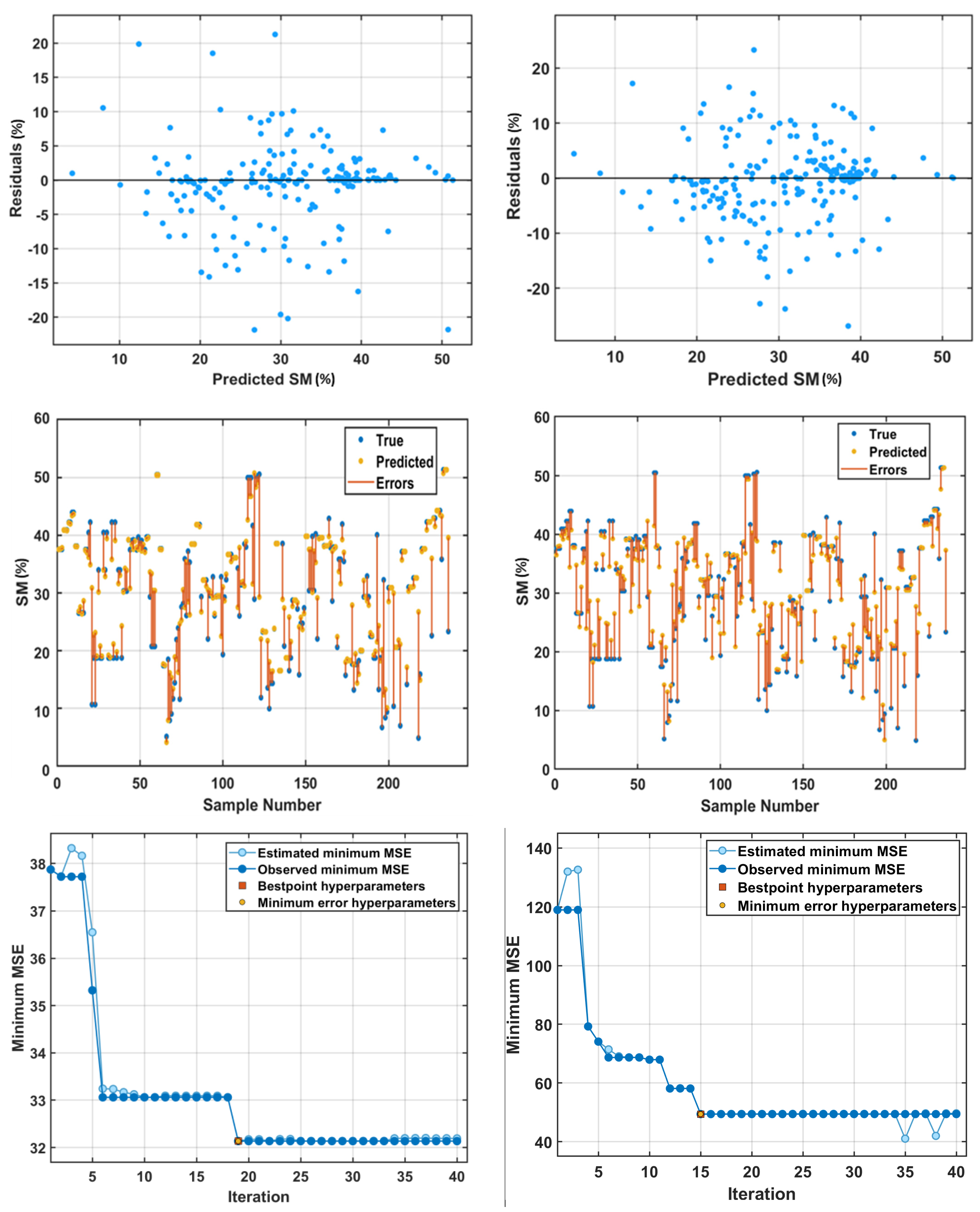
Figure 4 presents the scatter plots, residual plots, and response plots with error bars for the top-performing GPR and ELR models. Additionally, it shows the minimum MSE plots across 30 iterations of the Bayesian-based hyperparameter optimization process. The scatter plots reveal the goodness-of-fit between the true response variable values and the ML prediction models. It is noticeable that a greater number of predicted soil moisture values from the GPR model align with the diagonal perfect-fit line, compared to those predicted by the ELR model. This is consistent with the ${\mathrm{R}}^2$ values of their corresponding models, as depicted in Table 3 (0.73 for the best GPR model against 0.60 for the best ELR model). The residual plots present the difference between the true and predicted soil moisture values for the input samples (Figure 4). The residual plot of the GPR model shows a random pattern with an error range of ±15% about the horizontal line at 0, with few outliers. This is also the case for the ELR residual plot (Figure 4). The scatter plots along with the residual plots give insight into the correlation between the true soil moisture values and the values predicted by both models. This is further indicated in the response plots in Figure 4, which show the true and predicted response values for the data samples. The error bars in the response plots show the difference between the true and predicted values generated by the corresponding ML models. The ELR model achieves a correlation R between true and predicted soil moisture values equal to 0.75, while the GPR achieves a correlation equal to 0.85. From the minimum MSE plots of the ML models, we can see that the optimum ELR hyperparameters recorded an observed minimum MSE of 49.4 at the 15th iteration, while the GPR optimal hyperparameters were recorded at the 19th iteration, and its corresponding observed minimum MSE value was 32.13.

6. Conclusions

In this study, we investigated the potential of the RCM CP mode for soil moisture retrieval over bare soil. A dataset comprising 25 CP features along with the radar incidence angles sampled from acquired RCM images at the location of RISMA stations in ON and MB was used. A framework was developed for the optimal selection of CP features. Through the implementation of the proposed feature selection framework, subsets of CP features were extracted, consisting of less correlated CP features significant for soil moisture retrieval. Two ML models were examined for the soil moisture retrieval: GPR and ELR. The Bayesian optimization strategy was employed for fine-tuning the hyperparameters of both models. The results of our study reveal the encouraging performance of the optimized GPR model for soil moisture retrieval using four CP features: mchi_surf, mu, delta, and SE. The GPR model recorded an RMSE value of 5.67% and R² value of 0.73. The optimized ELR model achieved its highest performance with a combination of six CP features: mchi_surf, mu, alpha, ${\mathsf{\sigma }}_{\mathrm{RL}}^0$, s2, and s0, resulting in RMSE = 6.88% and R² = 0.60. Both models included the radar IA with the CP features. The findings of our study emphasize the potential for soil moisture retrieval through the utilization of the RCM SC30MCP mode in conjunction with ML techniques.

References

- Chung, J.; Lee, Y.; Kim, J.; Jung, C.; Kim, S. Soil moisture content estimation based on Sentinel-1 SAR imagery using an artificial neural network and hydrological components. Remote Sens. 2022, 14, 465. [Google Scholar] [CrossRef]
- Seung-Bum, K.; Tien-Hao, L. Robust retrieval of soil moisture at field scale across wide-ranging SAR incidence angles for soybean, wheat, forage, oat and grass. Remote Sens. Environ. 2021, 266, 112712. [Google Scholar]
- Dabboor, M.; Sun, L.; Carrera, M.L.; Friesen, M.; Merzouki, A.; McNairn, H.; Powers, J.; Bélair, S. Comparative analysis of high-resolution soil moisture simulations from the soil, vegetation, and Snow (SVS) land surface model using SAR imagery over bare soil. Water 2019, 11, 542. [Google Scholar] [CrossRef]
- Merzouki, A.; McNairn, H. A hybrid (multi-angle and multipolarization) approach to soil moisture retrieval using the integral equation model: Preparing for the RADARSAT constellation mission. Can. J. Remote Sens. 2015, 41, 349–362. [Google Scholar] [CrossRef]
- Séguin, G.; Ahmed, S. RADARSAT constellation, project objectives and status. In Proceedings of the IEEE International Geoscience and Remote Sensing Symposium, Cape Town, South Africa, 12–17 July 2009; pp. II–894–II-897. [Google Scholar]
- Dabboor, M.; Olthof, I.; Mahdianpari, M.; Mohammadimanesh, F.; Shokr, M.; Brisco, B.; Homayouni, S. The RADARSAT Constellation Mission Core Applications: First Results. Remote Sens. 2022, 14, 301. [Google Scholar] [CrossRef]
- Raney, R.K. Hybrid-polarity SAR architecture. IEEE Trans. Geosci. Remote Sens. 2007, 45, 3397–3404. [Google Scholar] [CrossRef]
- Williams, M.L. Potential for surface parameter estimation using compact polarimetric SAR. IEEE Geosci. Remote Sens. Lett. 2009, 5, 471–473. [Google Scholar] [CrossRef]
- Truong-Loï, M.; Freeman, A.; Dubois-Fernandez, P.; Pottier, E. Estimation of soil moisture and Faraday rotation from bare surfaces using compact polarimetry. IEEE Trans. Geosci. Remote Sens. 2009, 47, 3608–3615. [Google Scholar] [CrossRef]
- Charbonneau, F.; Brisco, B.; Raney, K.; McNairn, H.; Liu, C.; Vachon, P.; Shang, J.; De Abreu, R.; Champagne, C.; Merzouki, A.; et al. Compact polarimetry overview and applications assessment. Can. J. Remote Sens. 2010, 36, S298–S315. [Google Scholar] [CrossRef]
- Ouellette, J.D.; Johnson, J.T.; Kim, S.; Van Zyl, J.; Moghaddam, M.; Spencer, M.W.; Tsang, L.; Entekhabi, D. A simulation study of compact polarimetry for radar retrieval of soil moisture. IEEE Trans. Geosci. Remote Sens. 2014, 52, 5966–5973. [Google Scholar] [CrossRef]
- Das, K.; Paul, P. Soil moisture retrieval model by using RISAT-1, C-band data in tropical dry and sub-humid zone of Bankura district of India. Egypt. J. Remote Sens. Space Sci. 2015, 18, 297–310. [Google Scholar] [CrossRef]
- Ponnurangam, G.G.; Jagdhuber, T.; Hajnsek, I.; Rao, Y.S. Soil moisture estimation using hybrid polarimetric SAR data of RISAT-1. IEEE Trans. Geosci. Remote Sens. 2016, 54, 2033–2049. [Google Scholar] [CrossRef]
- Merzouki, A.; McNairn, H.; Powers, J.; Friesen, M. Synthetic aperture radar (SAR) compact polarimetry for soil moisture retrieval. Remote Sens. 2019, 11, 2227. [Google Scholar] [CrossRef]
- Santi, E.; Dabboor, M.; Pettinato, S.; Paloscia, S. Combining machine learning and compact polarimetry for estimating soil moisture from C-band SAR data. Remote Sens. 2019, 11, 2451. [Google Scholar] [CrossRef]
- Dabboor, M.; Atteia, G.; Meshoul, S.; Alayed, W. Deep Learning-Based Framework for Soil Moisture Content Retrieval of Bare Soil from Satellite Data. Remote Sens. 2023, 15, 1916. [Google Scholar] [CrossRef]
- Raney, R.K.; Spudis, P.D.; Bussey, B.; Crusan, J.; Jensen, J.R.; Marinelli, W.; Neish, C.; Palsetia, M.; Schulze, R.; Sequeira, H.B.; et al. The lunar mini-RF radars: Hybrid polarimetric architecture and initial results. Proc. IEEE 2011, 99, 808–823. [Google Scholar] [CrossRef]
- Raney, R.K. Dual-polarized SAR and Stokes parameters. IEEE Geosci. Remote Sens. Lett. 2006, 3, 317–319. [Google Scholar] [CrossRef]
- Cloude, S.R.; Goodenough, D.G.; Chen, H. Compact decomposition theory. IEEE Trans. Geosci. Remote Sens. 2011, 9, 28–32. [Google Scholar] [CrossRef]
- Réfrégier, P.; Morio, J. Shannon entropy of partially polarized and partially coherent light with Gaussian fluctuations. J. Opt. Soc. Am. A 2006, 23, 3036–3044. [Google Scholar] [CrossRef]
- Pacheco, A.; L’Heureux, J.; McNairn, H.; Powers, J.; Howard, A.; Geng, X.; Rollin, P.; Gottfried, K.; Freeman, J.; Ojo, R.; et al. Real-Time In-Situ Soil Monitoring for Agriculture (RISMA) Network Metadata; Agriculture and Agri-Food Canada: Edmonton, AB, Canada. Available online: https://agriculture.canada.ca/SoilMonitoringStations/files/RISMA_Network_Metadata.pdf (accessed on 5 April 2022).
- McNairn, H.; Jackson, T.J.; Wiseman, G.; Belair, S.; Berg, A.; Bullock, A.; Colliander, A.; Cosh, M.H.; Kim, S.B.; Magagi, R.; et al. The soil moisture active passive validation experiment 2012 (SMAPVEX12): Prelaunch calibration and validation of the SMAP soil moisture algorithms. IEEE Trans. Geosci. Remote Sens. 2015, 53, 2784–2801. [Google Scholar] [CrossRef]
- Desbordes, P.; Ruan, S.; Modzelewski, R.; Pineau, P.; Vauclin, S.; Gouel, P.; Michel, P.; Di Fiore, F.; Vera, P.; Gardin, I. Predictive value of initial FDG-PET features for treatment response and survival in esophageal cancer patients treated with chemo-radiation therapy using a random forest classifier. PLoS ONE 2017, 12, e0173208. [Google Scholar] [CrossRef] [PubMed]
- Dabboor, M.; Montpetit, B.; Howell, S.; Haas, C. Improving sea ice characterization in dry ice winter conditions using polarimetric parameters from C- and L-band SAR data. Remote Sens. 2017, 9, 1270. [Google Scholar] [CrossRef]
- Dabboor, M.; Montpetit, B.; Howell, S. Assessment of the high resolution SAR mode of the RADARSAT constellation mission for first year ice and multiyear ice characterization. Remote Sens. 2018, 10, 594. [Google Scholar] [CrossRef]
- Astudillo, R.; Frazier, P.I. Bayesian Optimization of Function Networks. In Proceedings of the 35th Conference on Neural Information Processing Systems, Online, 6–14 December 2021. [Google Scholar]
- Rasmussen, C.E.; Williams, C.K.I. Gaussian Processes for Machine Learning; The MIT Press: Cambridge, MA, USA, 2005. [Google Scholar]
- Stamenkovic, J.; Guerriero, L.; Ferrazzoli, P.; Notarnicola, C.; Greifeneder, F.; Thiran, J.P. Soil moisture estimation by SAR in alpine fields using gaussian process regressor trained by model simulations. IEEE Trans. Geosci. Remote Sens. 2017, 55, 4899–4912. [Google Scholar] [CrossRef]
- Shirmard, H.; Farahbakhsh, E.; Müller, R.D.; Chandra, R. A review of machine learning in processing remote sensing data for mineral exploration. Remote Sens. Environ. 2022, 268, 112750. [Google Scholar] [CrossRef]