
Evaluating Spatial-Temporal Clogging Evolution in a Meso-Scale Lysimeter

Abstract
:1. Introduction
2. Materials and Methods
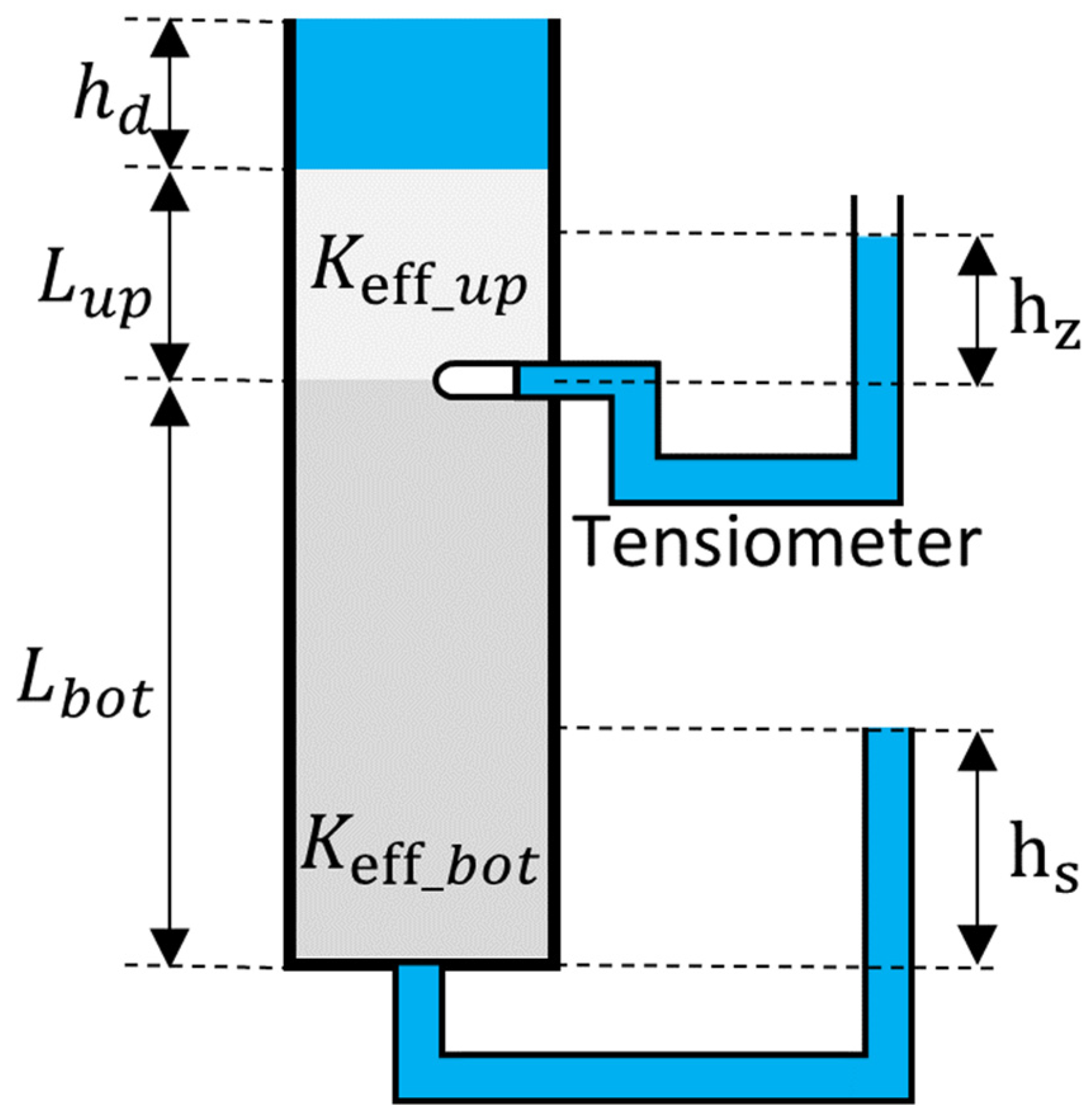
2.1. - Diagram
2.2. Case Study with Lysimeter Experiments
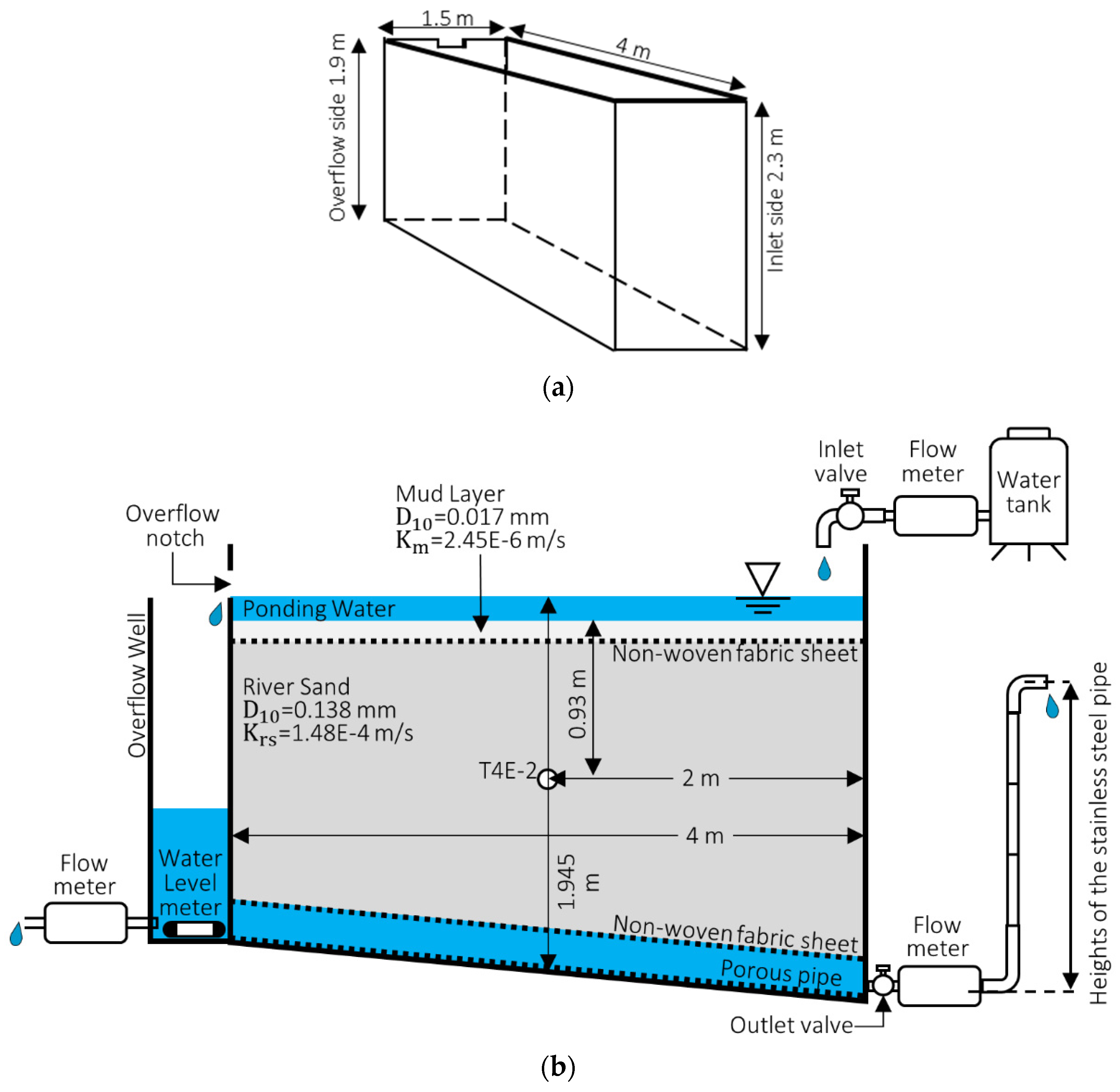
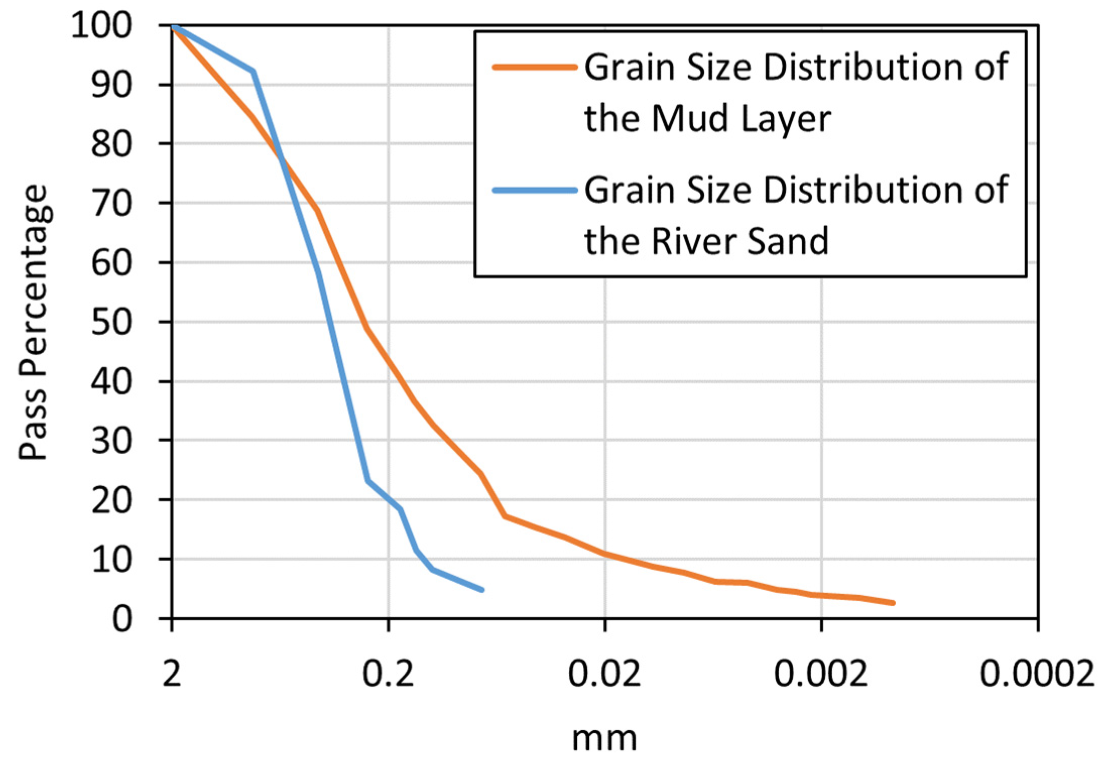
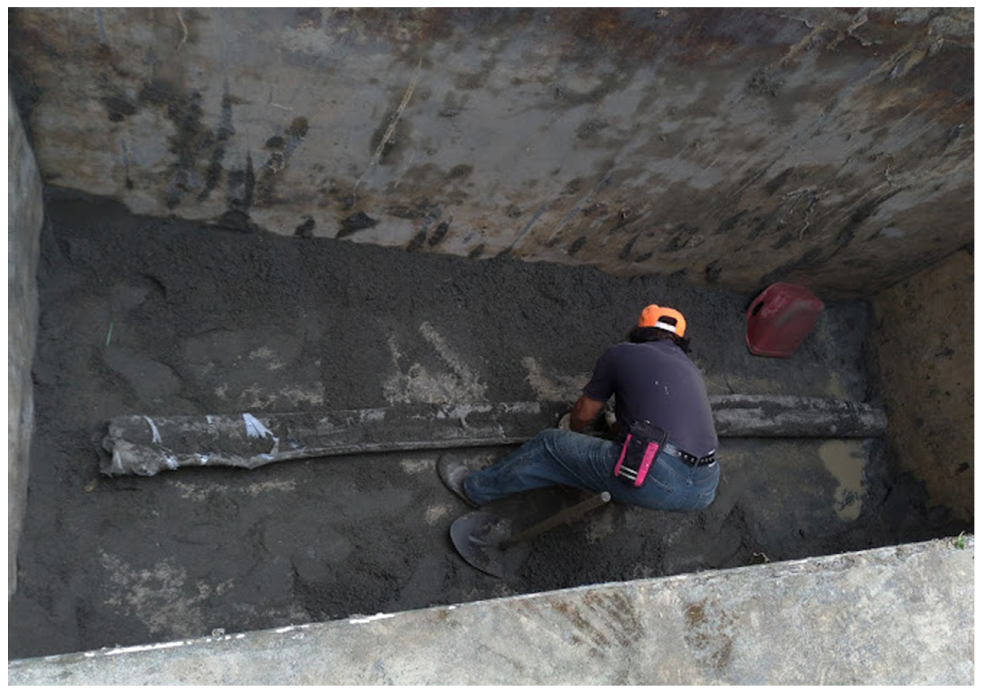
2.2.1. Setup of Lysimeter Experiments
2.2.2. Process of Infiltration Experiments with the Lysimeter
2.3. The Lysimeter Simulation
3. Results
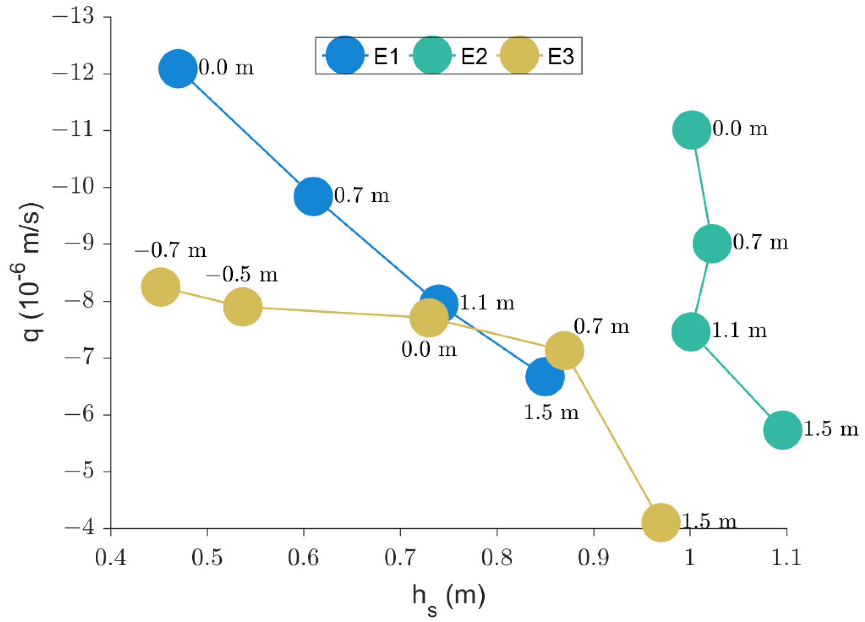
3.1. Measured Data in the Lysimeter and
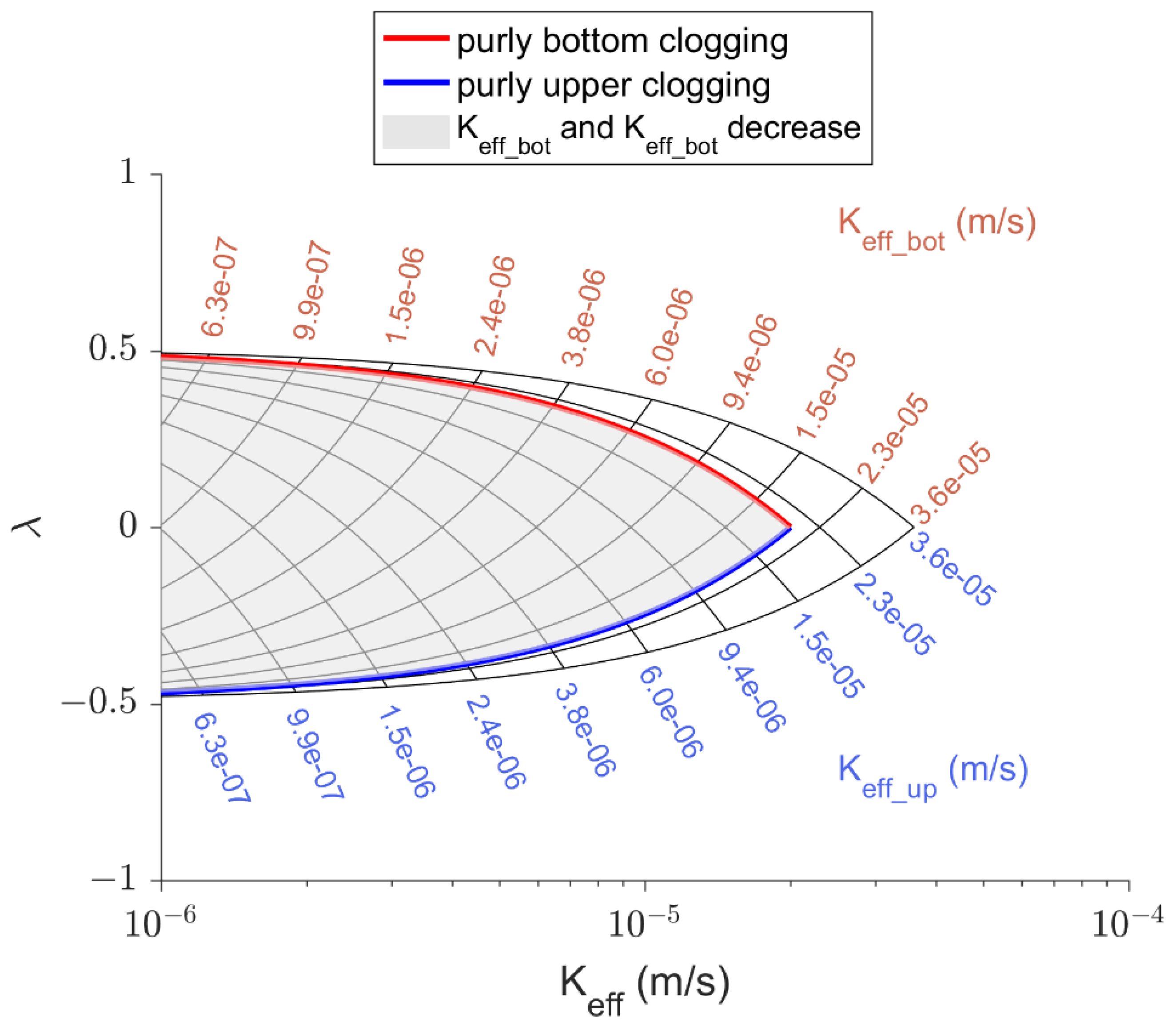
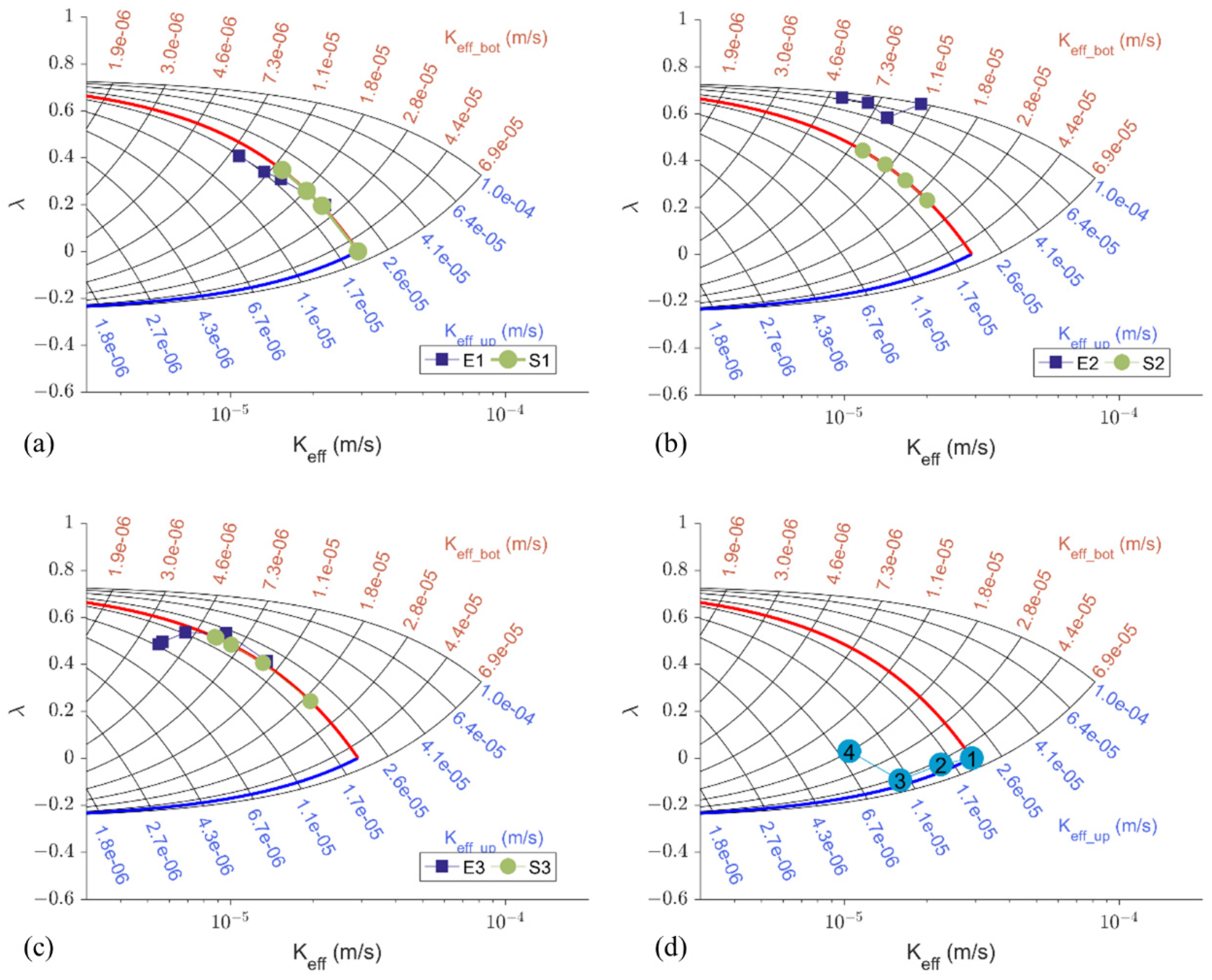
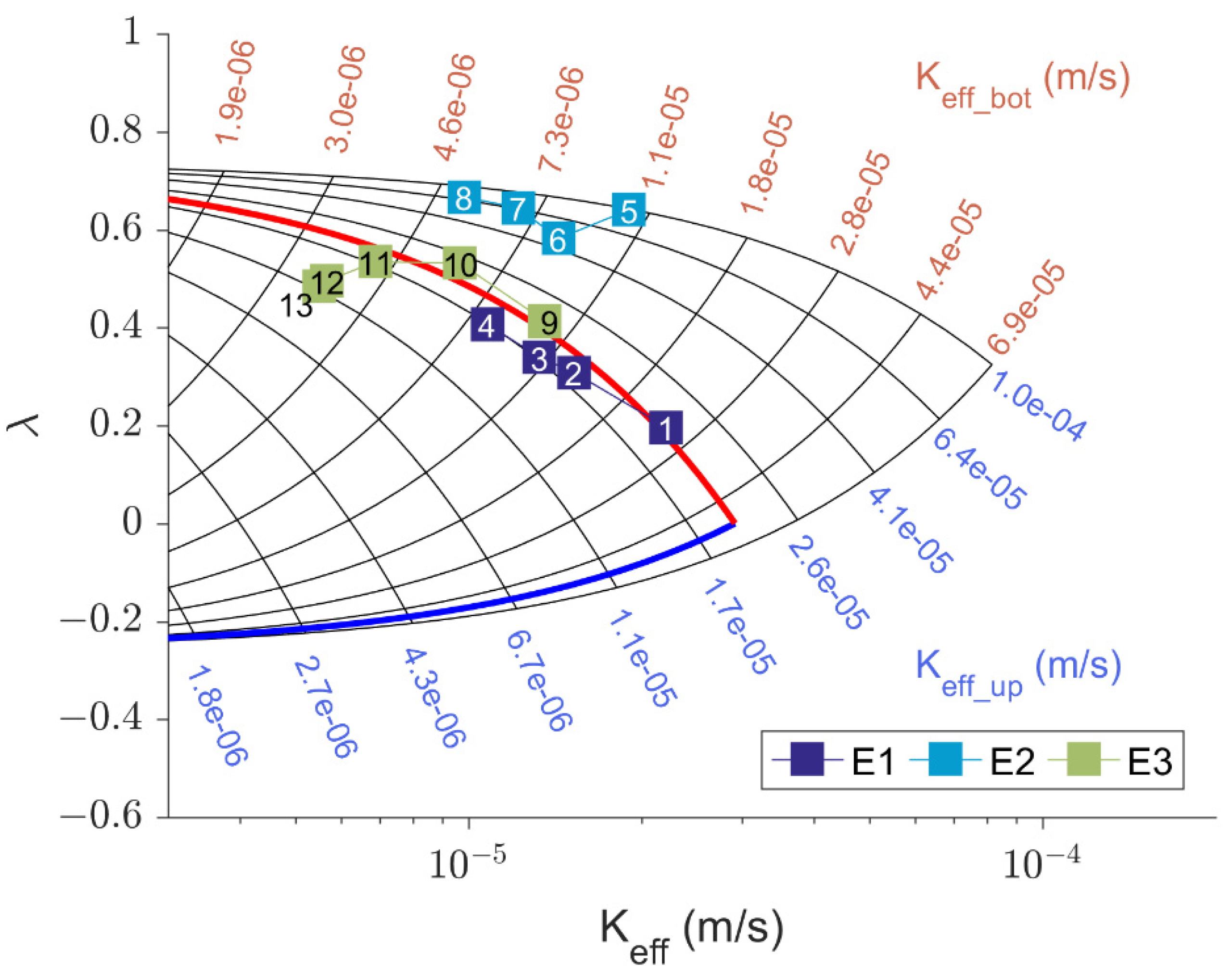
3.2. Experimental Data in the - Diagram and Diagram Validation
4. Discussions
4.1. and from Experiments and Simulation
4.2. Increasing and Reducing in Each Experimental Cycle
4.3. Recovery of When Performing the Next Cycle
4.4. Unsaturated Zone Development
5. Conclusions
Author Contributions
Funding
Institutional Review Board Statement
Informed Consent Statement
Data Availability Statement
Acknowledgments
Conflicts of Interest
References
- Rogers, D.B.; Newcomer, M.E.; Raberg, J.H.; Dwivedi, D.; Steefel, C.; Bouskill, N.; Nico, P.; Faybishenko, B.; Fox, P.; Conrad, M.; et al. Modeling the Impact of Riparian Hollows on River Corridor Nitrogen Exports. Front. Water 2021, 3, 248–265. [Google Scholar] [CrossRef]
- Blaschke, A.P.; Steiner, K.H.; Schmalfuss, R.; Gutknecht, D.; Sengschmitt, D. Clogging processes in hyporheic interstices of an impounded river, the Danube at Vienna, Austria. Int. Rev. Hydrobiol. A J. Cover. All Asp. Limnol. Mar. Biol. 2003, 88, 397–413. [Google Scholar] [CrossRef]
- Chiu, Y.-C.; Lee, T.-Y.; Hsu, S.-Y.; Liao, L.-Y. The effect of hydrological conditions and bioactivities on the spatial and temporal variations of streambed hydraulic characteristics at the subtropical alpine catchment. J. Hydrol. 2020, 584, 124665. [Google Scholar] [CrossRef]
- Joppen, M.; Sulser, P.; Blaser, P.; Kohler, A. Einfluß der Stauregelung auf Grundwasser. Wasserbau München–Obernach Mitt. 1992, 29, 365–375. [Google Scholar]
- Lisle, T.E. Sediment transport and resulting deposition in spawning gravels, north coastal California. Water Resour. Res. 1989, 25, 1303–1319. [Google Scholar] [CrossRef]
- Newcomer, M.E.; Hubbard, S.S.; Fleckenstein, J.H.; Maier, U.; Schmidt, C.; Thullner, M.; Ulrich, C.; Flipo, N.; Rubin, Y. Simulating bioclogging effects on dynamic riverbed permeability and infiltration. Water Resour. Res. 2016, 52, 2883–2900. [Google Scholar] [CrossRef]
- Ulrich, C.; Hubbard, S.S.; Florsheim, J.; Rosenberry, D.; Borglin, S.; Trotta, M.; Seymour, D. Riverbed Clogging Associated with a California Riverbank Filtration System: An Assessment of Mechanisms and Monitoring Approaches. J. Hydrol. 2015, 529, 1740–1753. [Google Scholar] [CrossRef]
- Brunner, P.; Cook, P.G.; Simmons, C.T. Hydrogeologic controls on disconnection between surface water and groundwater. Water Resour. Res. 2009, 45. [Google Scholar] [CrossRef]
- Osman, Y.Z.; Bruen, M.P. Modelling stream-aquifer seepage in an alluvial aquifer: An improved loosing-stream package for MODFLOW. J. Hydrol. 2002, 264, 69–86. [Google Scholar] [CrossRef]
- Fox, G.A.; Durnford, D.S. Unsaturated hyporheic zone flow in stream/aquifer conjunctive systems. Adv. Water Resour. 2003, 26, 989–1000. [Google Scholar] [CrossRef]
- Winter, T.C.; Harvey, J.W.; Franke, O.L.; Alley, W.M. Ground Water and Surface Water: A Single Resource, Circular 1139; US Geological Survey: Denver, CO, USA, 1998; p. 79. [Google Scholar]
- Rivière, A.; Goncalves, J.; Jost, A.; Font, M. Experimental and numerical assessment of transient stream–aquifer exchange during disconnection. J. Hydrol. 2014, 517, 574–583. [Google Scholar] [CrossRef] [Green Version]
- Jha, M.K.; Mahapatra, S.; Mohan, C.; Pohshna, C. Infiltration characteristics of lateritic vadose zones: Field experiments and modeling. Soil Tillage Res. 2019, 187, 219–234. [Google Scholar] [CrossRef]
- Liu, C.-W.; Chen, S.-K.; Jang, C.-S. Modelling water infiltration in cracked paddy field soil. Hydrol. Processes 2004, 18, 2503–2513. [Google Scholar] [CrossRef]
- Hsieh, C.-H.; Davis, A.P. Evaluation and Optimization of Bioretention Media for Treatment of Urban Storm Water Runoff. J. Environ. Eng. 2005, 131, 1521–1531. [Google Scholar] [CrossRef]
- Li, H.; Davis, A.P. Urban Particle Capture in Bioretention Media. I: Laboratory and Field Studies. J. Environ. Eng. 2008, 134, 409–418. [Google Scholar] [CrossRef]
- Hatt, B.E.; Siriwardene, N.; Deletic, A.; Fletcher, T.D. Filter media for stormwater treatment and recycling: The influence of hydraulic properties of flow on pollutant removal. Water Sci. Technol. 2006, 54, 263–271. [Google Scholar] [CrossRef]
- Glover, P.W.; Walker, E. Grain-size to effective pore-size transformation derived from electrokinetic theory. Geophysics 2009, 74, E17–E29. [Google Scholar] [CrossRef]
- Kale, R.V.; Sahoo, B. Green-Ampt infiltration models for varied field conditions: A revisit. Water Resour. Manag. 2011, 25, 3505–3536. [Google Scholar] [CrossRef]
- Ranjbaran, M.; Datta, A.K. Retention and infiltration of bacteria on a plant leaf driven by surface water evaporation. Phys. Fluids 2019, 31, 112106. [Google Scholar] [CrossRef]
- Biot, M.A. General theory of three-dimensional consolidation. J. Appl. Phys. 1941, 12, 155–164. [Google Scholar] [CrossRef]
- Biot, M.A. Theory of elasticity and consolidation for a porous anisotropic solid. J. Appl. Phys. 1955, 26, 182–185. [Google Scholar] [CrossRef]
- Terzaghi, K. Erdbaumechanik auf Bodenphysikalischer Grundlage; F. Deuticke: Vienna, Austria, 1925. [Google Scholar]


| Experimental Cycle | Sequence No. | Heights of the Stainless-Steel Pipe at the Outlet | The Pore Water Pressure Head from the Tensiometer | Infiltration Flux (m/s) |
|---|---|---|---|---|
| E1 | 1 | 1.5 | 0.850 | −6.67 × 10⁻⁶ |
| 2 | 1.1 | 0.740 | −7.95 × 10⁻⁶ | |
| 3 | 0.7 | 0.610 | −9.84 × 10⁻⁶ | |
| 4 | 0.0 | 0.470 | −1.21 × 10⁻⁵ | |
| E2 | 5 | 1.5 | 1.096 | −5.73 × 10⁻⁶ |
| 6 | 1.1 | 1.001 | −7.46 × 10⁻⁶ | |
| 7 | 0.7 | 1.023 | −9.01 × 10⁻⁶ | |
| 8 | 0.0 | 1.002 | −1.10 × 10⁻⁵ | |
| E3 | 9 | 1.5 | 0.970 | −4.10 × 10⁻⁶ |
| 10 | 0.7 | 0.870 | −7.13 × 10⁻⁶ | |
| 11 | 0.0 | 0.730 | −7.70 × 10⁻⁶ | |
| 12 | −0.5 | 0.537 | −7.90 × 10⁻⁶ | |
| 13 | −0.7 | 0.452 | −8.25 × 10⁻⁶ |
| Scenarios | COMSOL Module | (m) | (m/s) | (m/s) | (m/s) | (m) | (m/s) |
|---|---|---|---|---|---|---|---|
| S1 | Darcy | 1.5 | 2.45 × 10⁻⁶ | 1.48 × 10⁻⁴ | 6.40 × 10⁻⁷ | 0.74 | −8.79 × 10⁻⁶ |
| 1.1 | 2.45 × 10⁻⁶ | 1.48 × 10⁻⁴ | 3.27 × 10⁻⁷ | 0.63 | −1.12 × 10⁻⁵ | ||
| 0.7 | 2.45 × 10⁻⁶ | 1.48 × 10⁻⁴ | 2.66 × 10⁻⁷ | 0.50 | −1.40 × 10⁻⁵ | ||
| 0.0 | 2.45 × 10⁻⁶ | 1.48 × 10⁻⁴ | 1.89 × 10⁻⁷ | 0.35 | −1.73 × 10⁻⁵ | ||
| S2 | Darcy | 1.5 | 2.45 × 10⁻⁶ | 1.48 × 10⁻⁴ | 2.51 × 10⁻⁷ | 0.87 | −6.05 × 10⁻⁶ |
| 1.1 | 2.45 × 10⁻⁶ | 1.48 × 10⁻⁴ | 2.00 × 10⁻⁷ | 0.75 | −8.69 × 10⁻⁶ | ||
| 0.7 | 2.45 × 10⁻⁶ | 1.48 × 10⁻⁴ | 1.57 × 10⁻⁷ | 0.67 | −1.04 × 10⁻⁵ | ||
| 0.0 | 2.45 × 10⁻⁶ | 1.48 × 10⁻⁴ | 1.22 × 10⁻⁷ | 0.54 | −1.31 × 10⁻⁵ | ||
| S3 | Darcy | 1.5 | 2.45 × 10⁻⁶ | 1.48 × 10⁻⁴ | 2.40 × 10⁻⁷ | 0.88 | −5.90 × 10⁻⁶ |
| 0.7 | 2.45 × 10⁻⁶ | 1.48 × 10⁻⁴ | 1.41 × 10⁻⁷ | 0.70 | −9.71 × 10⁻⁶ | ||
| 0.0 | 2.45 × 10⁻⁶ | 1.48 × 10⁻⁴ | 9.89 × 10⁻⁸ | 0.63 | −1.13 × 10⁻⁵ | ||
| −0.5 | 2.45 × 10⁻⁶ | 1.48 × 10⁻⁴ | 8.49 × 10⁻⁸ | 0.57 | −1.24 × 10⁻⁵ | ||
| −0.7 | 2.45 × 10⁻⁶ | 1.48 × 10⁻⁴ | 8.37 × 10⁻⁸ | 0.54 | −1.32 × 10⁻⁵ | ||
| S4 | Richards | 1.5 | 2.45 × 10⁻⁶ | 1.48 × 10⁻⁴ | 6.40 × 10⁻⁷ | 0.74 | −8.79 × 10⁻⁶ |
| 1.1 | 2.45 × 10⁻⁶ | 1.48 × 10⁻⁴ | 6.40 × 10⁻⁷ | 0.42 | −1.17 × 10⁻⁵ | ||
| 0.7 | 2.45 × 10⁻⁶ | 1.48 × 10⁻⁴ | 6.40 × 10⁻⁷ | 0.02 | −1.18 × 10⁻⁵ | ||
| 0.0 | 2.45 × 10⁻⁶ | 1.48 × 10⁻⁴ | 6.40 × 10⁻⁷ | −0.31 | −1.17 × 10⁻⁵ |
Publisher’s Note: MDPI stays neutral with regard to jurisdictional claims in published maps and institutional affiliations. |
© 2022 by the authors. Licensee MDPI, Basel, Switzerland. This article is an open access article distributed under the terms and conditions of the Creative Commons Attribution (CC BY) license (https://creativecommons.org/licenses/by/4.0/).
Share and Cite
Lo, J.-H.; Huang, Q.-Z.; Hsu, S.-Y.; Tsai, Y.-Z.; Lin, H.-Y. Evaluating Spatial-Temporal Clogging Evolution in a Meso-Scale Lysimeter. Land 2022, 11, 1518. https://doi.org/10.3390/land11091518
Lo J-H, Huang Q-Z, Hsu S-Y, Tsai Y-Z, Lin H-Y. Evaluating Spatial-Temporal Clogging Evolution in a Meso-Scale Lysimeter. Land. 2022; 11(9):1518. https://doi.org/10.3390/land11091518
Chicago/Turabian StyleLo, Jui-Hsiang, Qun-Zhan Huang, Shao-Yiu Hsu, Yi-Zhih Tsai, and Hong-Yen Lin. 2022. "Evaluating Spatial-Temporal Clogging Evolution in a Meso-Scale Lysimeter" Land 11, no. 9: 1518. https://doi.org/10.3390/land11091518