Communication

Evaluation of Accuracy Enhancement in European-Wide Crop Type Mapping by Combining Optical and Microwave Time Series

Institute of Geomatics, University of Natural Resources and Life Sciences (BOKU), Peter-Jordan-Straße 82, 1190 Vienna, Austria
*
Author to whom correspondence should be addressed.
Land 2022, 11(9), 1397; https://doi.org/10.3390/land11091397
Submission received: 12 July 2022 / Revised: 18 August 2022 / Accepted: 20 August 2022 / Published: 25 August 2022

Abstract

:
This investigation evaluates the potential of combining Copernicus Sentinel-1 (S1) and Sentinel-2 (S2) satellite data in producing a detailed Land Use and Land Cover (LULC) map with 19 crop type classes and 2 broader categories containing Woodland/Shrubland and Grassland over 28 Member States of Europe (EU-28). The Eurostat Land Use and Coverage Area Frame Survey (LUCAS) 2018 dataset is employed as ground truth for model training and validation. Monthly and yearly optical features from S2 spectral reflectance and spectral indices, alongside decadal (10-days) composites from an S1 microwave sensor, are extracted for the EU-28 territory for 2018 using Google Earth Engine (GEE). Five different feature sets using a mixture of indicators were created as input training data. A Random Forest (RF) machine learning algorithm was applied to classify these feature sets, and the generated classification models were compared using an identical validation dataset. Results show that S1 and S2 yearly features together are able to provide a full coverage map less dependent on cloud effects and having appropriate overall accuracy (OA). Based on this feature set, the 21 classes could be classified with an OA of 78.3% using the independent validation data set. The OA increases to 82.7% by grouping 21 classes into 8 broader categories. The comparison with similar studies using individual S1 and S2 data indicates that combining S1 and S2 time series can attain slightly better results while enhancing spatial coverage.

1. Introduction

Land Use and Land Cover (LULC) maps are used for modeling and monitoring the land surface, for example, studying the carbon cycle, the energy balance, and parameters related to soil health and water conditions [1,2,3].
The European Union (EU) is the greatest worldwide exporter of agri-food products, and 42% of the EU’s area is agricultural farmlands [4,5]. Updated and accurate LULC maps are crucial for change detection analysis and provide necessary baseline information for agriculture and food security [6,7,8]. Independent and timely updated data are required for yield forecasts and to support decisions regarding agricultural crop markets in the EU [9]. LULC maps focused on croplands are significant for monitoring crop type and productivity, crop watering methods as well as crop water productivity [10]. In the future, these maps will also be extremely relevant for monitoring the application and impact of policies such as the European Green Deal.
Earth observation (EO) is well suited for regular LULC mapping [2,8,11] due to the spatial coverage, temporal continuity, and low cost of deployment [3]. The free availability of vast amounts of remote sensing data offers exceptional opportunities to render LULC maps over large areas [12,13]. In this context, Copernicus Sentinel-2 (S2) high-resolution data have become an essential tool for LULC surveying especially concentrated on agricultural activities [14,15]. Worldwide agricultural maps could be generated and provide helpful information to policymakers and farmers [16]. Some examples of application of S2 in agriculture are crop type mapping, crop production and irrigation monitoring, as well as nitrogen content and crop health assessments [15].
The availability of ground truth data for training and assessing the LULC maps is still limited. In this context, a number of studies demonstrated the use of the European Land Use and Cover Area frame Survey (LUCAS) data [17] as training data for LULC mapping. LUCAS is a regular in situ survey performed every three years to collect land cover data over a grid of point locations in the EU.
The LUCAS data was already utilized in some studies. Close et al. [18] used LUCAS 2015 survey and S2 data to classify a region in Belgium. Pflugmacher et al. [19] generated a pan-European land cover map with 13 classes employing LUCAS 2015 survey and Landsat-8 data. Weigand et al. [20] produced a seven-classed land cover map in Germany by using LUCAS 2015 survey and S2 data. Venter et al. [21] created a land cover map of Europe with 8 categories by fusion of Sentinel-1 (S1) and S2 data, utilizing LUCAS 2018 data.
In 2018, the LUCAS collection strategy was further improved with the so-called “Copernicus module” that includes field observations more easily comparable to the spatial sampling of EO image data [17]. Using these data, in combination with S1 image data, d’Andrimont et al. [22] produced a 10 m crop type map of the 28 Member States of Europe (EU-28). The study classified 19 specific crop type classes alongside 2 broad Woodland and Shrubland and Grassland classes using the random forest (RF) algorithm, achieving an overall accuracy (OA) of 74.0%. Ghassemi et al. [23] extended this work to S2 data achieving an OA of 77.6%. However, the efficiency of combining the S1 and S2 time series to produce a LULC map in the mentioned scheme (19 crop types and 2 broad classes) has not yet been assessed.
Progress in the quality and availability of EO data was matched over the past decades by similar performance gains in (cloud) computing. This has also enabled progress in producing land cover and land cover change maps [24]. Google Earth Engine (GEE), for example, is a cloud-based platform that is able to process a high amount of geospatial data [25], such as S1, S2, Landsat-8, Landsat-9, and MODIS. The data and many algorithms such as cloud masking, time-series modeling, and classifiers can be processed in GEE servers without downloading and processing large datasets on local computers [25,26].
The main objective of this communication is to evaluate the potential of using a combination of S1 and S2 time series utilizing LUCAS 2018 data to generate detailed LULC maps over EU-28 territory at 10 m spatial resolution. The necessary data are generated using the GEE platform. Five different feature combinations of monthly and yearly S2 features and S1 10-day composites are assessed. Amongst the assessed feature combination is one entirely based on yearly S1 and S2 features, thereby avoiding S2 monthly composites—which are often more vulnerable to cloud coverage. The RF machine learning algorithm is employed for the classification [27], and the outputs are assessed with an identical validation dataset. Finally, the best outcome—which is less dependent on cloud effects and has suitable OA—is compared against the results of published studies using S1 and S2 individually to produce LULC maps [22,23].

2. Materials and Methods

The region of interest is the EU-28 territory containing the LUCAS 2018 survey data. Figure 1 shows the main steps of this study, including the extraction of S1 and S2 spectral–temporal features at the locations of the LUCAS 2018 field samples, followed by training the classification model using the RF classifier and assessing the results using an independent validation dataset.

2.1. Training Data Preparation

2.1.1. LUCAS 2018 Data

During the LUCAS 2018 survey, 337,854 core points were collected [28]. The minimum observation area for these points is a circle with a 1.5 m radius. The land cover of these points has three different label schemes. The level-1 legend contains 8 main land cover groups, and level-2 and level-3 include more detailed classes with 26 and 66 categories, respectively [28].
The LUCAS 2018 Copernicus module was implemented on a subset of the 337,854 core points. D’Andrimont et al. [28] extended the point geometries in the four cardinal directions (up to 51 m), utilizing the LULC homogeneity data. Therefore, 63,287 and 58,428 polygons are available at the level-2 and level-3 label schemes, respectively (their areas vary from 0.005 ha to 0.52 ha—with an average of 0.32 ha).
In this research, S1 and S2 features were extracted for areas inside 58,428 polygons at level-3 label schemes to train the LULC classification model.

2.1.2. Classification Scheme Based on LUCAS 2018 Data

The LUCAS data contains 8 main level-1 land cover classes: A-Artificial Land, B-Cropland, C-Woodland, D-Shrubland, E-Grassland, F-Bare Land, G-Water, and H-Wetlands. This investigation focuses on classifying the main crop types and comparing the results with the S1 and S2 studies described in [22] and S2 [23], respectively. Therefore, a new labeling scheme was defined, and only classes and subclasses of B-Cropland, C-Woodland, D-Shrubland, and E-Grassland (and a subclass from F-Bare Land) were utilized. A total of 19 specific crop type classes, as well as 2 additional broader classes, namely Woodland and Shrubland and Grassland, were defined. The details of this scheme can be found in Table 1, which is adapted from [22].

2.2. Earth Observation Data

2.2.1. Sentinel-2 Data Preparation

Sentinel-2 MSI-Level-2A (BOA reflectance) products were extracted using the GEE [25]. Only images with cloudiness < 50% were utilized, and a cloud mask was implemented using the QA60 band to eliminate opaque and cirrus clouds’ presence. Afterward, the cloud-masked images were reprojected to the EPSG:3035 projection system. Bands at 20 m pixel size were split into 10 m.
A total of 25 features, including 10 spectral bands and 15 spectral indices, were extracted in the monthly median and yearly 5th, 50th, and 98th centiles (total: 25 × (12 + 3)). Spectral bands include: B02-B08, B8A, B11, and B12, and spectral indices comprised: BLFEI [29], BSI [30], DIRESWIR [31], GI [32], LCCI [33], MNDWI [34], MSI [35], NDBI [36], NDTI [37], NDVI [38], NDWI1 [39], SAVI [40], SRNIRR [41], and SRNIRRE2 [42]. The description of the optical features is summarized in Table 2.

2.2.2. Sentinel-1 Data Preparation

S1 SAR Ground Range Detected data were processed using the GEE [25]. Each scene of S1 data in GEE was already pre-processed using the S1 Toolbox. Therefore, they are radiometrically calibrated, and their thermal noise is removed beside terrain correction by applying global digital elevation models (DEM).
For feature extraction from the S1 satellite, the procedure used in [22] was utilized. VV and VH σ0 (backscattering coefficient) were computed as well as the backscattering coefficient ratio VH/VV (cross-polarization ratio, CR). The following procedure was applied to generate the required microwave features:
  • Edge masking: The edge of each scene was masked by groups of adjacent pixels with values lesser than 25 decibels (dB) in the VV polarization.
  • Averaging of 10 days: σ0 natural values were averaged over the following periods of 10 days for each pixel for all available ascending and descending acquisitions, separately for the VV and VH polarizations. The averaged σ0 value was then transformed to dB.
  • Computing the CR ratio: The CR was calculated and averaged for each scene for the same 10-day period.
Per feature (VV, VH, and CR), 36 decadal (10-day) composites were obtained for 2018, leading to a total number of 108 features (Table 3).

2.3. Sentinel-1 and Sentinel-2 Features for the LUCAS Copernicus Polygons

Three types of features were created for the LUCAS Copernicus polygons to generate training data in this research. These features are S2 monthly and yearly indicators, as well as S1 10-day composites. It is worth noting that a total of 1,961,005 pixels are extractable inside 57,930 polygons in GEE.
Due to the cloud coverage issue in S2 data, no spectral information was recorded for some samples in monthly features. This caused many missing values in the winter months (January, February, March), November, and December, as shown in Table 4. Therefore, the median for January, February, and March and the median for November and December together were calculated and replaced. The missing values are 7237 and 78,238 for the winter and November and December median features, respectively. Consequently, nine different temporal features were utilized instead of 12. By eliminating samples containing null values (pixels affected by cloud coverage) and keeping samples belonging to the classification scheme, 1,749,604 samples from 51,588 different polygons were available. By considering 25 distinct features (mentioned in Section 2.2.1) in each of the nine time spans, 225 features are available as S2 monthly indicators.
S2 yearly indicators contain 5th, 50th, and 98th centiles for the mentioned 25 features. Thus, the classification scheme would have 75 features accessible for 1,950,932 samples from 57,413 polygons.
Applying conditions described in Section 2.2.2 to S1 data, 108 features from 1,950,922 samples of 57,413 polygons were extracted.

2.4. Classification Process: The Classifier, Validation Data, and Assessment Metrics

The RF classifier, presented by Breiman [43], is a robust machine learning algorithm using an ensemble technique based on bagging (bootstrap + aggregation) and generating a group of independent decision trees.
RF, along with other methods such as SVM [44,45], XGBoost [46], and ANN [47], are powerful machine learning methods for LULC classification [27,48]. RF was selected in this study to allow comparison with our previous study based on the same algorithm.
This study employed the RF classifier using the Scikit-learn package in Python [49]. The number of trees (n_estimators) and the number of features to consider when identifying the best split (max_features) were set to 200 and ‘sqrt’, respectively, while the remaining parameters were set to default values. A higher number of trees were tested without a significant improvement in results.
To evaluate the efficiency of the classification models, an independent validation dataset was extracted from the remaining 337,854 LUCAS core points. The procedure delineated in [22] was followed to select the validation dataset. Thus, only points directly interpreted in the field within parcels greater than 0.5 ha with a homogeneous land cover were kept. The core points surveyed in the Copernicus module were also eliminated, and only samples related to the classification scheme were kept. By applying these conditions, 91,201 samples were selected (Table 5). Then, associated features for those points were extracted from S1 and S2 data. Samples containing missing values were removed. Finally, 81,448 points from S2 monthly indicators, 91,201 points from S2 yearly indicators, and 91,197 points from S1 indicators were derived as validation data.
Four assessment metrics were evaluated, including User’s Accuracy (UA, errors of commission), Producer’s Accuracy (PA, errors of omission), F1-score (weighted average of UA and PA), and Overall Accuracy (OA, ratio of correctly predicted samples to the total samples).

3. Results

Five different feature sets using S1 and S2 and combinations of indicators were generated as input training data for the classification. Due to the nature of existing datasets (S1 decadal, S2 Yearly, S2 monthly), each feature set had various numbers for training and validating samples. However, for having a precise comparison between the efficiency of feature sets, the number of validating samples was equalized to 81,448. This number equals validating samples of the S2 monthly indicator’s dataset, with the lowest number of samples between available datasets.
Details and results of applying the RF classifier to the mentioned datasets using all 21 and 8 aggregated LULC classes are described in Table 6
According to 
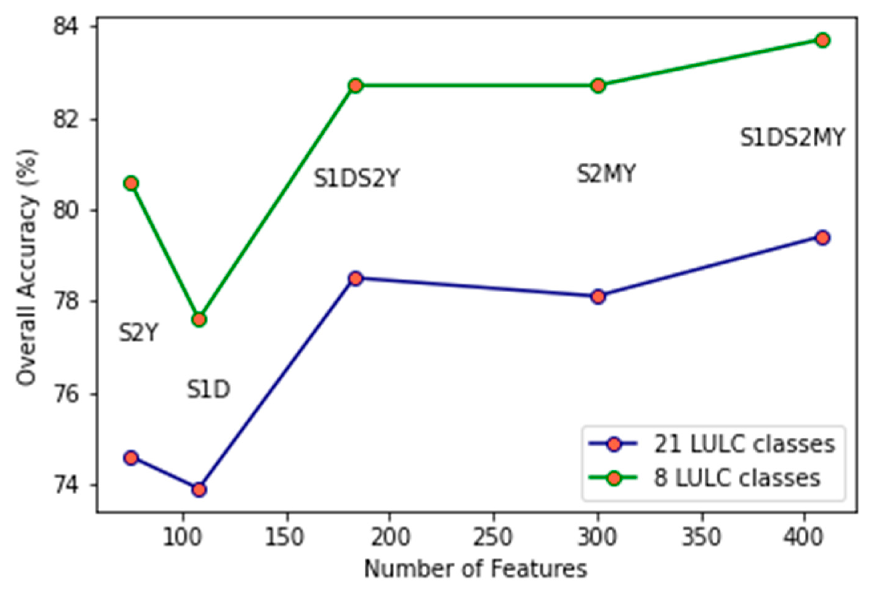
Table 6, the S1DS2MY feature set generates the highest OA (in both 21 and 8 classes) among the five evaluated feature sets, whereas the sole use of S1 data performs worst and leads to a drop of 5.5 percent points in accuracy using 21 LULC classes. The sole use of decadal S1 features (S1D) also performs worth than the yearly S2 data (S2Y).
In terms of computational requirements and accuracy, the use of yearly S2 data combined with decadal S1 data is outstanding (Figure 2). Indeed, using S1DS2Y still yields an OA of 78.3% (in 21 LULC classes) but only requires the calculation of 183 features (instead of 408 for the best-performing feature set).
The confusion matrix for the 21 LULC classes for the computationally efficient S1DS2Y feature set is summarized in Table A1 (in Appendix A) and shown in Table 7 when grouping the 21 classes into 8 broader classes. All results are based on the independent validation data. Using the detailed thematic classification with 21 classes, only 6 classes (Maize, Sugar beet, Sunflower, Rape and turnip rape, Woodland and Shrubland, and Grassland) obtained F1-scores above 79%. For seven classes (Rye, Oats, Rice, Triticale, Other root crops, and Fodder crops), the F1-scores were below 30, and the remaining 8 classes were between 30–70%. In cereal crops, Common wheat and Maize classes are well distinguished compared to other classes; however, some Common wheat samples are misallocated as Barley and Grassland. Moreover, the misclassified samples of the rest of the cereal crops mainly belong to the Common wheat and Grassland. In the other classes, some Potato samples are mixed with the Maize, and most points of Fodder crops are confused with Grassland.
Grouping the detailed classes into fewer broad classes increases the OA from 78.3% to 82.7%. High F1-scores (79.1–90.5%) were obtained for 5 of the 8 broad classes: Cereals, Root crops, Non-permanent industrial crops, Grassland, and Woodland and Shrubland, similar to [23]. For the three remaining classes, the UA was still acceptable (51.1–86.0%) but with generally insufficient PA (<30%). Overall, class 240 (Dry pulses, vegetables, and flowers) was the most difficult to separate (UA: 51.1%), probably due to the high intra-class thematic and spectral variability and very low number of training samples. Of the 5 broad crop classes, the class Cereals (210) performed best with an F1-score of 83.0%.

4. Discussion

Remote sensing has been a functional tool for large-scale crop mapping [50,51,52]. Monitoring using high-resolution remote sensing on broad areas is substantial for adjusting and optimizing agricultural production [53]. Comprehending crop patterns’ spatial and temporal variations is essential for assessing food security, policy application, and developing sustainable agricultural practices [54,55].
Google Earth Engine cloud-based computing platform, providing multi-sensor and multi-date satellite data, facilitates the generation of LULC maps over large areas and satisfies the needs of a wide range of applications such as cropland mapping and cost-effective monitoring.
This work is complementary to our previous study [23] and underlines the potential of using synergies between S1 and S2 data and using LUCAS field data for large-scale LULC classification.
Using solely S1 data, d’Andrimont et al. [22] reached an OA of 74.0% in classifying the same 21 classes. Their OA increases to 79.2% by grouping the detailed classes into 8 broader categories. In our previous study [23], we achieved an OA of 77.6% and 82.5% in classifying 21 and 8 classes, respectively, utilizing the SVM classifier while using solely S2 data.
As reported in Table 6, using only S1 features leads to an OA of 73.9%, which is almost identical to the results obtained by d’Andrimont et al. [22]. Utilizing S2 monthly and yearly indicators together produces a 3.7 percentage point increase in OA compared to using only S2 yearly indicators. Although adding S1 features to S2 monthly and yearly indicators (S1DS2MY) generates the highest OA between feature sets, the number of features increases considerably with an impact on computation cost and speed. The combination of decadal S1 and yearly S2 features, on the other hand, is computationally much more efficient and only results in a slight drop in accuracy of around one percentage point. Using this computationally efficient feature set (S1DS2Y), 19 field crops beside 2 broad classes containing Woodland and Shrubland and Grassland were classified with proper results. Both OA and class-specific F1-scores are analogous or better in some classes compared to S1 [22] and S2 [23] studies using similar training and validation data. By employing the S1DS2Y feature set, 21 classes were classified with an OA of 78.3% and the 8 groups with 82.7%. The feature set outperforms the mentioned studies utilizing RF classifiers using solely S1 or S2 features by 4.3 and 1.5 percentage points in OA, respectively.
Despite the very good temporal resolution of the S2 satellites, the acquisitions in 2018 were insufficient to produce cloud-free monthly composites for all of Europe. This caused missing values, especially in the winter and late fall months, which hampered the application of the RF classifier. This study used the median values of nine composites—with durations between one and three months—as “monthly” indicators to address this issue. Nevertheless, spectral values were unavailable for around 211,000 training samples (and 10,000 validation samples). Therefore, the cloud coverage issue prevented producing a full coverage map using S2 monthly features. In our recent study using S2 data, we used six (April–September) monthly features beside yearly centiles only for spectral indices. In this work, some extra indicators whose efficiency has been proven in [56] were calculated from spectral information and applied to the dataset. Moreover, S2 yearly centiles were calculated not only for spectral indices but also for all involved features.
Using S2 yearly indicators allows us to perfectly cover Europe, with, however, a 3.7 percentage point drop in the OA compared to S2MY, which also includes monthly composites. By adding weather-independent—but in itself less informative—S1 microwave features to S2 yearly indicators, a full coverage LULC map could be achieved with acceptable accuracy. Applying this method and according to Table 7, Cereals, Root crops, Non-permanent industrial crops, Grassland, and Woodland and Shrubland classes were well-classified by having F1-scores above 79% in grouped classes.
This is also shown with less detailed classes by Venter and Sydenham [21], who could improve the OA by 3 and 10 percentage points by combining S1 and S2 compared to the sole use of S2 and S1 data, respectively. Similar results were also obtained by Lechner et al. [57] for the detailed discrimination of tree species. They showed that S1 in combination with S2 shows an added value if only a few S2 data are available. As soon as an extensive multitemporal S2 dataset is available, the potential for improvement by S1 is drastically reduced.
In addition to high-quality remote sensing data, suitable reference data are essential for effective classification. Both quality and quantity play a pivotal role, as well as a good spatial distribution of the data. Here, the LUCAS dataset provides good reference data that have already been used in numerous recent papers for large-scale areas [18,19,20,21,22].

5. Conclusions

Earth observation (EO) data, such as the Copernicus Sentinel-1 (S1) and Sentinel-2 (S2) data, are instrumental for objective, timely, and cost-effective Land Use and Land Cover (LULC) mapping over large areas. However, data gaps due to clouds in S2 data and random noise in S1 data do not allow an easy wall-to-wall mapping for large areas. Moreover, although some datasets (i.e., LUCAS) are available as ground truth for training and evaluation of LULC maps, robust features that generalize well across space and time are still missing. This work introduced the potential of combining optical and radar data consisting of S2 yearly indicators and S1 10-day composites, achieving an overall accuracy (OA) of 78.3% for 19 crop types, plus Grassland and Woodland and Shrubland over 28 Member States of Europe. Although combining S1 and S2 features improved the accuracy slightly, merging S1 and S2 yearly features generates a full coverage map less dependent on cloud effects and satisfying OA.
Appropriate reference ground data are a crucial component for having a reliable classification. Therefore, the generation of the LULC map using the LUCAS dataset in the years when it is unavailable would be demanding. This issue could be addressed by finding relations between LUCAS 2018 and LUCAS 2022 (which have not been published yet) surveys using S1 and S2 EO data and applying machine learning methods.

Author Contributions

Conceptualization, F.V.; methodology, software, validation, formal analysis, B.G.; writing—original draft preparation, all authors; writing—review and editing, all authors; supervision, F.V., M.I. and C.A.; project administration, F.V.; funding acquisition, F.V. All authors have read and agreed to the published version of the manuscript.

Funding

This research was funded by the European Union’s Horizon 2020 Framework Programme for Research and Innovation under grant agreement No. 774234 (Landsupport) and No. 818346 (SIEUSOIL) and by the Austrian Research Promotion Agency (FFG) under the Austrian Space Applications Programme ASAP with the project number 878877 (ARmEO).

Institutional Review Board Statement

Not applicable.

Informed Consent Statement

Not applicable.

Data Availability Statement

The dataset d’Andrimont, Raphael (2020): LUCAS 2018 Copernicus was investigated in this research. The data are available in FigShare at https://doi.org/10.6084/m9.figshare.12382667.v3, accessed on 11 July 2022. The dataset d’Andrimont, Raphael; yordanov, momchil; Martinez-Sanchez, Laura; Eiselt, Beatrice; Palmieri, Alessandra; Dominici, Paolo; et al. (2020): Harmonised LUCAS in-situ land cover and use database for field surveys from 2006 to 2018 in the European Union was analyzed in this study. The data are available in FigShare at https://doi.org/10.6084/m9.figshare.9962765.v2, accessed on 11 July 2022.

Acknowledgments

This research was motivated by the need for detailed crop type maps that support different research activities and applications. For example, in the Horizon 2020 (H2020) Landsupport project (https://www.landsupport.eu, 12 July 2022), the development was driven by (1) the need for crop type maps for management, modeling, and scenario analysis for best practices in agriculture at the regional level, and (2) the need for spatially and thematically consistent European-wide land cover maps for the application of policy-related tools. In the context of the H2020 SIEUSOIL (https://www.sieusoil.eu, 12 July 2022), crop types, intensity and rotations are key indicators for designing optimal soil management practices. A more farmer-oriented application is being developed in the Austrian FFG ARmEO project, where maps are needed to run a benchmarking tool that will allow farmers to compare the performance of their crops against the same crop types growing on similar soils in the neighboring regions.

Conflicts of Interest

The authors declare no conflict of interest.

Appendix A

Table A1. The confusion matrix extracted from the RF classification result on validation data using the S1DS2Y feature set. UA = User Accuracy, PA = Producer’s Accuracy, OA = Overall Accuracy.
Code(211) Common Wheat(212) Durum Wheat(213) Barley(214) Rye(215) Oats(216) Maize(217) Rice(218) Triticale(219) Other Cereals(221) Potatoes(222) Sugar Beet(223) Other Root Crops(230) Other Non-Permanent(231) Sunflower(232) Rape and Turnip Rape(233) Soya(240) Dry Pulses, Vegetables,(250) Fodder Crops(290) Bare Arable Land(300) Woodland and Shrubland(500) GrasslandTotalUA
(%)
F1-Score
(%)
21143404058903082987692761816101144410226215063119510818153.063.9
2123530524117001000000002251601944568.538.6
21331997177391189613351208280250691052058182315656.254.5
2141201412752041020020202061822456.727.5
215801343200010000000065067542.77.3
2166314511315333149759932422423836892489414200434076.882.1
217000000300000000000100475.06.1
21800000000000000000000000.00.0
21900000000000000000000000.00.0
22100000101022552410712050226584.967.4
2222051151011057714341021130465488.288.3
223000000000001000000100250.02.0
2300000000000001030002140011093.646.5
231111029000172121535293362903470376.179.6
23211181060221625213031206102357153984.784.0
23300000000000010060002016493.851.5
2403740011021381371152193195323437851.135.1
25021103000000000006178101520786.015.7
2904514041000314231301626121114183673.239.5
30013367121273311451812911222242944311321730,473402735,50485.890.5
50046823143612820422614733812917493068161501398274129319,62724,76179.379.1
Total5401113433557018033778954541344036539733364215631697232058226131,82424,86781,448OA = 78.3%
PA (%)80.426.952.818.14.088.23.20.00.055.888.41.030.983.383.435.526.78.627.195.878.980.4

References

  1. Malinowski, R.; Lewiński, S.; Rybicki, M.; Gromny, E.; Jenerowicz, M.; Krupiński, M.; Nowakowski, A.; Wojtkowski, C.; Krupiński, M.; Krätzschmar, E.; et al. Automated Production of a Land Cover/Use Map of Europe Based on Sentinel-2 Imagery. Remote Sens. 2020, 12, 3523. [Google Scholar] [CrossRef]
  2. Topaloğlu, R.H.; Sertel, E.; Musaoğlu, N. Assessment of Classification Accuracies of SENTINEL-2 and LANDSAT-8 Data for Land Cover/Use Mapping. Int. Arch. Photogramm. Remote Sens. Spat. Inf. Sci. 2016, XLI-B8, 1055–1059. [Google Scholar] [CrossRef]
  3. Khatami, R.; Mountrakis, G.; Stehman, S.V. A meta-analysis of remote sensing research on supervised pixel-based land-cover image classification processes: General guidelines for practitioners and future research. Remote Sens. Environ. 2016, 177, 89–100. [Google Scholar] [CrossRef]
  4. European Commission. Trends in the EU Agricultural Land within 2015–2030. 2018. Available online: https://joint-research-centre.ec.europa.eu/document/download/cd9c4dfa-820b-445d-bcc5-bb6c46c4355a_en?filename=jrc113717.pdf (accessed on 11 July 2022).
  5. European Commission. Agri-Food Trade in 2018: Another Successful Year for Agri-Food Trade. 2019. Available online: https://ec.europa.eu/info/sites/info/files/food-farming-fisheries/news/documents/agri-food-trade-2018_en.pdf (accessed on 16 March 2021).
  6. Atzberger, C. Advances in Remote Sensing of Agriculture: Context Description, Existing Operational Monitoring Systems and Major Information Needs. Remote Sens. 2013, 5, 949–981. [Google Scholar] [CrossRef]
  7. Thenkabail, P. Remote Sensing of Global Croplands for Food Security; CRC Press: Boca Raton, FL, USA, 2009; ISBN 9781420090109. [Google Scholar]
  8. Inglada, J.; Arias, M.; Tardy, B.; Hagolle, O.; Valero, S.; Morin, D.; Dedieu, G.; Sepulcre, G.; Bontemps, S.; Defourny, P.; et al. Assessment of an Operational System for Crop Type Map Production Using High Temporal and Spatial Resolution Satellite Optical Imagery. Remote Sens. 2015, 7, 12356–12379. [Google Scholar] [CrossRef]
  9. Van der Velde, M.; van Diepen, C.A.; Baruth, B. The European crop monitoring and yield forecasting system: Celebrating 25 years of JRC MARS Bulletins. Agric. Syst. 2019, 168, 56–57. [Google Scholar] [CrossRef]
  10. Xiong, J.; Thenkabail, P.; Tilton, J.; Gumma, M.; Teluguntla, P.; Oliphant, A.; Congalton, R.; Yadav, K.; Gorelick, N. Nominal 30-m Cropland Extent Map of Continental Africa by Integrating Pixel-Based and Object-Based Algorithms Using Sentinel-2 and Landsat-8 Data on Google Earth Engine. Remote Sens. 2017, 9, 1065. [Google Scholar] [CrossRef]
  11. Defourny, P.; Bontemps, S.; Bellemans, N.; Cara, C.; Dedieu, G.; Guzzonato, E.; Hagolle, O.; Inglada, J.; Nicola, L.; Rabaute, T.; et al. Near real-time agriculture monitoring at national scale at parcel resolution: Performance assessment of the Sen2-Agri automated system in various cropping systems around the world. Remote Sens. Environ. 2019, 221, 551–568. [Google Scholar] [CrossRef]
  12. Hansen, M.C.; Loveland, T.R. A review of large area monitoring of land cover change using Landsat data. Remote Sens. Environ. 2012, 122, 66–74. [Google Scholar] [CrossRef]
  13. Brown, C.F.; Brumby, S.P.; Guzder-Williams, B.; Birch, T.; Hyde, S.B.; Mazzariello, J.; Czerwinski, W.; Pasquarella, V.J.; Haertel, R.; Ilyushchenko, S.; et al. Dynamic World, Near real-time global 10 m land use land cover mapping. Sci. Data 2022, 9, 251. [Google Scholar] [CrossRef]
  14. Immitzer, M.; Vuolo, F.; Atzberger, C. First Experience with Sentinel-2 Data for Crop and Tree Species Classifications in Central Europe. Remote Sens. 2016, 8, 166. [Google Scholar] [CrossRef]
  15. Phiri, D.; Simwanda, M.; Salekin, S.; Nyirenda, V.; Murayama, Y.; Ranagalage, M. Sentinel-2 Data for Land Cover/Use Mapping: A Review. Remote Sens. 2020, 12, 2291. [Google Scholar] [CrossRef]
  16. OneSoil. An AgriTech Start-Up from Belarus Demonstrates That Societal and Economic Benefits of Copernicus Go beyond the Borders of the European Union. Available online: https://www.copernicus.eu/en/news/news/observer-onesoil-a-copernicus-enabled-start-up-from-belarus (accessed on 11 July 2022).
  17. d’Andrimont, R.; Yordanov, M.; Martinez-Sanchez, L.; Eiselt, B.; Palmieri, A.; Dominici, P.; Gallego, J.; Reuter, H.I.; Joebges, C.; Lemoine, G.; et al. Harmonised LUCAS in-situ land cover and use database for field surveys from 2006 to 2018 in the European Union. Sci. Data 2020, 7, 352. [Google Scholar] [CrossRef] [PubMed]
  18. Close, O.; Benjamin, B.; Petit, S.; Fripiat, X.; Hallot, E. Use of Sentinel-2 and LUCAS Database for the Inventory of Land Use, Land Use Change, and Forestry in Wallonia, Belgium. Land 2018, 7, 154. [Google Scholar] [CrossRef]
  19. Pflugmacher, D.; Rabe, A.; Peters, M.; Hostert, P. Mapping pan-European land cover using Landsat spectral-temporal metrics and the European LUCAS survey. Remote Sens. Environ. 2019, 221, 583–595. [Google Scholar] [CrossRef]
  20. Weigand, M.; Staab, J.; Wurm, M.; Taubenböck, H. Spatial and semantic effects of LUCAS samples on fully automated land use/land cover classification in high-resolution Sentinel-2 data. Int. J. Appl. Earth Obs. Geoinf. 2020, 88, 102065. [Google Scholar] [CrossRef]
  21. Venter, Z.S.; Sydenham, M.A.K. Continental-Scale Land Cover Mapping at 10 m Resolution Over Europe (ELC10). Remote Sens. 2021, 13, 2301. [Google Scholar] [CrossRef]
  22. d′Andrimont, R.; Verhegghen, A.; Lemoine, G.; Kempeneers, P.; Meroni, M.; van der Velde, M. From parcel to continental scale—A first European crop type map based on Sentinel-1 and LUCAS Copernicus in-situ observations. Remote Sens. Environ. 2021, 266, 112708. [Google Scholar] [CrossRef]
  23. Ghassemi, B.; Dujakovic, A.; Żółtak, M.; Immitzer, M.; Atzberger, C.; Vuolo, F. Designing a European-Wide Crop Type Mapping Approach Based on Machine Learning Algorithms Using LUCAS Field Survey and Sentinel-2 Data. Remote Sens. 2022, 14, 541. [Google Scholar] [CrossRef]
  24. Drusch, M.; Del Bello, U.; Carlier, S.; Colin, O.; Fernandez, V.; Gascon, F.; Hoersch, B.; Isola, C.; Laberinti, P.; Martimort, P.; et al. Sentinel-2: ESA′s Optical High-Resolution Mission for GMES Operational Services. Remote Sens. Environ. 2012, 120, 25–36. [Google Scholar] [CrossRef]
  25. Gorelick, N.; Hancher, M.; Dixon, M.; Ilyushchenko, S.; Thau, D.; Moore, R. Google Earth Engine: Planetary-scale geospatial analysis for everyone. Remote Sens. Environ. 2017, 202, 18–27. [Google Scholar] [CrossRef]
  26. Amani, M.; Mahdavi, S.; Afshar, M.; Brisco, B.; Huang, W.; Mohammad Javad Mirzadeh, S.; White, L.; Banks, S.; Montgomery, J.; Hopkinson, C. Canadian Wetland Inventory using Google Earth Engine: The First Map and Preliminary Results. Remote Sens. 2019, 11, 842. [Google Scholar] [CrossRef]
  27. Thanh Noi, P.; Kappas, M. Comparison of Random Forest, k-Nearest Neighbor, and Support Vector Machine Classifiers for Land Cover Classification Using Sentinel-2 Imagery. Sensors 2017, 18, 18. [Google Scholar] [CrossRef] [PubMed]
  28. D’Andrimont, R.; Verhegghen, A.; Meroni, M.; Lemoine, G.; Strobl, P.; Eiselt, B.; Yordanov, M.; Martinez-Sanchez, L.; van der Velde, M. LUCAS Copernicus 2018: Earth-observation-relevant in situ data on land cover and use throughout the European Union. Earth Syst. Sci. Data 2021, 13, 1119–1133. [Google Scholar] [CrossRef]
  29. Bouhennache, R.; Bouden, T.; Taleb-Ahmed, A.; Cheddad, A. A new spectral index for the extraction of built-up land features from Landsat 8 satellite imagery. Geocarto Int. 2019, 34, 1531–1551. [Google Scholar] [CrossRef]
  30. Rikimaru, A.; Roy, P.S.; Miyatake, S. Tropical forest cover density mapping. Trop. Ecol. 2002, 43, 39–47. [Google Scholar]
  31. Jacques, D.C.; Kergoat, L.; Hiernaux, P.; Mougin, E.; Defourny, P. Monitoring dry vegetation masses in semi-arid areas with MODIS SWIR bands. Remote Sens. Environ. 2014, 153, 40–49. [Google Scholar] [CrossRef]
  32. Le Maire, G.; François, C.; Dufrêne, E. Towards universal broad leaf chlorophyll indices using PROSPECT simulated database and hyperspectral reflectance measurements. Remote Sens. Environ. 2004, 89, 1–28. [Google Scholar] [CrossRef]
  33. Wulf, H.; Stuhler, S. Sentinel-2: Land Cover, Preliminary User Feedback on Sentinel-2A Data. In Proceedings of the Sentinel-2A Expert Users Technical Meeting, Frascati, Italy, 29–30 September 2015; pp. 29–30. [Google Scholar]
  34. Xu, H. Modification of normalised difference water index (NDWI) to enhance open water features in remotely sensed imagery. Int. J. Remote Sens. 2006, 27, 3025–3033. [Google Scholar] [CrossRef]
  35. Vogelmann, J.E.; Rock, B. Spectral characterization of suspected acid deposition damage in red spruce (Picea Rubens) stands from Vermont. In Proceedings of the Airborne Imaging Spectrometer Data Anal, Workshop, Pasadena, CA, USA, 8–10 April 1985; pp. 51–55. [Google Scholar]
  36. Zha, Y.; Gao, J.; Ni, S. Use of normalized difference built-up index in automatically mapping urban areas from TM imagery. Int. J. Remote Sens. 2003, 24, 583–594. [Google Scholar] [CrossRef]
  37. Van Deventer, A.P.; Ward, A.D.; Gowda, P.H.; Lyon, J.G. Using thematic mapper data to identify contrasting soil plains and tillage practices. Photogramm. Eng. Remote Sens. 1997, 63, 87–93. [Google Scholar]
  38. Kriegler, F.J.; Malila, W.A.; Nalepka, R.F.; Richardson, W. Preprocessing Transformations and Their Effects on Multispectral Recognition. Remote Sens. Environ. 1969, VI, 97–131. [Google Scholar]
  39. Gao, B. NDWI—A normalized difference water index for remote sensing of vegetation liquid water from space. Remote Sens. Environ. 1996, 58, 257–266. [Google Scholar] [CrossRef]
  40. Huete, A. A soil-adjusted vegetation index (SAVI). Remote Sens. Environ. 1988, 25, 295–309. [Google Scholar] [CrossRef]
  41. Blackburn, G.A. Quantifying Chlorophylls and Caroteniods at Leaf and Canopy Scales. Remote Sens. Environ. 1998, 66, 273–285. [Google Scholar] [CrossRef]
  42. Radoux, J.; Chomé, G.; Jacques, D.; Waldner, F.; Bellemans, N.; Matton, N.; Lamarche, C.; d’Andrimont, R.; Defourny, P. Sentinel-2’s Potential for Sub-Pixel Landscape Feature Detection. Remote Sens. 2016, 8, 488. [Google Scholar] [CrossRef]
  43. Breiman, L. Random Forests. Mach. Learn. 2001, 45, 5–32. [Google Scholar] [CrossRef]
  44. Vapnik, V. The Nature of Statistical Learning Theory; Springer Science & Business Media: Berlin/Heidelberg, Germany, 1999; ISBN 9780387987804. [Google Scholar]
  45. Vapnik, V.N. The Nature of Statistical Learning Theory, 2nd ed.; Springer: New York, NY, USA, 2000; ISBN 9781475732641. [Google Scholar]
  46. Chen, T.; Guestrin, C. XGBoost. In Proceedings of the 22nd ACM SIGKDD International Conference on Knowledge Discovery and Data Mining, KDD ’16, San Francisco, CA, USA, 13–17 August 2016; Krishnapuram, B., Shah, M., Smola, A., Aggarwal, C., Shen, D., Rastogi, R., Eds.; ACM: New York, NY, USA, 2016; pp. 785–794, ISBN 9781450342322. [Google Scholar]
  47. McCulloch, W.S.; Pitts, W. A logical calculus of the ideas immanent in nervous activity. Bull. Math. Biophys. 1943, 5, 115–133. [Google Scholar] [CrossRef]
  48. Abdi, A.M. Land cover and land use classification performance of machine learning algorithms in a boreal landscape using Sentinel-2 data. GIScience Remote Sens. 2020, 57, 1–20. [Google Scholar] [CrossRef]
  49. Pedregosa, F.; Varoquaux, G.; Gramfort, A.; Michel, V.; Thirion, B.; Grisel, O.; Blondel, M.; Prettenhofer, P.; Weiss, R.; Dubourg, V.; et al. Scikit-learn: Machine Learning in Python. J. Mach. Learn. Res. 2011, 12, 2825–2830. [Google Scholar]
  50. Gallego, F.J.; Kussul, N.; Skakun, S.; Kravchenko, O.; Shelestov, A.; Kussul, O. Efficiency assessment of using satellite data for crop area estimation in Ukraine. Int. J. Appl. Earth Obs. Geoinf. 2014, 29, 22–30. [Google Scholar] [CrossRef]
  51. Thenkabail, P.S.; Wu, Z. An Automated Cropland Classification Algorithm (ACCA) for Tajikistan by Combining Landsat, MODIS, and Secondary Data. Remote Sens. 2012, 4, 2890–2918. [Google Scholar] [CrossRef]
  52. Wu, W.; Shibasaki, R.; Yang, P.; Zhou, Q.; Tang, H. Remotely sensed estimation of cropland in China: A comparison of the maps derived from four global land cover datasets. Can. J. Remote Sens. 2008, 34, 467–479. [Google Scholar] [CrossRef]
  53. Jiang, Y.; Lu, Z.; Li, S.; Lei, Y.; Chu, Q.; Yin, X.; Chen, F. Large-Scale and High-Resolution Crop Mapping in China Using Sentinel-2 Satellite Imagery. Agriculture 2020, 10, 433. [Google Scholar] [CrossRef]
  54. Liu, Z.; Yang, P.; Wu, W.; You, L. Spatiotemporal changes of cropping structure in China during 1980–2011. J. Geogr. Sci. 2018, 28, 1659–1671. [Google Scholar] [CrossRef]
  55. Tang, H.; Wu, W.; Yang, P.; Li, Z. Systematic Synthesis of Impacts of Climate Change on China′s Crop Production System. J. Integr. Agric. 2014, 13, 1413–1417. [Google Scholar] [CrossRef]
  56. Immitzer, M.; Neuwirth, M.; Böck, S.; Brenner, H.; Vuolo, F.; Atzberger, C. Optimal Input Features for Tree Species Classification in Central Europe Based on Multi-Temporal Sentinel-2 Data. Remote Sens. 2019, 11, 2599. [Google Scholar] [CrossRef]
  57. Lechner, M.; Dostálová, A.; Hollaus, M.; Atzberger, C.; Immitzer, M. Combination of Sentinel-1 and Sentinel-2 Data for Tree Species Classification in a Central European Biosphere Reserve. Remote Sens. 2022, 14, 2687. [Google Scholar] [CrossRef]
Figure 1. The main steps for the classification procedure.
Land 11 01397 g001
Figure 2. The relation of overall accuracy with the number of features in five different feature sets using 21 and 8 LULC classes.
Land 11 01397 g002
Table 1. The classification scheme adapted from [22] with 19 crop types plus 2 broad categories with Woodland and Shrubland and Grassland classes. The “Main Class Name”, with the respective class codes (“Code”), was used in this research.
Grouped Class NameCodeMain Class NameClass Descriptors in LUCAS Level-3 Landcover
Cereals211Common wheatB11-Common wheat
212Durum wheatB12-Durum wheat
213BarleyB13-Barley
214RyeB14-Rye
215OatsB15-Oats
216MaizeB16-Maize
217RiceB17-Rice
218TriticaleB18-Triticale
219Other cerealsB19-Other cereals
Root crops221PotatoesB21-Potatoes
222Sugar beetB22-Sugar beet
223Other root cropsB23-Other root crops
Non-permanent industrial crops230Other non-permanent industrial cropsB34-Cotton|B35-Other fibre and oleaginous crops|B36-Tobacco|B37-Other non-permanent industrial crops
231SunflowerB31-Sunflower
232Rape and turnip rapeB32-Rape and turnip rape
233SoyaB33-Soya
Dry pulses, vegetables, and flowers240Dry pulses, vegetables, and flowersB41-Dry pulses|B43-Other fresh vegetables|B44-Floriculture and ornamental plants|B45-Strawberries
Fodder crops250Fodder cropsB51-Clovers|B52-Lucerne|B53-Other leguminous and mixtures for fodder|B54-Mixed cereals for fodder
Bare arable land290Bare arable landF40-Other bare soil (only with U111/112/113 Land use)
Woodland and Shrubland300Woodland and ShrublandB71-Apple fruit|B72-Pear fruit|B73-Cherry fruit|B74-Nuts trees|B75-Other fruit trees and berries|B76-Oranges|B77-Other citrus fruit|B81-Olive groves|B82-Vineyards|B83-Nurseries|B84-Permanent industrial crops|C10-Broadleaved woodland|C21-Spruce dominated coniferous woodland|C22-Pine dominated coniferous woodland|C23-Other coniferous woodland|C31-Spruce dominated mixed woodland|C32-Pine dominated mixed woodland|C33-Other mixed woodland|D10-Shrubland with sparse tree cover|D20-Shrubland without tree cover
Grassland500GrasslandB55-Temporary grasslands|E10-Grassland with sparse tree/shrub cover|E20-Grassland without tree/shrub cover|E30-Spontaneously vegetated surfaces
Table 2. Spectral bands and indices extracted from S2 and used for LULC classification.
Feature NameDescription
Spectral BandsB2: BlueB7: Red Edge 3
B3: GreenB8: NIR
B4: RedB8A: NIR narrow
B5: Red Edge 1B11: SWIR 1
B6: Red Edge 2B12: SWIR 2
Spectral Indices BLFEI :   ( ( ( B 3 + B 4 + B 12 ) / 3 ) B 11 ) / ( ( ( B 3 + B 4 + B 12 ) / 3 ) + B 11 )
BSI: ( ( B 11 + B 4 ) ( B 8 + B 2 ) ) / ( ( B 11 + B 4 ) + ( B 8 + B 2 ) )
DIRESWIR :   B 4 B 11
GI :   B 3 / B 4
LCCI :   B 7 / B 5
MNDWI :   ( ( B 3 B 11 ) ) / ( ( B 3 + B 11 ) )
MSI :   B 11 / B 8
NDBI :   ( ( B 11 B 8 ) ) / ( ( B 11 + B 8 ) )
NDRESWIR :   ( ( B 6 B 12 ) ) / ( ( B 6 + B 12 ) )
NDTI :   ( ( B 11 B 12 ) ) / ( ( B 11 + B 12 ) )
NDVI :   ( ( B 8 B 4 ) ) / ( ( B 8 + B 4 ) )
NDWI 1 :   ( ( B 8 B 11 ) ) / ( ( B 8 + B 11 ) )
SAVI :   ( ( B 8 B 4 ) ) / ( ( B 8 + B 4 + 0.5 ) ) 1.5
SRNIRR :   B 8 / B 4
SRNIRRE 2 :   B 8 / B 6
Abbreviations: NIR = near Infrared; SWIR = shortwave infrared; BLFEI = built-up land features extraction index; BSI = bare soil index; DIRESWIR = red SWIR1 difference; GI = greenness index; LCCI = leaf chlorophyll content index; MNDWI = modified normalized difference water index; MSI = moisture stress index; NDBI = normalized difference built-up index; NDRESWIR = normalized difference red-edge and SWIR2; NDTI = normalized difference tillage index; NDVI = normalized difference vegetation index; NDWI1 = normalized difference water index 1; SAVI = soil adjusted vegetation index; SRNIRR = NIR and red ratio; SRNIRRE2 = NIR and RE2 ratio.
Table 3. Microwave indicators derived from S1 in the year 2018 and used for LULC classification.
Feature NameDescription
Microwave featuresVV: Single co-polarization, vertical transmit/vertical receive
VH: Dual-band cross-polarization, vertical transmit/horizontal receive
CR: VH/VV (cross-polarization ratio)
Table 4. The number of samples with missing values for each monthly feature. “Med” indicates the median value.
Month (2018)JanuaryFebruaryMarchAprilMayJuneJulyAugustSeptemberOctoberNovemberDecember
Missing values360,219187,287195,53014,20117,86624,34710,97347,11287579763191,106503,723
Utilized featuresMed (January, February, March)AprilMayJuneJulyAugustSeptemberOctoberMed (November and December)
Table 5. Process of extracting validation samples from LUCAS core points.
SituationNumber of Samples
Total LUCAS core points333,854
Remaining after keeping points directly interpreted in the field238,961
Remaining after keeping points within parcels greater than 0.5 ha177,609
Remaining after eliminating points surveyed in the Copernicus module122,070
Remaining after keeping points with a homogeneous land cover98,146
Remaining after keeping points related to the classification scheme91,201
Table 6. Five different input data scenarios generated from S1 and S2 features. Shown are the number of training and validating samples as well as the number of features. Moreover, the overall accuracy (OA) of applying an RF classifier on different feature sets (using all 21 and 8 aggregated LULC classes) and evaluating with validation data are displayed.
Feature SetAbbreviationNumber of Training SamplesNumber of Validating SamplesNumber of FeaturesOA (21 Classes)OA (8 Classes)
S1 Decadal + S2 Monthly and Yearly featuresS1DS2MY1,749,60481,44840879.4%83.7%
S1 Decadal + S2 Yearly featuresS1DS2Y1,950,92281,44818378.3%82.7%
S2 Monthly and Yearly featuresS2MY1,749,61481,44830078.1%82.7%
S2 Yearly featuresS2Y1,950,93281,4487574.4%80.5%
S1 Decadal featuresS1D1,950,92281,44810873.9%77.6%
Table 7. Confusion matrix for comprehensive classes by applying a trained model (using RF classifier) on the validation dataset utilizing S1DS2Y feature set. UA = User Accuracy, PA = Producer’s Accuracy, OA = Overall Accuracy.
Comprehensive ClassCode210220230240250290300500TotalUAF1-Score
Cereals21013,3911883602273349584292516,42581.5%83.0%
Root crops220188342033190692190.6%80.4%
Non-permanent industrial crops230452920425513137392241684.5%79.7%
Dry pulses, vegetables and flowers240183425193195323437851.1%35.1%
Fodder crops2507006178101520786.0%15.7%
Bare arable land290288181626121114183673.2%39.5%
Woodland and Shrubland30053022794311321730,473402735,50485.8%90.5%
Grassland5001818381631501398274129319,62724,76179.3%79.1%
Total15,855115327077232058226131,82424,86781,448OA = 82.7%
PA84.5%72.3%75.4%26.7%8.6%27.1%95.8%78.9%
Publisher’s Note: MDPI stays neutral with regard to jurisdictional claims in published maps and institutional affiliations.

