Delineation of the Development Boundary of the Central District of Zhengzhou, China

Abstract

An urban development boundary is an effective means to guide urban development and restrain unplanned expansion of urban space. Scientifically-based delineation and control of the boundary can help with sustainable use of land resources and better spatial planning. This study took land use data from 2000, 2010, and 2020 for the central urban area of Zhengzhou and predicted the land use pattern in 2035. We used auto-logistic selection of driving factors, future land use simulation, and system dynamics models to delineate the development boundary of the central urban area. We complemented and optimized the boundary using agricultural and ecological perspectives. The results indicated the following: (1) The ROC values of land driving factors were greater than 0.75 in the regression test, and the Kappa and OA were greater than 0.92 in the accuracy test of land simulation results. (2) The boundary range initially delineated based on morphology was 2319 km². There was a clear overall development trend of the central urban area to the east and southeast, which included the historical urban area of Zhengzhou and the new government planning area. (3) The optimized boundary of the central district area was 2209 km², the ecological land control area was 136 km², and the basic farmland protection area was 54 km². The Yellow River, the airport, and the western, southern, and eastern areas were already formed. The study concluded that the delineated boundary was in line with the scientific concepts of ‘rigid’ and ‘flexible’ factors, which have positive effects on the protection of arable land resources and ecological land, as well as meeting the needs of urban development. The level of sustainable development of the region was effectively improved.

1. Introduction

Since the 21st century, China’s urbanization has entered a rapid development stage and the spatial scale of cities has expanded, with many cities spreading in a ‘pancake’ style, which is an inefficient use of land resources and disorderly construction [1]. The unplanned growth of land for construction has led to the erosion of the ecological base of cities and a serious imbalance between urban and rural development [2]. An urban development boundary (UDB), also known as an urban growth boundary, is an important means to balance the social, economic, and ecological environment; optimize the structure of land use; and achieve sustainable development [3]. A UBD can effectively prevent a series of problems including environmental damage and traffic congestion caused by ‘big city disease’ [4]. For China, the scientific definition of the UDB and the coordination of land for ecological protection, basic agriculture, and construction and development are important issues to be solved in the spatial planning of national land allocation [5].

The UDB concept originated from Howard’s ‘idyllic city theory’ in the 19th century. By the 1930s, the British Greater London District Plan used the urban periphery green belt as a physical boundary to limit urban sprawl [6]; this was the initial exploration of boundary delineation. The concept of boundaries was then formally introduced in the United States under the ‘New Urbanism’ school of thought to limit the scale of spatial expansion by delineating suburban and urban boundaries [7]. At the end of the 20th century, theories of compact cities and smart growth were proposed [8], and the link between urban boundaries and land expansion began to be strengthened [9].

It is always a critical goal to achieve urban renewal and curb urban sprawl in all developed or capitalist countries. The original cities experiencing urban sprawl were the US’s central and western emerging cities. This urban sprawl pattern expanded rapidly to Latin America, then Asia, and eventually became a global phenomenon [10]. On the other hand, most European cities had developed differently from those in America and Asia, generally adhering to a monocentric growth pattern with an apparent hierarchy of centers and sub-centers, with expansion gathered around a dense historical center and its commercial and business expansion. There is an obvious political–administrative fragmentation in Italy’s urban system [11]. Each city still designs its spatial development program independently, showing distinct social fragmentation, and significantly reducing social interaction and learning. In Spain, the distribution and expansion of cities led to a more considerable concentration of population, high heterogeneity of sprawl, and more dispersed industrial sites, etc. [12]. In France, the decentralization rate decreased with urban growth, but the commuting distance of residents of polycentric areas did not systematically decrease, and the average distance from households to the city center increased [13].

Moreover, many North American policies, such as the revitalization of urban centers, mixed-use urban regeneration plans for inner cities, and controlled sprawl growth boundaries, found their counterparts in European and especially British planning policies. The concepts of compact cities and controlled urban sprawl were a focused and growing topic of discussion among the British and European commentators on planning. Undoubtedly, the urban sprawl in the UK was strictly controlled, performing particularly effectively in major northern cities such as Liverpool [14]. However, the population density in the UK will decrease due to housing costs and demand, which could increase the social isolation between the compact urban core and the expanding suburbs/periphery. In Germany, urban sprawl was most likely a product of specific legislative and political circumstances [15]. The urban sprawl generally occurred with a shrinking population (some of them due to the shrinking economy), which implies that enhanced state intervention could guide the spatial development with the most remarkable capacity. However, this may lead to a widespread ‘perforation’ of German cities, as only those selected urban areas, particularly the most successful inner cities of the urban areas, are most likely to experience stabilization and further improvement.

Urban sprawl in Europe is influenced significantly by public policy and the public sector. Whether the policies can further promote compact and enclosed cities without adverse social consequences depends partly on whether housing costs follow the changes in housing demand [16]. However, urban renewal has been used in some North American and Europe countries as a compromise with the ‘real estate boom’ under capitalist interference [17]. Real estate development is a considerable economic influence that has terribly impacted wage-earning class communities and the essential availability of housing. Capitalism drives and forces people into those emerging cities where houses cannot be considered homes but just boxes where people can barely survive and work [18]. This type of urban sprawl significantly increases social inequality and has horrible effects on the sustainable urban development of a country or region.

In 2006, China promulgated the Measures for the Preparation of Urban Planning [19], which first proposed studying the spatial development boundary of central urban areas. Following this, many studies have examined the delineation of the UDB. Nowadays, the main delineation types are stable control, accelerated integration, and comprehensive coordination [20]. The stable control approach concentrates on the bottom-line protection of urban ecology and arable land. The analysis focuses on the distribution of farmland [21], landscape pattern [22], and habitat quality [23,24], and it uses an ‘anti-planning’ idea to define the scope of construction land development [25]. Accelerated integration is based on ecological protection, regulating the spatial competition between rural land and urban land [26], and using population and economic data to identify the expansion intensity and direction of construction land [27]. Comprehensive coordination focuses on the balance between urban development and the ecological bottom line, mostly using the method of setting ‘flexible’ boundaries in the development reserve area and ‘rigid’ boundaries in the ecological red line area [28], which provides a hierarchical and classified analysis of the ‘demolition’ or ‘retention’ of construction land.

The delineation of the UDB based on the predictive simulation of land use patterns is a common method in Chinese and international studies. Among the analytical models for land use/cover change (LUCC), the most common are CLUEs [29], cellular automata (CA) [30] and artificial neural networks (ANNs) [31]. The most common land demand forecasting methods are gray system models [32], Markov chains [33], and system dynamics (SD) [34]. The future land use simulation (FLUS) model is also widely used in many studies [35,36,37,38]. 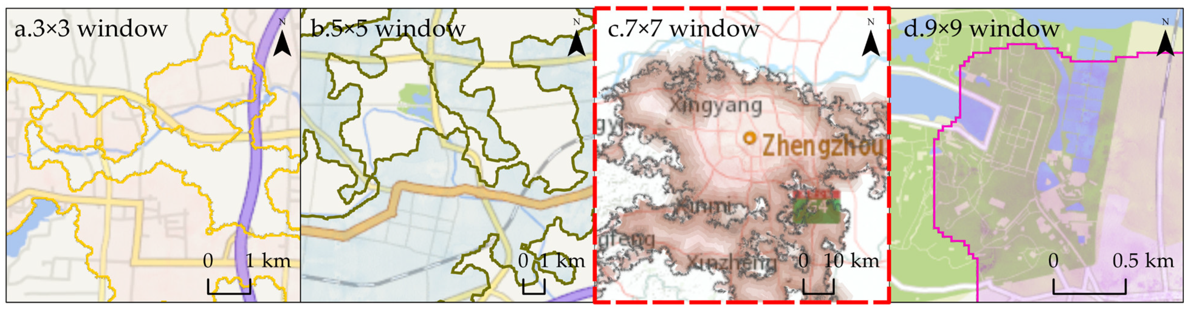Its adaptive inertia mechanism for roulette selection of land patches can simulate the coupled complexity of human social activities and the natural environment to identify future land use patterns with high accuracy [39,40]. The FLUS model can also be coupled with the morphological expansion and the erosion method (MED) to delineate the boundaries of land classes in different neighborhood windows based on the simulation results. Currently, in studies of UDB delineation at the municipal scale [27,36,41], the scope for expansion owing to rigid intra-city demand cannot break through the fixed administrative boundaries. Thus, small-scale land simulations differ greatly from the actual land class competition and policy directions. This results in ongoing conflict between boundary delineation results and the maintenance of land planning trajectories. By excluding the constraining influence of administrative scope on urban expansion and defining the variable relationship of land competition, a level of objectivity and planning can be brought to the delineation of the UDB.

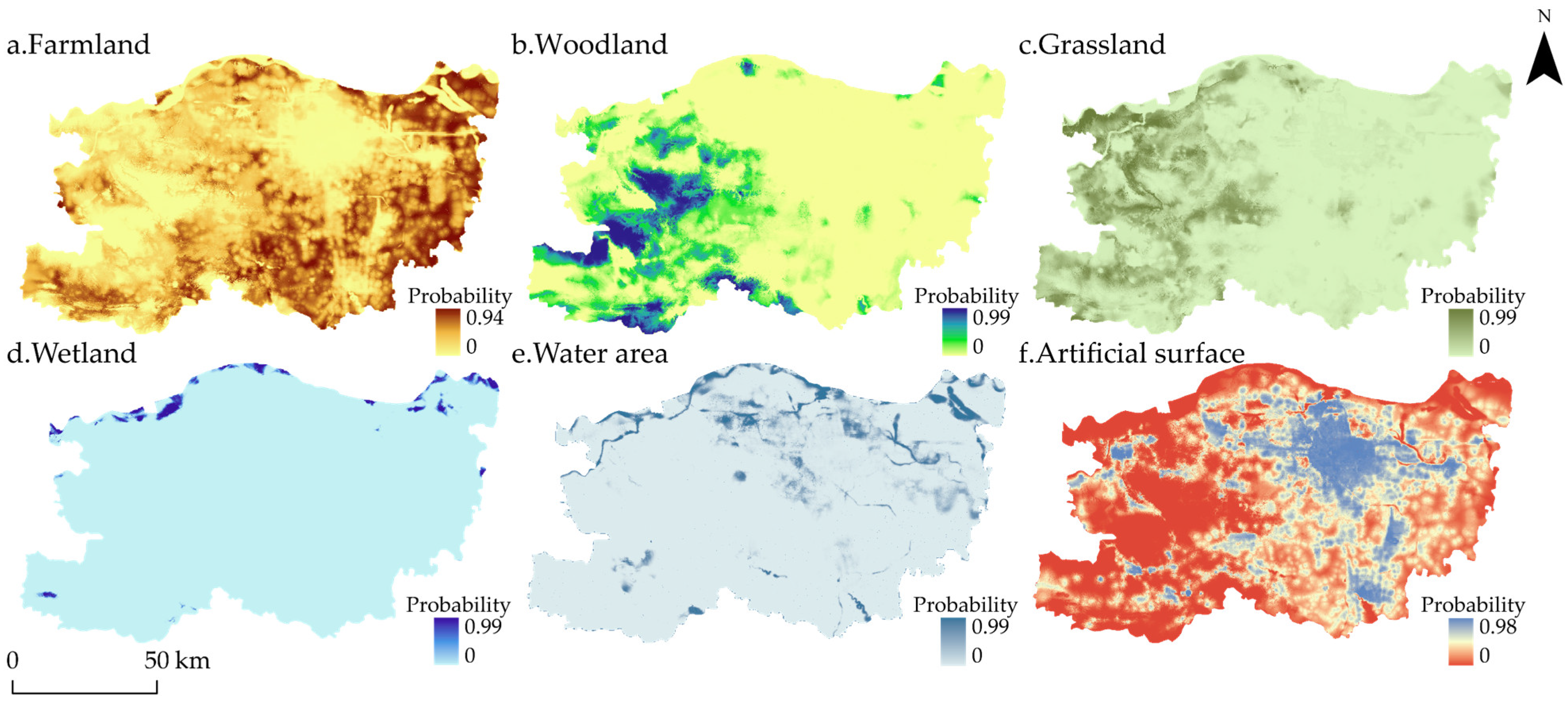
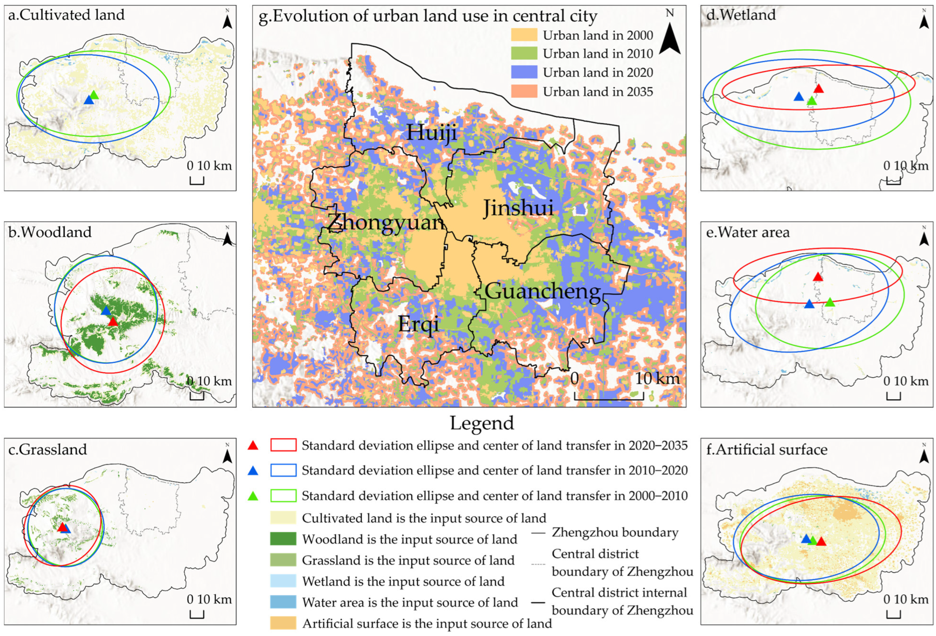
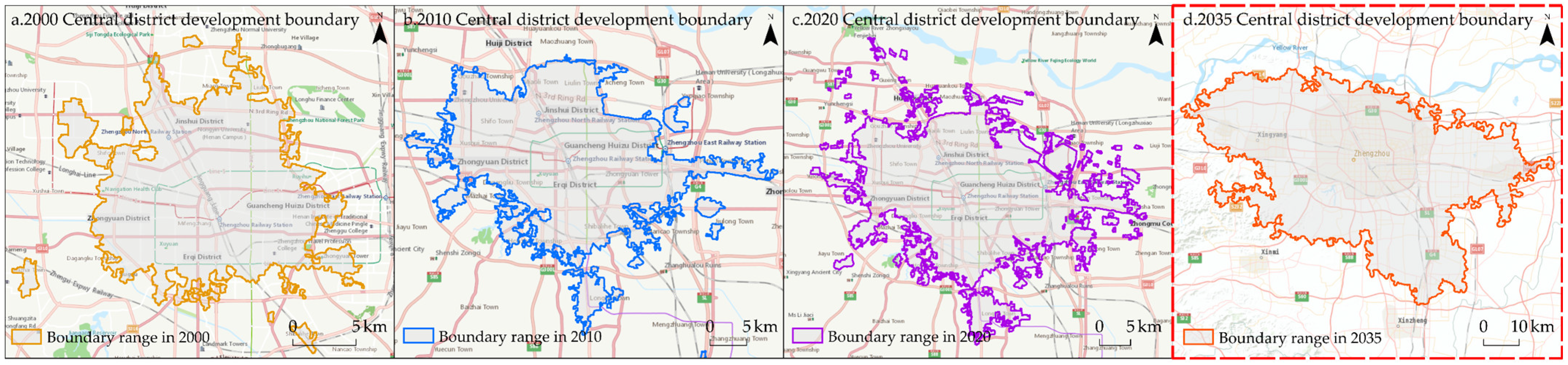
Zhengzhou is the capital city of Henan Province with a population of hundreds of millions; its urban spatial expansion is essential for economic development and accessibility. A UDB can effectively help the management of the spatial structure and smart growth of Zhengzhou to prevent the unplanned expansion of urban land, highlight the risk factors of ‘big city disease’, and promote the ecological protection and rational development of the Yellow River basin. On this basis, the current study took the whole city of Zhengzhou as the unit of analysis and focused on the concept of upper-level design guiding lower-level planning to delineate the development boundary of the central district to balance peripheral expansion and region-wide coordination. The land use data for three time points (2000, 2010 and 2020) were selected, and an auto-logistic model was used to screen the correlation of driving factors, an SD model was used to calculate the demand for different types of land development, and the FLUS model was used to predict the future land use pattern under the comprehensive development scenario. Finally, the MED method was applied to delineate and optimize the development boundary.

Therefore, the following sub-objectives of this paper are proposed: (1) to conduct a linear regression analysis of the driving factors that promote land or urban land use change, and this analysis enables the study to consider the influence of physical geography, location conditions, and socio-economic factors, which provides driving circumstances for the simulation prediction of subsequent research and improves the comprehensiveness and rigor of results; and (2) to conduct a simulation and prediction of future land use patterns. The reasonable results of future construction land prediction will be an important reference for delineating the UDB. With the method combining the historical land patterns and future changes, the degree and direction of urban expansion were expressed in a spatial form. It provided a scientific basis for urban renewal and boundary delimitation. (3) Delineate the UGB of the core zone of Zhengzhou and optimize the limited urban expansion by analyzing the interference of the ecological environment and agricultural production on the boundary to permit urban expansion within a specific reasonable range to achieve the optimal sustainable development. The paper mainly provides a systematic process for delineating the UDB: driving force action, land simulation prediction, and boundary definition and adjustment. The research system and theory breaks through the obstacles of public policies on urban development, which not only meet the rigid demands of residents but also realize the renewal and further development of the city and do not violate the law of natural growth. This study provides a technical reference for delineating the development boundaries of global cities, urban agglomerations, and even larger scales. It provides a vital basis for those urban decision-makers to allocate public service resources and realize the prospective development of construction land.

2. Study Area and Material

2.1. Study Area

Zhengzhou is located in the transition zone between the middle and lower reaches of the Yellow River and the northeastern flank of the Funiu Mountains to the Huang Huai Plain (112°42′−114°14′ E, 34°16′−34°58′ N) (Figure 1). Zhengzhou is an important national hub for railroads, airlines, postal services, and electrical power. It is the capital of Henan Province, the core city of the Central Plains City Cluster, and one of the nine national central cities in China. It has six municipal districts, five county-level cities, and one county under its jurisdiction. The spatial area of the city is 7446 km², of which the built-up area of the city is 1181 km² and the built-up area of the central district is 651 km². The gross domestic product (GDP) of Zhengzhou in 2020 was USD 179 billion, the resident population was 12.6 million, and the urbanization rate was 78%. The ecological protection and high-quality development strategy of the Yellow River Basin has led to additional requirements for the development of Zhengzhou; therefore, the scientific delineation of the development boundary of the central urban area is important for weighing local economic development and ecological protection.

2.2. Data and Preprocessing

The research data in this study included land use, topography and geomorphology, nature, society, and location. The specific sources are shown in

Table 1. Information on data sources.

Data Attribute	Data Name	Data Source
Basic data	Administrative divisions of Henan province and Zhengzhou City	Resource and Environment Science and Data Center (http://www.resdc.cn/, accessed on 1 August 2021)
	Land use data of Zhengzhou (30 m)	GlobeLand30 (http://globallandcover.com/, accessed on 5 August 2021)
Topography	DEM (30 m)	Geographical Information Monitoring Cloud Platform (http://www.dsac.cn/, accessed on 5 August 2021)
	Slope	Slope is calculated by DEM and ArcGIS tools
Natural factors	Soil texture	Resource and Environment Science and Data Center (accessed on 5 August 2021)
	Mean annual precipitation	China Meteorological Administration (http://www.cma.gov.cn/en2014/, accessed on 5 August 2021)
Social factors	Night light	National Centers for Environmental Information (https://www.ngdc.noaa.gov/, accessed on 10 August 2021)
	Population, GDP density	Zhengzhou city bureau of statistics (http://tjj.zhengzhou.gov.cn/, accessed on 12 August 2021)Statistical Yearbook of CNKI (https://www.cnki.net/, accessed on 12 August 2021)
Geographical factors	Road network (provincial road, national road, highway, city road)	Open Street Map (http://www.openstreetmap.org/, accessed on 15 August 2021)
	Bus routes
	The rail network
	River, water surface	Resource and Environment Science and Data Center (accessed on 15 August 2021)
	Residential areas
	POI

, where points of interest (POI) data include shopping malls, hotels, hospitals, banks, parks, squares, residential areas, educational institutions, and public facilities. The original land use data were divided into six categories: cultivated land, woodland, grassland, wetland, water area, and artificial surface. Night light data were corrected for intensity saturation. The raster data used in the study were all unified at 30 m × 30 m resolution, the geographical coordinate system was GCS_WGS_1984, and the projected coordinate system was WGS_1984_UTM_Zone_49N.

3. Methodology

3.1. Selection of Auto-Logistic Drivers

Logistic regression models are a categorical statistical method used to measure the nonlinear relationship between dependent and independent variables. The results indicate the probability size of the relationship, but they require a normal distribution in the mathematical sense, and they cannot show the drivers brought by the spatial expansion and geographical elements [42]. Therefore, this study established an auto-logistic model with spatial attributes by assigning a spatial autocorrelation weight function and combining the homogeneity and independence of the logistic model. The formula is as follows:

$$Pro\left(Re{f}_n=1|{\alpha }_0, \alpha , a\right)=\frac{\exp {\alpha }_0+{\alpha }_1^{’}{\beta }_n+a\sum W_{mn}}{1+\exp {\alpha }_0+{\alpha }_1^{’}{\beta }_n+a\sum W_{mn}}$$

(1)

where pro is the probability of event occurrence; Ref_n is the reference variable; α is the probability of event occurrence; β_n is the independent variable; a is the covariate coefficient; and W_mn is the weight function of spatio-temporal points m and n. The weight value in this study is the reciprocal of the distance between two pairs of points (L_mn) and is taken as 1/L_mn when the distance between m and n is less than the set distance threshold, and 0 in other cases.

In the current study, a total of 15 land use drivers (Figure 2), including a digital elevation model (DEM), slope, night light, population density, GDP density, POI, railways, main roads, public transport lines, river systems, airport location, population center, industrial parks, soil texture, and mean annual precipitation, was selected for binary auto-logistic regression analysis with reference to related studies [43,44,45].

3.2. FLUS Model Land Pattern Simulation

The FLUS model can be spatially simulated based on the ANN and CA algorithms [39] using the following elements: (1) A spatial overlay of the driving factors created by the ANN module, which trains and evaluates the development probability of each class to form a multi-band land development probability file. (2) Thresholds for land demand projections, expressed in the form of raster quantity constraints, which allow the simulation results to be approximated gradually towards the desired target. (3) The probability of land conversion, inter-cell interaction, and the development trend of the whole study area, which is combined in the CA module to achieve the adaptive inertia competition mechanism of the model by adjusting the number of iterations, neighborhood size, acceleration factor, penetration route, conversion cost, and neighborhood weights. The CA model finally derives the overall land conversion probability and dynamic simulation results. (4) To ensure the reliability of the prediction results, the historical land change is used to calculate the simulation accuracy.

The FLUS model is able to rigorously handle the neighborhood and uncertainty of land conversion under the joint influence of the human–land relationship and form a global spatial development model that is constrained at the top and bottom and which is well recognized in land use simulation, land expansion, and UDB delineation studies [25,35,36,37].

3.2.1. BP–ANN Land Development Probability

The ANN predicts the maximum development possibility of each class in multiple training metadata [31], resulting in a corresponding development probability for each type of land within the suitability constraints (Figure 3). In this study, a multilayer feedforward neural network (BP–ANN) was selected to measure the land development probability. This network was evaluated by adjusting the sampling pattern, the number of samples, the input layer, the hidden layer, and the output layer for training using the following expression:

$$DP\left(q,l,t\right)={\displaystyle \sum }_i{\varphi }_{i,l}\times sig\left(ne{t}_j\left(q,t\right)\right)={\displaystyle \sum }_i{\varphi }_{i,l}\times \frac{1}{1+e^{–ne{t}_i\left(q,t\right)}}$$

(2)

where DP(q, l, t) is the suitability probability of l land classes at time t, grid q; ϕ_i,x is the weight between the hidden layer and output layer; sig( ) is the excitation function from the hidden layer to the output layer; and net_i(q,t) is the probability of the j hidden layer at q the signal value of the grid at time t. The sum of land suitability probabilities output by BP–ANN is constant to 1.

3.2.2. CA Simulations to Predict Land Use Patterns

Faced with a complex spatial nonlinearity problem, CA can use the adaptive inertia coefficient to make a differentiated comparison between land demand and historical land use, set the iterative succession of a single meta-cell systematically, and assign adaptively expanding land classes to the cell grid based on the total probability of land class development [30]. Thus, CA develops the land use pattern to gradually approach the target plan. The formulas for the inertia coefficient and total probability are as follows:

$$In{t}_l^t=\{\begin{array}{c}In{t}_l^{t–1} \left|D_l^{t–2}\right|\le \left|D_l^{t–1}\right|\\ In{t}_l^{t–1}\times \frac{D_l^{t–2}}{D_l^{t–1}} 0>D_l^{t–2}>D_l^{t–1}\\ In{t}_l^{t–1}\times \frac{D_h^{t–1}}{D_l^{t–2}} D_l^{t–1}>D_l^{t–2}>0\end{array}$$

(3)

$$TPr{o}_{q,l}^t=DP\left(q,l,t\right)\times M_{q,l}^t\times In{t}_l^t\times \left(1–s{c}_{x\to l}\right)$$

(4)

$$M_{q,l}^t=\frac{{\sum }_{m\times m}con\left(c_l^{t–1}=h\right)}{m\times m–1}\times W_l$$

(5)

where Intₗ^t is the adaptive inertia coefficient of land class l at t iterations; Dₗ^t–1, Mₗ^t–2 is the difference between the simulated number of land class l and the demand threshold at moments t − 1 and t − 2; TPro^t_q,ₗ is the total probability that grid q is converted into land class l at time t; sc_x→l is the cost value of the initial conversion from class x to class l land, and 1 − sc_x→l is the degree of iteration difficulty; M^t_q,ₗ is the Moore field density; $\sum _{m\times m}{\mathit{con}(c}_l^{t–1}=h)$ denotes the number of raster cells of land class l at the end of t − 1 iterations within a Moore window of m × m of the raster; and W_l is the neighborhood factor of each land class.

After several simulations and debugging, the final model was set with 300 iterations, a Moore neighborhood of 3 × 3, an acceleration factor of 0.1, and a penetration route of 6. Based on references from previous research results [35,36,37,39], the simulation conditions of protecting basic farmland, controlling construction land, and prioritizing ecological protection were integrated into a comprehensive development scenario to increase the influence of factors such as arable land resources and the ecological environment on the expansion capacity of land types. The neighborhood influence factor indicated the weight of such land to expand into surrounding land classes, where values closer to 1 indicated a stronger ability to expand. The land conversion cost indicated the ease of land conversion from the base to the target following the principle of irreversible conversion of low-level land classes to high-level land classes (

Table 2. Land conversion cost matrix and neighborhood influence factor parameters.

2000–2035	Cultivated Land	Woodland	Grassland	Wetland	Water Area	Artificial Surface
Cultivated land	1	1	1	1	1	1
Woodland	0	1	1	1	1	0
Grassland	0	1	1	1	0	1
Wetland	0	1	1	1	0	0
Water area	0	0	1	1	1	0
Artificial surface	0	0	0	0	0	1
Wl	0.35	0.25	0.45	0.55	0.7	1

).

3.2.3. Simulation Accuracy Verification

The overall accuracy (OA) is the ratio of the model’s correct predictions to the overall number in all test sets [38]. The Kappa coefficient can be based on a land confusion matrix, to test whether the predictions agree with the actual total number of surface image elements [46], using the following expression:

$$\mathrm{Kappa} =\frac{P_a–P_b}{P_c–P_b}$$

(6)

where P_a is the proportion of the correct number of simulated elements, P_b is the proportion of the simulated elements in the random state, and P_c is the proportion of the correctly numbered simulated elements in the ideal state. The Kappa coefficient is in the range of 0–1, where values closer to 1 indicate higher simulation accuracy.

3.3. SD Model Land Demand Forecast

The SD model is a causal mechanism model based on the feedback control theory within the system that is used to establish the causal relationship of relevant subsystems and to study the structure, function, and dynamic relationship of the system through simulations [34]. The SD model expresses the ‘bottom-up’ results for horizontal variables by dealing with the nonlinear relationship between velocity variables and covariates. The feedback flow diagram of the SD model is shown in Figure 4.

3.4. Boundary Neighborhood Window Selection

The boundary delineation was based on the projected scale capacity of land use, and the elasticity of the transformation of non-building land to urban development land was constrained [36]. After simulating and predicting the land use pattern in 2035, the MED method was used to reduce the fragmented noise points, and the original CA results with high fragmentation were subjected to boundary smoothing and internal filling operations. To filter the optimal boundary results, four window sizes of 3 × 3, 5 × 5, 7 × 7d and 9 × 9 were compared (Figure 5). The 3 × 3 window still retained the fragmentation caused by the expansion of the CA simulation. The 5 × 5 window has more ‘enclaves’ and ‘islands’ but could not meet the overall scope of the UDB delineation and ruling. The 9 × 9 window ignored the delineation of special boundaries, such as agricultural land and ecological areas, in the marginal area. The result was smoother and neater looking but lacked consideration of the actual land demand. Therefore, this study selected the 7 × 7 window that had a smooth boundary and low fragmentation index and fitted the spatial planning of land in Zhengzhou for boundary optimization research.

4. Results

4.1. Driving Factors and Simulation Accuracy Tests

The following factors—DEM (X₁), slope (X₂), night light (X₃), population density (X₄), GDP density (X₅), POI (X₆), railways (X₇), main roads (X₈), public transport lines (X₉), river systems (X₁₀), airport location (X₁₁), population center (X₁₂), industrial parks (X₁₃), soil texture (X₁₄) and mean annual precipitation (X₁₅)—were subjected to binary auto-logistic regression analysis. The validity of the model was evaluated using ROC curves (

Table 3. Auto-logistic regression analysis.

Number	Cultivated Land		Woodland		Grassland		Wetland		Water Area		Artificial Surface
	Beta	Exp (B)	Beta	Exp (B)	Beta	Exp (B)	Beta	Exp (B)	Beta	Exp (B)	Beta	Exp (B)
Constant	1.76247	5.82683	3.44335	31.29174	−16.18646	9.34 × 108	0.78541	2.19332	24.68294	5.24 × 1010	5.15264	1.73
X0	0.00066	1.00066	0.00322	1.00322	0.13006	1.1389	−0.18683	0.82958	−0.17698	0.8378	0.0762	1.07918
X1	0.00401	1.00402	−0.00614	0.99388	−0.00278	0.99722	-	-	0.01733	1.01748	0.00935	1.00939
X2	0.0784	1.08156	−0.11901	0.8878	−0.06124	0.9406	-	-	−0.03576	0.96487	0.04845	1.04964
X3	0.08524	1.08898	0.51686	1.67675	-	-	-	-	0.05685	1.0585	−0.08538	0.91817
X4	-	-	-	-	0.00158	1.00158	-	-	−0.00117	0.99883	-	-
X5	-	-	-	-	0	1	0.00002	1.00002	0.00001	1.00001	0	1
X6	0.00015	1.00015	−0.00018	0.99982	−0.00018	0.99982	−0.00034	0.99966	-	-	0.00078	1.00078
X7	-	-	-	-	0.00006	1.00006	-	-	-	-	−0.00006	0.99994
X8	0.00006	1.00006	−0.0001	0.9999	-	-	-	-	-	-	-	-
X9	0.00004	1.00004	-	-	−0.00016	0.99984	-	-	0.00006	1.00006	-	-
X10	−0.00005	0.99995	-	-	−0.00013	0.99987	0.00073	1.00073	0.00021	1.00021	−0.00005	0.99995
X11	0	1	-	-	0.00003	1.00003	-	-	−0.00008	0.99992	−0.00002	0.99998
X12	−0.00003	0.99997	-	-	0.00019	1.00019	-	-	−0.00014	0.99986	0.00007	1.00007
X13	−0.00004	0.99996	0.00007	1.00007	−0.00009	0.99991	0.00029	1.00029	-	-	-	-
X14	-	-	0.00272	1.00273	-	-	-	-	−0.00972	0.99033	-	-
X15	−0.00052	0.99948	0.00019	1.00019	0.00237	1.00237	-	—	−0.00203	0.99797	−0.00049	0.99951
ROC	0.76		0.94		0.90		0.99		0.88		0.83

Note: X₀ is the spatial autocorrelation weight. See main text for an explanation of the numbered variables.

). The results showed that the ROC values of all land types except cropland were greater than 0.8, which indicated that the identified drivers had good explanatory power over the spatial pattern of land use. The ROC value of cultivated land was 0.76, mainly because the study area was located on a plain, and the expansion of cultivated land was subject to less restrictive conditions. Other factors had lower impacts on the spatial distribution.

A comprehensive accuracy test was conducted using the historical land change patterns (

Table 4. Accuracy tests.

Time	Precision Type
	Kappa	OA
2000−2010	0.98	0.94
2010−2020	0.96	0.92

) to screen the optimal demand threshold of the SD model on the one hand, and to test the simulation effect of the FLUS model on the other hand. The result showed that the Kappa accuracy was above 0.96 in both periods, and the accuracy of land classification simulation was also high. The OA accuracy was above 0.92 in both periods, and the overall land quantity measurement showed good conformity.

4.2. Predicted Land Use Pattern Simulation

The evolutionary characteristics of the land use pattern from 2000 to 2035 was derived with the interaction of multiple driving factors (Figure 6). In general, the composite land use index showed a stable growth trend, increasing from 2.96 to 3.34 between 2000 and 2035 (

Table 5. Land area and comprehensive index of land use from 2000 to 2035.

Land Area from 2000 to 2035 (km2)	2000	2010	2020	2035
Cultivated land	6026	5360	4621	2356
Woodland	650	662	655	830
Grassland	100	99	111	302
Wetland	24	14	39	53
Water area	168	210	89	136
Artificial surface	613	1236	2066	3903
Comprehensive index of land use from 2000 to 2035 (km2)	2.96	3.03	3.15	3.34

), with small fluctuations in all land areas. Artificial surfaces gradually became the main expansion category. The simulation results provided the basis for weighting the scope, type, and boundary of urban expansion. From 2000 to 2020, the central district of Zhengzhou had a clear development trend to the west, east, and south. By 2035, the expansion to the west and southeast was particularly prominent, with the area of artificial surface increasing to 3903 km² (

Table 6. Land use transfer matrix from 2000 to 2035.

2000–2035 (km2)	Cultivated Land	Woodland	Grassland	Wetland	Water Area	Artificial Surface
Cultivated land	2272.57	270.64	118.41	34.93	80.04	3248.82
Woodland	0.87	538.62	102.77	0.01	0.32	8.30
Grassland	0.13	20.49	76.19	0.01	0.18	3.62
Wetland	8.08	0.02	0.77	7.18	7.73	0.68
Water area	60.17	0.74	3.55	10.83	46.81	46.17
Artificial surface	14.75	0.45	1.15	0.06	1.07	595.88

), of which 3248 km² was from cultivated land with an annual movement of 15.31% (

Table 7. Annual land use dynamics from 2000 to 2035.

2000–2035 (km2)	2000	2010	2020	2035
Cultivated land	-	−1.11	−1.17	−1.74
Woodland	-	0.18	0.03	0.79
Grassland	-	−0.10	0.54	5.76
Wetland	-	−4.30	2.94	3.29
Water area	-	2.52	−2.33	–0.54
Artificial surface	-	10.16	11.84	15.31

). The large areas of woodland in the west increased by 180 km² by 2035, while grasslands showed a significant increase after 2020. Wetland and water areas were mainly located along the Yellow River in the north and contained small lakes, rivers, canals, and artificial reservoirs in the urban area. From 2000 to 2035 wetland increased from 24.63 km² to 53 km², and the water area decreased from 168 km² to 136 km² with overall fluctuations between −4% and 5%. The cultivated land was gradually encroached upon by other land types, and the annual dynamic attitude was always below 0. The main sown farmland was still concentrated along the Yellow River and in the southwest.

4.3. Central District Development Boundary Delineation and Optimization

With the large variability in land use changes over the whole area of Zhengzhou from 2000 to 2020, the delineation of the UDB needed to consider the spatial and temporal development changes within the central urban area, as well as to analyze the radiation impact brought by land expansion to the surrounding areas. Therefore, this study included the whole of Zhengzhou City in the analysis scope and considered the full expansion impact of the region as a whole with the dynamic change of land from a global perspective. The aim was to delineate the development boundary of the central district area.

Table 8. Area of the central district boundary before optimization.

Land Use and Scope	Area (km2)
Central district development boundary in 2000	185
Central district development boundary in 2010	479
Central district development boundary in 2020	633
Central district development boundary in 2035	2319

and Figure 7 show that the central urban area of Zhengzhou developed quite compactly around the districts of Zhongyuan, Erqi, Guancheng, and Jinshui during 2000−2010, and the Zhengzhou Airport District, which was established in 2007, also occurred in the initial expansion. After 2010, the boundary area of Shangjie District, which was far from the central urban area, began to grow substantially, and a large number of enclaves appeared. By 2020, the small enclaves were widely scattered and formed a large contiguous area of 633 km², which continued to expand in all directions. According to the 2035 land simulation, the development boundary of the central urban area covered an area of 2319 km², with a significant reduction in the scattered enclaves, including the historical urban area of Zhengzhou, the south and east areas, the new city along the Yellow River and the Xinzheng–Airport Subcity. A large area of land in downtown Xingyang, Zhongmou County, and the northern part of Xinzheng City was included in the boundary, and the airport area formed a contiguous spatial scope with the central urban area.

Inside the boundary, nature reserves, national forest parks, and river and lake areas were combined as the ecological land control boundary (Figure 8), which covered 136 km² (

Table 9. Comparison of the development boundary of the central district area before and after optimization.

Land Use and Scope	Area (km2)
Before optimizing the development boundary of the central district	2319
After optimizing the development boundary of the central district	2209
Ecological land control boundary	136
Basic farmland protection boundary	54

). After combining Landsat 8 OLI_TIRS remote sensing images for 2013–2020 and the contents of local planning texts, high-quality arable land suitable for further development was manually selected to delineate the basic farmland protection boundary, covering a total area of 54 km². The optimized development boundary of the central district area covered an area of 2209 km². The optimized boundary coupled the rigid development restrictions with flexible and suitable expansion rules, weighting the unique spatial layout of production, living, and ecological land, and implementing the concepts of intensive development, spatial increment guidance, and ecological protection (Figure 9).

5. Discussion and Conclusions

5.1. Discussion

As an advanced technique and policy instrument, the UDB is still in the process of exploration and application testing in China and abroad. Compared with some studies [47,48] in Southeast Asia, weights were assigned as the change factors influencing the land drive. The UDB in this study introduced an auto-logistic model with geospatial attributes in the analysis of land driving factors, correlating the mathematical calculations and spatial statistics in the form of ‘entry and exit’ and enabling the allocation of driver impacts and the factors affecting the change of spatial units of land use. The delineation of the UDB through the land simulation was conducted using a scientific approach through spatial representation, in accordance with some ideas used in the European case [49,50]. Building sites’ extents, traffic arteries’ aggregations, and spatial filtering were explored. However, the set of variables in this paper focused more on the control of macro land quality and micro spatial patterns, which was achieved through the control of land demand, following the concept of boundary definition in Asia [33,42]. The improvement of the UDB in the Portland greater metropolitan area in America mentions the increased resilient space, considering the destruction of forests and farmlands due to urban sprawl [51]. This was similar to the UDB optimization approach of this study, namely, controlling the ecological and agricultural reserves.

Most studies [26,27,28,47,48,49,50] of the UDB delineation in most urban expansions around the world paid attention to the rigid constraints of ecological and agricultural land. However, this study used the concept of ‘counter-planning’ to add ecological land control and agricultural land protection boundaries to the central area and adjacent areas. This step realized the integration and optimization of rigid and flexible boundaries. This delineation overcame the obstacles of the inability of spatial expansion to break through the administrative boundaries in most studies [36,52] in China and provided practical references on the future evolution and actual direction of spatial expansion in urban planning. The variable relationship of land competition combined the influence of population, economy, and other social attributes and improved the rationality and practicality of land layout planning, met the development demand of different parts of the city, and indicated practical policy guiding significance. The boundary delineation method via the driver quantification and future space simulation can prevent urban development’s unplanned sprawl, weigh the spatial relationship between ecological, agricultural, and urban land, and provide theoretical implications for constructing a high-quality urban spatial planning system. The establishment and analysis of this system, which included the role of drivers, land simulation prediction, boundary definition, and adjustment, provided new thinking for theoretical research on ‘top-down’ and ‘bottom-up’ sprawl simulations of the global urban UDB delineation space.

However, currently, there are limitations to this study. For example, there were few policy guidelines for the study area’s south and northwest, and the expansion pattern could only be analyzed in terms of economic potential, historical patterns, and natural circumstances. The extent to which the policy influenced the orientation of boundary changes was unclear. The demand for flexible white-space land for strategic development was not discussed in detail in this study, and it is a worthy topic that needs to be analyzed in the following research. Since the official sources did not publish the spatial distribution of urban flexible white-space land, this paper did not provide a systematic analysis, which affected the study’s comprehensiveness.

Nowadays, cities worldwide focus on setting the UDB, a valuable opportunity to enhance the theoretical research of planning management and spatial governance. Based on the research of this paper and the research process of this theory, the author has some ideas, as follows: the connotation of the UDB extends from the boundary of urban expansion to the comprehensive management of urbanization control line, green space control line, coastal zone protection line, and historical and cultural protection line. The region’s allocation and growth intensity of various land and spatial resources should be coordinated with sufficient control and management in different scales and planning stages. This is a further advancement of the theoretical promotion of the future UDB delineation system, and its inherent relationship involves various aspects such as planning science, government management, and software development.

5.2. Conclusions

This study took the whole of Zhengzhou City as a case study. We adopted the concept of ‘top-down’ and ‘bottom-top’ exploration, auto-logistic regression was used to screen and identify land drivers, and FLUS and SD models were used to simulate the future land use pattern in 2035. We used MED and other methods to delineate the development boundary of the Zhengzhou central district. The main conclusions were as follows:

(1)

In the 2035 land use simulations, the ROC impact test values of the 15 drivers on land were all greater than 0.75. The Kappa coefficients of the land use pattern simulations were all greater than 0.96, and the OAs were all greater than 0.92. The projection results were highly accurate. The spatial simulations were built using comprehensive development scenarios with joint control of multiple objectives used as the theoretical reference for the discussion of land driving factors and the construction of spatial prediction system.

(2)

The development boundary of the central district of Zhengzhou before optimization was 2319 km², which included the six original districts of Zhongyuan, Erqi, Guancheng, Jinshui, Shangjie, and Huijie, in addition to the urban area of Xingyang in the west, the county district of Zhongmou in the east, the northern part of Xinzheng City and the airport area. The external enclaves were significantly reduced compared with those in the historical situation, and the trend of the boundary as a whole showed a clear continuing expansion to the southeast. Government departments should control the speed and extent of land expansion in the southeast to avoid problems such as low traffic mobility and loss of natural resources caused by urban sprawl.

(3)

The elasticity of the optimized development boundary of the central district was slightly reduced, covering an area of 2209 km², while the ecological land control boundary covered 136.67 km², and the basic agricultural land protection boundary covered 54 km². The outline of the Yellow River area, the airport area, the western area, the southern area, and the eastern area within the boundary were already formed. The urban elastic space created by ecological and agricultural space was the further improvement of UDB optimization theory. For the actual urban development, it was more consistent with the planning principle of sustainable development.

References

1. Chen, M.; Ye, C.; Lu, D.; Sui, Y.; Gu, S. Cognition and construction of the theoretical connotation of new urbanization with Chinese characteristics. J. Geogr. Sci. 2019, 29, 1681–1698. [Google Scholar] [CrossRef]
2. Xia, F.; Yang, Y.; Yan, J. The connotation research review on integrated territory consolidation of China in recent four decades: Staged evolution and developmental transformation. China Land Sci. 2018, 32, 78–85. [Google Scholar] [CrossRef]
3. Yin, H.; Li, F.; Wang, Y.; Wang, Y. A study on the delimitation of urban development boundary under the institutional reform of planning system. City Plan. Rev. 2017, 41, 9–14+39. [Google Scholar] [CrossRef]
4. Wang, C.; Ye, Y.; Fan, M. The three relations in UGB delimitation and governance: An analysis based on the theory of ‘Homo-urbanicus’. Urban Plan. Forum 2021, 1, 28–35. [Google Scholar] [CrossRef]
5. Zhang, B.; Lin, Y.; Liu, W.; Sun, J. Urban growth boundary and national spatial governance: Implications and theoretical basis. Urban Plan. Forum 2018, 4, 16–23. [Google Scholar] [CrossRef]
6. Nagendra, H. Urban green belts in the twenty-first century. Landsc. Res. 2011, 36, 706–708. [Google Scholar] [CrossRef]
7. Yi, D.; Guo, X.; Han, Y.; Guo, J.; Ou, M.; Zhao, X. Coupling ecological security pattern establishment and construction land expansion simulation for urban growth boundary delineation: Framework and application. Land 2022, 11, 359. [Google Scholar] [CrossRef]
8. Luo, J.; Wang, W.; Wu, Y.; Peng, Y.; Zhang, L. Analysis of an urban development boundary policy in China based on the IAD framework. Land 2021, 10, 855. [Google Scholar] [CrossRef]
9. Federico, C.; Alfonso, Á.M. Regenerating Bilbao: From ‘productive industries’ to ‘productive services’. Territorio 2019, 89, 145–154. [Google Scholar]
10. del Cerro Santamaría, G. Leslie Sklair 2017: The Icon Project: Architecture, Cities and Capitalist Globalization. New York: Oxford University Press. Int. J. Urban Reg. Res. 2018, 42, 956–958. [Google Scholar] [CrossRef]
11. Morollón, F.R.; Marroquin, V.M.G.; Rivero, J.L.P. Urban sprawl in Spain: Differences among cities and causes. Eur. Plan. Stud. 2016, 24, 207–226. [Google Scholar] [CrossRef]
12. Calafati, A.G. Urban sprawl Italian style. Sci. Reg. Ital. J. Reg. Sci. 2016, 7, 99–108. Available online: https://papers.ssrn.com/sol3/papers.cfm?abstract_id=1831742 (accessed on 11 July 2021).
13. Pirotte, A.; Madre, J.L. Determinants of urban sprawl in France: An analysis using a hierarchical Bayes approach on panel data. Urban Stud. 2011, 48, 2865–2886. [Google Scholar] [CrossRef]
14. Couch, C.; Karecha, J. Controlling urban sprawl: Some experiences from Liverpool. Cities 2006, 23, 353–363. [Google Scholar] [CrossRef]
15. Nuissl, H.; Rink, D. The ‘production’ of urban sprawl in eastern Germany as a phenomenon of post-socialist transformation. Cities 2005, 22, 123–134. [Google Scholar] [CrossRef]
16. Mora, A.Á.; Camerin, F. La herencia del urban renewal en los procesos actuales de regeneración urbanael recorrido Renovación-Regeneración a debate. Ciudad Y Territorio: Estudios Territoriales 2019, 199, 5–26. Available online: https://portaldelaciencia.uva.es/documentos/624d132b4c5bed53e192af42 (accessed on 3 August 2022).
17. Atkinson, R. Alpha City: How London was Captured by the Super-Rich; Verso: London, UK, 2020; pp. 220–235. Available online: https://www.versobooks.com/books/3179-alpha-city (accessed on 23 July 2021).
18. Stein, S. Capital City: Gentrification and the Real Estate State; Verso: London, UK, 2020; pp. 195–208. Available online: https://www.versobooks.com/books/2870-capital-city (accessed on 26 July 2021).
19. Zhao, Z.; Guan, D.; Du, C. Urban growth boundaries delineation coupling ecological constraints with a growth-driven model for the main urban area of Chongqing, China. GeoJournal 2020, 85, 1115–1131. [Google Scholar] [CrossRef]
20. Lin, J.; Qiao, Z.; Ye, Z. ‘Delimitation’ and ‘Implementation’ of urban growth boundary: Analysis and thoughts on the practice in 14 pilot cities in China. Urban Plan. Forum 2017, 2, 37–43. [Google Scholar] [CrossRef]
21. Hu, F.; Ke, X.; Chai, M.; Yu, Y.; Xie, X.; Ma, Y. Determining the urban growth boundary by balancing urban expansion and permanent basic farmland protection: A case study of Wuhan. Geogr. Geo Inf. Sci. 2019, 35, 72–77. [Google Scholar] [CrossRef]
22. Chakraborti, S.; Das, D.N.; Mondal, B.; Moghadam, H.S.; Feng, Y. A neural network and landscape metrics to propose a flexible urban growth boundary: A case study. Ecol. Indic. 2018, 93, 952–965. [Google Scholar] [CrossRef]
23. Zhu, W.; Zhang, J.; Cui, Y.; Zhu, L. Ecosystem carbon storage under different scenarios of land use change in Qihe catchment, China. J. Geogr. Sci. 2020, 30, 1507–1522. [Google Scholar] [CrossRef]
24. Yang, X.; Bai, Y.; Che, L.; Qiao, F.; Xie, L. Incorporating ecological constraints into urban growth boundaries: A case study of ecologically fragile areas in the Upper Yellow River. Ecol. Indic. 2021, 124, 107436. [Google Scholar] [CrossRef]
25. Zhu, S.; Shu, B.; Ma, X.; Liang, X.; Yao, Q. The delimitation of urban growth boundary based on the idea of ‘Anti-planning’ and FLUS model: A case study of Jiawang District, Xuzhou City. Geogr. Geo Inf. Sci. 2017, 33, 80–86+127. [Google Scholar] [CrossRef]
26. Huang, D.; Huang, J.; Liu, T. Delimiting urban growth boundaries using the CLUE-S model with village administrative boundaries. Land Use Policy 2019, 82, 422–435. [Google Scholar] [CrossRef]
27. Song, M.; Chen, D.; Woodstock, K.; Zhang, Z.; Wu, Y. An RP-MCE-SOP framework for China’s county–level ‘Three-Space’ and ‘Three-Line’ planning: An integration of rational planning, multi-criteria evaluation, and spatial optimization. Sustainability 2019, 11, 2997. [Google Scholar] [CrossRef]
28. Shi, J.; Fan, Y.; Hu, G.; Zhang, H.; Jin, L.; Wang, Y.; Tao, Y. ‘Four Lines’ control system based on spatial plan integration in Shanghai. Urban Plan. Forum 2017, S1, 31–41. [Google Scholar] [CrossRef]
29. He, X.; Mai, X.; Shen, G. Delineation of urban growth boundaries with SD and CLUE-s models under multi-scenarios in Chengdu metropolitan area. Sustainability 2019, 11, 5919. [Google Scholar] [CrossRef]
30. Yi, D.; Zhao, X.; Guo, X.; Zhao, L.; Zhang, H.; Han, Y.; Roshan, S.; Luo, Z. Delimitation of urban development boundary based on ecological sensitivity evaluation and CA-Markov simulation in plain city: A case of Nanchang, Jiangxi, China. Chin. J. Appl. Ecol. 2020, 31, 208–218. [Google Scholar] [CrossRef]
31. Fu, L.; Hu, Y.; Zhen, X. The prediction of urban growth boundary based on BP artificial neural networks: An application to Beijing. China Land Sci. 2016, 3, 22–30. [Google Scholar] [CrossRef]
32. Zheng, D.; Hao, S.; Sun, C.; Lv, L. Spatio-temporal pattern evolution of eco-efficiency and the forecast in mainland of China. Geogr. Res. 2018, 37, 1034–1046. [Google Scholar] [CrossRef]
33. Yu, Y.; Kuang, L.; Zhao, X.; Guo, X. Scenario-based simulation of land use in Yingtan (Jiangxi Province, China) using an integrated genetic algorithm-cellular automata-Markov model. Environ. Sci. Pollut. Res. 2020, 27, 30390–30404. [Google Scholar] [CrossRef]
34. Gu, C.; Guan, W.; Liu, H. Chinese urbanization 2050: SD modeling and process simulation. Sci. China Earth Sci. 2017, 60, 1067–1082. [Google Scholar] [CrossRef]
35. Wu, X.; Liu, X.; Liu, X.; Chen, G. Multi-scenarios simulation of urban growth boundaries in Pearl River Delta based on FLUS–UGB. J. Geo Inf. Sci. 2018, 20, 532–542. [Google Scholar] [CrossRef]
36. Zhang, S.; Wei, Y.; Jin, X.; Lu, Y. The land use simulation and delimitation of urban development boundary in county area based on FLUS–UGB. J. Geo Inf. Sci. 2020, 22, 1848–1859. [Google Scholar] [CrossRef]
37. Wang, Z.; Zhang, K.; Ding, Z.; Wu, S.; Huang, C. Delineation of urban growth boundary based on improved FLUS model considering dynamic data. J. Geo Inf. Sci. 2020, 22, 2326–2337. [Google Scholar] [CrossRef]
38. Huo, J.; Shi, Z.; Zhu, W.; Xue, H.; Chen, X. A Multi-scenario simulation and optimization of land use with a Markov—FLUS coupling model: A case study in Xiong’an New Area, China. Sustainability 2022, 14, 2425. [Google Scholar] [CrossRef]
39. Liang, X.; Liu, X.; Li, X.; Chen, Y.; Tian, H.; Yao, Y. Delineating multi-scenario urban growth boundaries with a CA-based FLUS model and morphological method. Landsc. Urban Plan. 2018, 177, 47–63. [Google Scholar] [CrossRef]
40. Liu, X.; Liang, X.; Li, X.; Xu, X.; Ou, J.; Chen, Y.; Li, S.; Wang, S.; Pei, F. A future land use simulation model (FLUS) for simulating multiple land use scenarios by coupling human and natural effects. Landsc. Urban Plan. 2017, 168, 94–116. [Google Scholar] [CrossRef]
41. Xia, F.; Shen, Y.; Yan, J.; Bao, H.X.H. On the potential of urban three—dimensional space development: The case of Liuzhou, China. Habitat Int. 2016, 51, 48–58. [Google Scholar] [CrossRef]
42. Liu, Y.; Dai, L.; Xiong, H. Simulation of urban expansion patterns by integrating auto-logistic regression, Markov chain and cellular automata models. J. Environ. Plan. Manag. 2015, 58, 1113–1136. [Google Scholar] [CrossRef]
43. Wang, L.; Chen, S.; Zhu, W.; Ren, H.; Zhang, L.; Zhu, L. Spatiotemporal variations of extreme precipitation and its potential driving factors in China’s North-South Transition Zone during 1960–2017. Atmos. Res. 2021, 252, 105429. [Google Scholar] [CrossRef]
44. Zhang, J.; Zhu, W.; Zhu, L.; Cui, Y.; He, S.; Ren, H. Topographical relief characteristics and its impact on population and economy: A case study of the mountainous area in western Henan, China. J. Geogr. Sci. 2019, 29, 598–612. [Google Scholar] [CrossRef]
45. Zhu, W.; Zhang, J.; Cui, Y.; Zheng, H.; Zhu, L. Assessment of territorial ecosystem carbon storage based on landuse change scenario: A case study in Qihe River Basin. Acta Geogr. Sin. 2019, 74, 446–459. [Google Scholar] [CrossRef]
46. Hou, X.; Qiu, X.; Hou, W.; Wu, L.; Liu, J.; Wang, J.; Su, H.; Lu, X.; Ying, L.; Yu, X.; et al. Accuracy evaluation of land use mapping using remote sensing techniques in coastal zone of China. J. Geo Inf. Sci. 2018, 20, 1478–1488. [Google Scholar] [CrossRef]
47. Aburas, M.M.; Abdullah, S.; Ramli, M.F.; Asha’ari, Z.H. Land suitability analysis of urban growth in Seremban Malaysia, using GIS based analytical hierarchy process. Procedia Eng. 2017, 198, 1128–1136. [Google Scholar] [CrossRef]
48. Bhatta, B. Modelling of urban growth boundary using geoinformatics. Int. J. Digit. Earth 2009, 2, 359–381. [Google Scholar] [CrossRef]
49. Harig, O.; Hecht, R.; Burghardt, D.; Meinel, G. Automatic delineation of urban growth boundaries based on topographic data using Germany as a case study. Int. J. Geo Inf. 2021, 10, 353. [Google Scholar] [CrossRef]
50. Taubenböck, H.; Ferstl, J.; Dech, S. Regions set in stone—delimiting and categorizing regions in Europe by settlement patterns derived from EO-Data. Int. J. Geo Inf. 2017, 6, 55. [Google Scholar] [CrossRef]
51. Jun, M.J. The effects of Portland’s urban growth boundary on urban development patterns and commuting. Urban Stud. 2004, 41, 1333–1348. [Google Scholar] [CrossRef]
52. Huo, J.; Shi, Z.; Zhu, W.; Li, T.; Xue, H.; Chen, X.; Yan, Y.; Ma, R. Construction and optimization of an ecological network in Zhengzhou Metropolitan Area, China. Int. J. Environ. Res. Public Health 2022, 19, 8066. [Google Scholar] [CrossRef]
Figure 1. Geographical location of the central district of Zhengzhou.
Land 11 01393 g001
Figure 2. Land use drivers.
Land 11 01393 g002
Figure 3. Land development probability.
Land 11 01393 g003
Figure 4. SD model feedback flow diagram.
Land 11 01393 g004
Figure 5. Window size selection analysis.
Land 11 01393 g005
Figure 6. Changes in land use pattern from 2000 to 2035.
Land 11 01393 g006
Figure 7. Comparative analysis of the development boundary of the central district from 2000 to 2035.
Land 11 01393 g007
Figure 8. Optimization analysis of the development boundary of the central district.
Land 11 01393 g008
Figure 9. Spatial comparison of development boundary of the central district area before and after optimization.
Land 11 01393 g009