Article

The New Dominator of the World: Modeling the Global Distribution of the Japanese Beetle under Land Use and Climate Change Scenarios

by
Francesca Della Rocca
1,* and
Pietro Milanesi
2
1
Department of Earth and Environmental Sciences, University of Pavia, Via Ferrata 9, 27100 Pavia, Italy
2
Swiss Ornithological Institute, Seerose 1, 6204 Sempach, Switzerland
*
Author to whom correspondence should be addressed.
Land 2022, 11(4), 567; https://doi.org/10.3390/land11040567
Submission received: 12 March 2022 / Revised: 6 April 2022 / Accepted: 8 April 2022 / Published: 12 April 2022

Abstract

:
The spread of invasive species is a threat to global biodiversity. The Japanese beetle is native to Japan, but alien populations of this insect occur in North America, and recently, also in southern Europe. This beetle was recently included on the list of priority species of European concern, as it is a highly invasive agricultural pest. Thus, in this study, we aimed at (i) assessing its current distribution range, and identifying areas of potential invasion, and (ii) predicting its distribution using future climatic and land-use change scenarios for 2050. We collected species occurrences available on the citizen science platform iNaturalist, and we combined species data with climatic and land-use predictors using a Bayesian framework, specifically the integrated nested Laplace approximation, with a stochastic partial differential equation. We found that the current distribution of the Japanese beetle was mainly, and positively, driven by the percentage of croplands, the annual range of temperature, habitat diversity, percentage of human settlements, and human population density; it was negatively related to the distance to airports, elevation, mean temperature diurnal range, wetlands, and waters. As a result, based on current conditions, the Japanese beetle is likely to occur in 47,970,200 km2, while its distribution will range from between 53,418,200 and 59,126,825 km2, according to the 2050 climatic and land-use change scenarios. We concluded that the Japanese beetle is a high-risk invasive species, able to find suitable conditions for its colonization in several regions around the globe, especially in light of ongoing climatic change. Thus, we strongly recommend strict biosecurity checks and quarantines, as well as regular pest management surveys, in order to reduce its spread.

1. Introduction

The spread of invasive species is a threat to global biodiversity. Recently, globalization has promoted the ongoing increase in alien species [1], and in addition to being one of the biggest threats to ecosystems [2], biological invasions are also very costly to the global economy [3]. Moreover, the impact of biological invasions on biodiversity and ecosystems has resulted in numerous management and control issues [4,5,6].
Generally, the distribution and spread of exotic species depend on several factors, such as landscape characteristics, climatic conditions, biotic resistance by native taxa, and human aided dispersal, and thus, the identification of areas at high risk of invasion, and the subsequent monitoring of these sites to prevent further incursion, are fundamental [7]. Preventing the establishment of an invasive species, and its consequent spread, is considered an efficient management strategy compared to eradication, containment, and control [8].
For these reasons, species distribution models (SDMs) have been widely and successfully used to predict current and future distribution of invasive species [9,10,11,12]. SDMs need accurate occurrences throughout the whole species range (including both native and introduced locations) [13], which often makes them difficult to apply, due to a lack of robust information.
However, in recent years, an increasing amount of data on species locations has been stored in online platforms, providing researchers with essential information to develop sound strategies for species conservation [14]. While the lack of information on surveyed sites (i.e., where the observers did not record the target species), and sampling effort (e.g., the number of surveys at a given site, by how many observers, and for how much time), strongly limit the use of citizen science data, a recently developed approach (namely, the ‘observer-oriented approach’ [14]) showed how data from locations other than those of the target species, collected by the same observers of the target species, could serve as reliable pseudo-absences, and provide a more accurate estimation of species distribution compared to random pseudo-absences.
The Japanese beetle (Popillia japonica, Newman 1841; Coleoptera: Scarabaeidae; Pj hereafter), native to Japan, is a highly polyphagous invasive scarab, which has over 300 reported host plants [15]. This beetle has invaded vast areas of North America over the last hundred years, and over USD 460 million is spent annually on direct control, and renovating or replacing damaged turf and ornamental plants [16]. Recently, Pj also became established in Europe, occupying a relatively small area from the Atlantic to the Black Sea, and from the Mediterranean to northern Germany, Great Britain, and southern Scandinavia [17]. This invasive species is continuing its expansion, and there is evidence that high human activity facilitated its establishment in several other regions [7]. Since Pj has a broad host range, host plants are not the limiting factor for its establishment, and therefore, it is able to establish itself in all regions where climatic conditions, especially those related to air, soil temperature, and humidity, are suitable [18].
Thus, in this study we aimed at (i) assessing its current distribution range, identifying areas of potential invasion and (ii) predicting its distribution under future climatic and land-use change scenarios, for 2050. Considering the research that already exists investigating the potential distribution of Pj [7,17], in this study we combined up-to-date citizen science species occurrences (collected during the years 2010–2020, from around the globe), and reliable pseudo-absences (based on the ‘observer-oriented approach’ mentioned above) with accurate and recently developed land-cover layers, using a robust Bayesian framework, specifically the integrated nested Laplace approximation, which also accounts for spatial dependencies in species locations using stochastic partial differential equations.

2. Materials and Methods

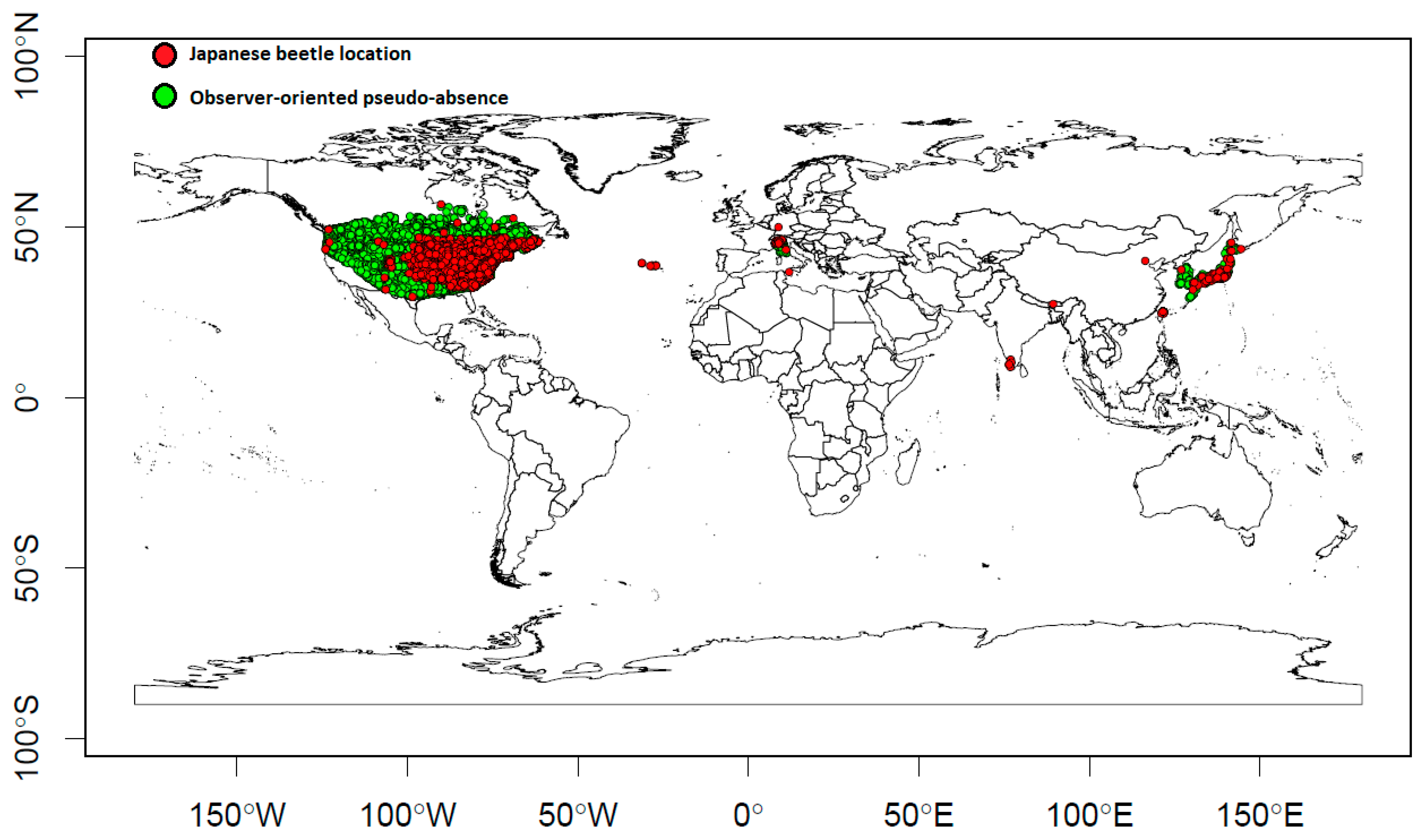
2.1. Presences and Observer-Oriented Pseudo-Absences

We considered all occurrences of Pj collected by citizen scientists during the years 2010–2020 around the globe, extracted from the iNaturalist platform [19]. We downloaded this data using the ‘get_inat_obs’ function in the R package ‘rinat’ [20]. We only considered species locations (with geographic coordinates) collected between June and September, as this corresponds to the active biological period of our target species [21]. iNaturalist is a citizen science-based, open-access platform aimed at recording biodiversity worldwide, and it allows for the easy downloading of species occurrences using specific queries (i.e., place, date, taxon, observer, etc.).
Similar to [14], to select pseudo-absences we listed all the observers of Pj, and then downloaded, from iNaturalist, all the occurrences of all the species (i.e., including both plants and animals, but excluding those of Pj) collected by those observers. We downloaded this data using the ‘get_inat_obs_user’ function in the R package ‘rinat’ [20]. Similar to species’ occurrences, we only considered observer-oriented (oo-) pseudo-absences collected during the years 2010–2020, also between June and September, with geographic coordinates. Thus, in order to avoid introducing false pseudo-absences in which the target species had not yet colonized the area, we applied two spatial filters: (1) we limited oo-pseudo-absences to countries in which the Pj was observed (Table S1); and (2) to those occurring inside the minimum convex polygons (shown in Figure S1, derived using the function ‘mcp’ in the R package ‘adehabitatHR’) [22] estimated around our target species locations, after spatial clustering was carried out using the ‘Mclust’ function in the R package ‘mclust’ [23].

2.2. Predictor Variables

For the current period (2010–2020), we considered an initial number of 34 predictors (2 topographic, 10 land cover, 19 bioclimatic, and 3 anthropogenic variables) to represent the habitat characteristics of Pj [7] (Table 1).
We derived topographic variables from ASTER GDEM [24] available at a spatial resolution of 15 m), while land cover features were derived from the recent European Space Agency Climate Change Initiative Land Cover layers (ESA-CCI 2019, with a spatial resolution of 300 m) [25]. This database provides yearly spatial data for the period 1992–2019, at a spatial resolution of 300 m. We used data from the period 2010–2019, as it best matched the data of our target species. Relating temporally mismatching species locations and predictors could lead to a biased estimation, due to the annual variation in the climatic and land-use conditions [26]. We grouped the initial 21 classes available in the ESA CCI dataset into 10 land cover types (including percentage of human settlements, see below), and from these derived the Shannon habitat diversity index (Table 1). Moreover, we considered 19 bioclimatic predictors derived from the WorldClim2 dataset [27] for the current period (2010–2018 average), at a 2.5 min resolution (≈5 km). Finally, we included the anthropogenic variables encompassed percentages (see above) of human settlements, human population density, available at the spatial resolution of 1 km [28] (averaging the values of the years 2010–2020), and the distance to airports derived from [29,30]. All these predictors were resampled at a spatial resolution of 5 km.
Thus, we estimated the variance inflation factor (VIF) [31], considering all values of the predictors around the globe (not only at the occurrence of the Japanese beetle) to avoid the negative effect of multicollinearity among predictors on SDMs. In detail, we carried out a stepwise procedure that removed predictors until the highest VIF value was <3 [31].
For the year 2050, we considered as constant the two topographic predictors used for the current period, but estimated future land cover based on a recent dataset developed by Clark labs for ESRI (land cover projection 2050, at a spatial resolution of 300 m [32]. This dataset, derived from the ESA CCI dataset mentioned above, provided spatial information of land cover types (the same considered for the current period) from which we also derived the Shannon habitat diversity index for the year 2050 (Table 1). To the best of our knowledge, this is the first time such a high-resolution land cover dataset, available for a global scale for the period 2050, was used to forecast species distribution. Moreover, we considered the same 19 bioclimatic predictors collected for the current period, but estimated for the year 2050 at 2.5 min resolution (≈5 km). These were derived from future climate change scenarios available for the period 2040–2060 [33]. Similar to [34,35], to reduce single GCM uncertainty [36,37], we also considered four climate change scenarios derived from eight general circulation models (GCMs: BCC-CSM2-MR, CNRM-CM6-1, CNRM-ESM2-1, CanESM5, IPSL-CM6A-LR, MIROC-ES2L, MIROC6, and MRI-ESM2-0), representing four widely used representative concentration pathways (RCP 2.6, RCP 4.5, RCP 7, and RCP 8.5) for 2050. These scenarios derived from the sixth assessment of the Intergovernmental Panel for Climate Change [38]. The selected RCPs represent four possible greenhouse gas emission trajectories, ranging from low (RCP 2.6) to high (RCP 8.5), corresponding to increases in global radiative forcing [34]. Specifically, the increase of the global mean surface temperature in 2050 is likely to be ≈1.67 °C under RCP 2.6, ≈1.99 °C under RCP 4.5, ≈2.18 °C under RCP 7, and ≈2.42 °C under RCP8.5 [39]. The anthropogenic variables encompassed percentages of human settlements (derived from land cover projection 2050) and human population density for the year 2050 were extracted from the SEDAC 2000–2100 1-km grid dataset (see above). Similar to the two topographic predictors, we considered distance to airports as constant, as there are currently no projections for the future distribution of airports for the year 2050. All these predictors were resampled at a spatial resolution of 5 km.
Similar to the current period, for the year 2050 we calculated VIF (Table 1) for each of the RCP scenarios considered.

2.3. Species Distribution Models in INLA

To estimate Pj distribution on a global scale, we combined presence and oo-pseudo-absence locations with predictor variables for the current period, using the recently developed method of integrated nested Laplace approximation (INLA) [40]. Compared to other existing Bayesian methods (i.e., the Monte Carlo Markov chain), INLA has several benefits. For example, (i) INLA provides robust and accurate results [41], (ii) is extremely fast compared to other existing frequentist and Bayesian modelling approaches (especially in light of the growing availability of big datasets) [42], and (iii) is one of the very few modelling frameworks that explicitly accounts for spatial autocorrelation among species locations (i.e., dependency among species locations) [43], by incorporating spatial random effects into binomial models (effective in producing SDM-type spatial predictions) [44].
We specifically developed a binomial model in INLA, considering Pj presence/oo-pseudo-absence as the response variable, with uncorrelated predictor variables as the fixed effect, and we also took into account spatial dependency among species locations using the stochastic partial differential equation (SPDE) approach [45], based on computations using a Gaussian Markov random field representation of the Gaussian field [42].
To avoid a huge number of oo-pseudo-absences bias in the results, we considered the same number of species occurrences to serve as oo-pseudo-absences (see Results section below). We repeated this procedure 10 times and found consistent results for the further analyses. We specified that we did not select a total of 10,000 pseudo-absences (often considered in SDMs) [46] as the number of Pj occurrences exceeded this number (see Results section below).
We tested the predictive accuracy of our model using 10-fold cross-validations, splitting our initial dataset in two random groups, one to train the model, with ≈90% of the locations, and the second to validate them, with ≈10% of the locations [47]. We specifically considered two validation statistics: (i) the area under the receiver operating characteristic curve (AUC), and (ii) the true skills statistic (TSS). The former ranged between 0 and 1 (worse than a random model and best discriminating model, respectively) while the latter ranged between −1 and 1 (higher values indicate a good predictive accuracy, while 0 indicates random prediction).
Assuming that the current occurrence of Pj adequately reflects the habitat requirements of this pest species, we projected its occurrence around the globe, according to the future environmental and anthropogenic conditions of the year 2050. Thus, we converted the resulting continuous maps of current and future distribution into binary models, considering threshold values estimated by maximizing TSS [48,49]. Values higher or lower than this threshold represented sites where Pj is likely to occur or not occur, respectively.

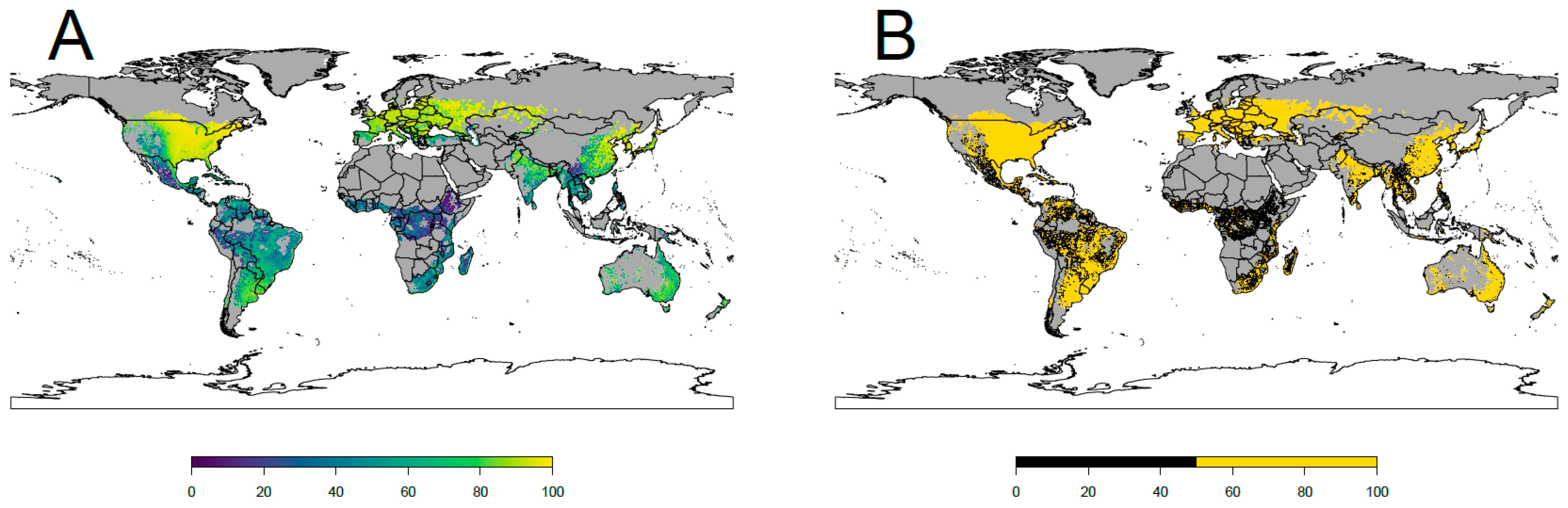
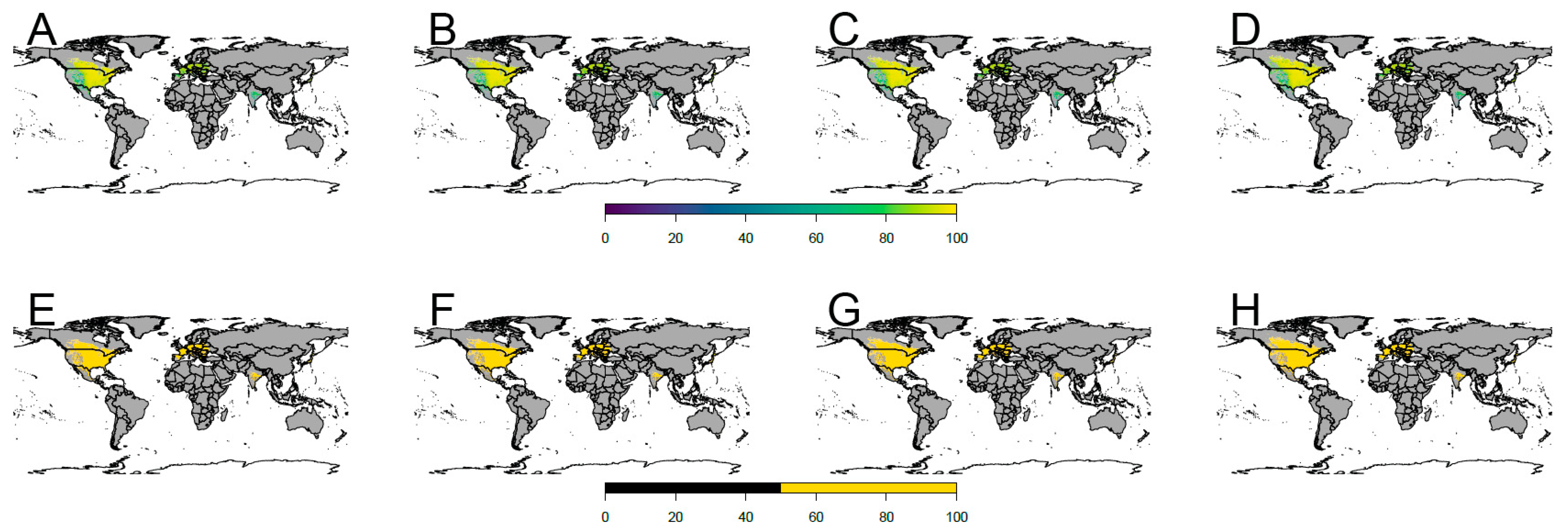
2.4. Definition of the Areas Suitable for the Colonization of the Japanese Beetle
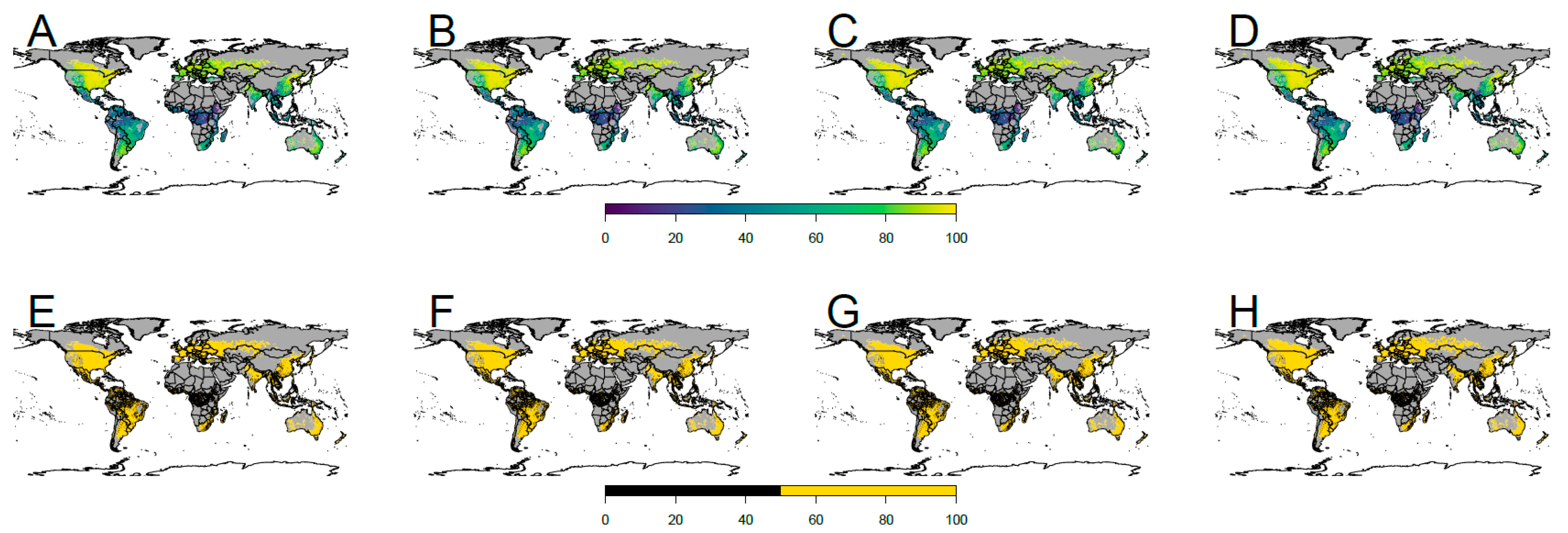
SDMs carried out for very large geographic areas do not always completely capture all the details in species distributions, and could potentially project some false presences beyond the actual species ranges [50]. Thus, we combined Pj occurrences with the resulting non-multi-correlated predictors for the current situation, to identify novel environments in which predictions based on SDMs were uncertain and were not considered for extrapolations. Similar to [12], instead of using the multivariate environmental similarity surface (MESS) [51], we used a modified version of MESS (mMESS) [52]. We estimated using the mMESS model, instead of MESS, as the former does not rely on the use of the most dissimilar variable as an indicator of overall similarity, but rather considers all predictors [52]. In mMESS, values equal to or higher than one indicate that a pixel has at least one predictor variable with values outside the range of the species locations, and thus, it should not be considered for the extrapolations of SDMs [52].
Moreover, since the sum of degree days the beetle needs to complete its development from larva into an adult is a strong limiting factor for the distribution of our target species [21,53], we derived a global map of degree days (DD) from the WorldClim2 monthly dataset. As Pj need a minimum of 711 DD, with a soil temperature greater than 10 °C, to complete its life cycle [21,54] we estimated DD as the sum of all monthly temperatures greater than 10 °C, multiplied by the total number of days using the function ‘growingDegDays’ in the R package ‘envirem’ [55]. Then, based on [54], we considered only areas with a minimum number of degree days above 711.
Similar to the current period, for the year 2050 we calculated mMESS and DD for each of the RCP scenarios considered. Moreover, similar to [35,56], we identified suitable areas accessible to Pj in the future by multiplying the yearly dispersal distance of 59.463 km/year, derived from 1321.4 m/day [57] × 45 days of life/year [58], for the total number of years (n = 30, from 2020 to 2050). The resulting distances were divided by the number of years larvae would take to develop in the adult stage (711 < DD < 1422 two years, DD > 1422 one year) [21], and then used to define accessible areas around current occurrences.

3. Results

Using the data available in iNaturalist between June and September in the years 2010–2020, we collected a total of 24,721 occurrences of Pj, uploaded by a total of 14,911 observers who also collected a total of 892,121 non-target species occurrences (Figure 1), which we initially considered as oo-pseudo-absences. Thus, our dataset consisted of 11,204 cells (at 5 × 5 km2 resolution) in which Pj occurred, and a total of 33,376 cells in which the same observers of our target species collected occurrences of species other than our target species (after applying spatial filters related to countries and minimum convex polygon around Pj occurrences).
Considering both current (2010–2020) and future scenarios (2050), we found 18 predictors with VIF values >3 (multi-correlated: Table 1), and thus, we considered the remaining 16 predictors in the further analyses.
Among the 16 predictors used in the analysis, we found that in 2050, those linked to natural and semi-natural habitats increase, while those linked to water and to human activity decrease (Table S2). This trend is similar in all continents with two exceptions, Africa and Australia, with increasing urban areas and sparse vegetation, respectively (Table S2).
We found that Pj is significantly and positively related to the percentage of croplands, annual temperature range, habitat diversity, percentage of human settlements, and human population density; it is negatively related to the distance to airports, elevation, mean temperature diurnal range, wetlands, and waters (Table 2).
Ten-fold cross-validations showed the high predictive accuracy of our INLA SPDE model, with the values of AUC and TSS equal to 0.921 ± 0.028 and 0.914 ± 0.037, respectively.
Considering the current conditions, we estimated that 47,970,200 km2 are potentially suitable for Pj around the globe (Table 3; Figure 2). This value included the 6,097,741 km2 already occupied by the species, and corresponded to the 12.71% of the total suitable areas available. Among the non-native territories, the United States and Canada (North America) are those most affected by Pj, with around 50% of the suitable areas already occupied.
Considering future conditions, we found that Pj occurrence increases in 2050. Indeed, according to land-use and climatic change scenarios, suitable areas for Pj would account for between 53,418,200 km2 and 59,126,825 km2 of the globe (Table 4; Figure 3). Most of the suitable territories are in North America and increase according to the increase in temperature, while in Central and South America there are fewer suitable areas available in the future, but their expansion remains constant while temperature increases (Table 4).
However, these areas dramatically decrease when Pj dispersal abilities are included in our predictions: 21,404,500 km2 according to the RCP 2.6, 22,596,300 km2 according to the RCP 4.5, 22,969,900 km2 according to the RCP 7, and 24,029,275 km2 according to the RCP 8.5 (Table 4; Figure 4).

4. Discussion

Our results highlight the current distribution and the future worldwide expansion of the invasive destructive pest Pj as a consequence of both climate and land-use change. Due to its strong adaptability, and its highly polyphagous behavior once outside its range, this species has expanded very rapidly, firstly in North America and secondly in Europe, becoming a more serious pest than in its area of origin [54,59,60]. From our models, it emerges that the species will rapidly expand its distribution range in the future, especially because of the general increase in annual temperatures, which both favor the species reproduction, and increase the surface of suitable areas [61]. The future changes in land use seemed not to have a crucial effect in the spread of Pj.

4.1. Current Potential Distribution and Effect of Environmental Variables

Based on our results, most of the areas suitable for Pj are not still occupied by the species, especially those located in the Southern Hemisphere. In these areas, Pj has not yet spread [62], although many suitable areas are available. This is most likely due to the asynchrony between the Northern Hemisphere adult activity season (June and July), and the optimal weather conditions for the survival of the adults in the Southern Hemisphere, which is December and January. Therefore, adults that were accidentally transported from the Northern Hemisphere during summer would have found winter conditions in the Southern Hemisphere, with cold temperatures and very few available and edible plants.
North America is the area of the Northern Hemisphere most affected by the species [59]. In particular, in the United States this invasive beetle was accidentally introduced in 1916, and despite management actions to limit its colonization, within the last 100 years it had successfully spread across much of the east of the country [17]. Moreover, according to our results, Pj is extending its range northward into Canada [63], occupying about half of the whole suitable territories of North America. In Europe, Pj was introduced in 2014 and, according to our results, it currently occupies less than 1% of the suitable areas in this continent. However, the aggressiveness of this species, and its rapid spread [57], alarmed European governments, which immediately activated actions to contain the pest and prevent its spread. Currently, Pj is a quarantine pest, designated as a high priority candidate in the new phytosanitary legislation of the European Union [18,64], and is listed in Annex I Part A/1 of Council Directive 2000/29/EC4.
Our results suggest that the areas occupied by the species are those most impacted by anthropogenic activities. In general, human disturbance influences many biological invasions, especially during the earlier stages after introduction [65]. Territories with a high anthropogenic footprint allow the survival of invasive pests in areas with suboptimal (even unsuitable) climate, e.g., via propagule pressure or by the creation of microclimates [66,67]. Indeed, as expected, we found a strong relationship between suitable areas for Pj and their closeness to airports, confirming the crucial role of human-assisted movement in the rapid expansion of this invasive species [68,69,70,71]. In this regard, in Europe the first observations of Pj referred to a small area located in the Ticino Valley Natural Park in Italy, extremely close to Malpensa airport [72].
Human actions, through the modification of landscapes and the conversion of natural areas into croplands, favor the spread of pests [73]. Currently, agriculture is a dominant form of land management globally [74], and therefore, it is not surprising that pest species are rapidly expanding. Pj is not an exception. Based on our results, Pj tends to occupy those territories with a large extension of croplands, but also with a high habitat diversity. This beetle is a generalist pest, thriving in large areas of turf and pasture grass for grubs developing [61], feeding with over 300 host plant species in 79 families [15,16,17,18,19,20,21,22,23,24,25,26,27,28,29,30,31,32,33,34,35,36,37,38,39,40,41,42,43,44,45,46,47,48,49,50,51,52,53,54,55,56,57,58,59,60,61,62,63,64,65,66,67,68,69,70,71,72,73,74,75]. Therefore, Pj most likely finds those areas with a greater variety of habitat and plant species, including those of non-economic importance, more suitable to optimize the survival of both grubs and adults. The ability to feed on several hosts also ensures the survival of the species, and explains its ability to adapt to new environments [76,77].
According to already published literature [17,78], among the climatic factors, temperature is the parameter that most influences the expansion of this invasive beetle. Moreover, specific temperature is required for oviposition and larval development [15,53,79]. Thus, our models confirm the role of temperature in affecting the spread of Pj, and show that areas with high annual temperatures, and low daily temperature fluctuations, are highly suitable for the beetles. Consequently, we can also include areas with temperate (maritime or sub-continental), Mediterranean, and tropical climates in the areas that are suitable for Pj.
Although the role of soil moisture has been recognized as a key parameter to limit the potential spread of Pj [15,80], in our models precipitations have little effect on its distribution. Therefore, based on our climatic projections, we identified suitable areas for the establishment of Pj that also included areas previously considered unsuitable because of the lack of summer rainfall, such as the Mediterranean regions [80]. Soil moisture depends on many factors besides rainfall, such as soil properties [81,82], proximity to water table [83], and the intensity of water consumption by plants [84]. All these aspects are strictly linked to crops productivity [85], and strongly influence the development of Pj grubs [18,86,87]. Therefore, fertile areas, such as the Po Valley (Italy), are certainly more suitable than others for the proliferation of the beetle, regardless of the intensity of atmospheric precipitations.

4.2. Future Potential Distribution

One of the peculiarities of Pj is the ability to undergo a progressive acclimatization to a broad range of environmental conditions and human pressure [7]. In 2050, the new environmental conditions, combined with a rise in temperature between 1.6° and 2.4 °C, will lead to an increase of territories suitable for Pj of up to more than 20% of the current territories. North America is the area with most of the new suitable regions for Pj (up to 59% of the current areas), followed by Asia and Europe. Based on our results, predictor variables such as croplands and human density, positively related to Pj occurrence, decrease in the future, without producing the expected decrease in areas suitable for this species. This is most likely due to the contrasting effects of climate over anthropogenic factors, as already reported in the literature [7]. Indeed, the rise in winter temperature, reducing cold stress especially in areas of the Northern Hemisphere such as Canada and Russia, would change previously unsuitable areas into new climatically suitable ones [17]. Thus, future conditions enable the beetle to complete its life cycle in a single year instead of two [88,89]. This last aspect leads to a considerable increase in the beetle dispersal capacity, with an increase in its ability to colonize new suitable areas in a short time.
Conversely, increasingly hot and dry future conditions reduce the previously suitable range of areas (Petty et al., 2015 [17,90]. However, in contrast to previous studies [17], the narrowing of the suitable range for Pj does not involve all continents in the Southern Hemisphere, but only Central and South America experience a decrease of about 10% of their current suitable territories. In the rest of the Southern Hemisphere, suitable areas increase but only slightly in Australia.
In 2050, even considering the high dispersal capacities of Pj, less than half of its future available areas are reachable. However, our predictions do not take into account future accidental introductions of Pj into new territories (this is not statistically predictable) that could lead to a significant increase in distribution.
Considering that the surface currently occupied by Pj is only 12.71% of the total available, any expansion in the next 30 years is alarming. In North America, Pj would colonize almost all suitable areas, while in Europe it would reach about half of its potential range. In Asia, in the next 30 years, Pj would reach only 10% of the suitable areas. Indeed, in this continent, despite having a suitable surface greater than that of Europe, and almost equivalent to that of North America, large future suitable areas are not accessible to Pj, currently located in the islands (Japanese and Russian), or in sub-optimal areas (Southern India). However, Pj would be able to successfully establish itself in the mainland of Asia, by way of accidental introduction, due to the new climatically favorable habitats outside the distribution of their natural enemies [91].

5. Conclusions

In this study, we identified with great precision the areas that the pest species could reach in the next 30 years. Therefore, we provided useful information to direct all the resources and effort necessary to prevent the introduction and spread of Pj.
However, the distribution and spread of exotic species also depends on a number of factors not considered in our models, such as biotic resistance by native taxa, human aided dispersal, and to a lesser extent, the availability of host plants that limit Pj expansion [7,49], and which have not been well studied or understood. Therefore, we encourage further research, especially aimed at deepening the ecology of the species, and we advocate the further development of new statistical models in which additional biotic factors can be incorporated. Finally, we strongly suggest adopting approaches similar to those used in this study, possibly combining species occurrences collected during standardized sampling on a local scale when available (e.g., in INLA SPDE, including the source of data as a random effect), in order to model invasive species distribution through space and time, and provide ecologically and statistically robust estimates of species occurrence.

Supplementary Materials

The following supporting information can be downloaded at: https://www.mdpi.com/article/10.3390/land11040567/s1, Table S1. List of countries in which the Japanese beetle was observed. Table S2. Proportion of land use variables under current (2010–2020) and future (2050) conditions (mean ± standard deviation). Difference between mean future and current conditions is also shown: Figure S1. Figure S1: minimum convex polygons, delimited with black lines and corresponding surfaces above sea level in red, estimated around locations of the Japanese beetle.

Author Contributions

Conceptualization, F.D.R. and P.M.; methodology, F.D.R. and P.M.; software, F.D.R. and P.M.; validation, F.D.R. and P.M.; formal analysis, F.D.R. and P.M.; investigation, F.D.R. and P.M.; data curation, F.D.R. and P.M.; writing—original draft preparation, F.D.R. and P.M.; writing—review and editing, F.D.R. and P.M. All authors have read and agreed to the published version of the manuscript.

Funding

This research received no external funding.

Institutional Review Board Statement

Not applicable.

Informed Consent Statement

Not applicable.

Data Availability Statement

Acknowledgments

We thank all citizen scientists that uploaded their observations on iNaturalist (for this and the next generations), and the R-INLA team for developing robust and open access tools for statistical analyses. We also thank the European Space Agency Climate Change Initiative for making yearly spatial land cover data freely available, worldclim2 developers, SEDAC for the free spatial population data and projections, and Clark Labs and ESRI for making the land cover projection 2050 freely available.

Conflicts of Interest

The authors declare no conflict of interest.

References

  1. Seebens, H.; Blackburn, T.M.; Dyer, E.E.; Genovesi, P.; Hulme, P.E.; Jeschke, J.M.; Pagad, S.; Pyšek, P.; Winter, M.; Arianoutsou, M.; et al. No saturation in the accumulation of alien species worldwide. Nat. Commun. 2017, 8, 14435. [Google Scholar] [CrossRef] [PubMed]
  2. Bellard, C.; Cassey, P.; Blackburn, T.M. Alien species as a driver of recent extinctions. Biol. Lett. 2016, 12, 20150623. [Google Scholar] [CrossRef] [PubMed]
  3. Bradshaw, C.J.A.; Leroy, B.; Bellard, C.; Roiz, D.; Albert, C.; Fournier, A.; Barbet-Massin, M.; Salles, J.-M.; Simard, F.; Courchamp, F. Massive yet grossly underestimated global costs of invasive insects. Nat. Commun. 2016, 7, 12986. [Google Scholar] [CrossRef] [PubMed]
  4. Lodge, D.M.; Williams, S.; MacIsaac, H.J.; Hayes, K.R.; Leung BReichard, S.; Mack, R.N.; Moyle, P.B.; Smith, M.; Andow, D.A.; Carlton, J.T. Biological invasions: Recommendations for U.S. policy and management. Ecol. Appl. 2006, 166, 2035–2054. [Google Scholar] [CrossRef] [Green Version]
  5. Hulme, P.E. Trade, transport and trouble: Managing invasive species pathways in an era of globalization. J. Appl. Ecol. 2009, 46, 10–18. [Google Scholar] [CrossRef]
  6. Barbet-Massin, M.; Rome, Q.; Villemant, C.; Courchamp, F. Can species distribution models really predict the expansion of invasive species? PLoS ONE 2018, 13, e0193085. [Google Scholar] [CrossRef] [Green Version]
  7. Zhu, G.; Li, H.; Zhao, L. Incorporating anthropogenic variables into ecological niche modeling to predict areas of invasion of Popillia japonica. J. Pest Sci. 2017, 90, 151–160. [Google Scholar] [CrossRef]
  8. Simberloff, D.; Martin, J.L.; Genovesi, P.; Maris, V.; Wardle, D.A.; Aronson, J.; Courchamp, F.; Galil, B.; García-Berthou, E.; Pascal, M.; et al. Impacts of biological invasions: What’s what and the way forward. Trends Ecol. Evol. 2013, 28, 58–66. [Google Scholar] [CrossRef] [Green Version]
  9. Jeschke, J.M.; Bacher, S.; Blackburn, T.M.; Dick, J.T.A.; Essl, F.; Evans, T.; Gaertner, M.; Hulme, P.E.; Kühn, I.; Mrugała, A.; et al. Defining the Impact of Non-Native Species. Conserv. Biol. 2014, 28, 1188–1194. [Google Scholar] [CrossRef]
  10. Hulme, P.E. Invasion pathways at a crossroad: Policy and research challenges for managing alien species introductions. J. Appl. Ecol. 2015, 52, 1418–1424. [Google Scholar] [CrossRef]
  11. Dyer, E.E.; Cassey, P.; Redding, D.W.; Collen, B.; Franks, V.; Gaston, K.J.; Jones, K.; Kark, S.; Orme, C.D.L.; Blackburn, T.M. The Global Distribution and Drivers of Alien Bird Species Richness. PLoS Biol. 2017, 15, e2000942. [Google Scholar] [CrossRef] [PubMed] [Green Version]
  12. Mori, E.; Menchetti, M.; Zozzoli, R.; Milanesi, P. The importance of taxonomy in species distribution models at a global scale: The case of an overlooked alien squirrel facing taxonomic revision. J. Zool. 2019, 307, 43–52. [Google Scholar] [CrossRef]
  13. Guisan, A.; Tingley, R.; Baumgartner, J.B.; Naujokaitis-Lewis, I.; Sutcliffe, P.R.; Tulloch, A.I.; Regan, T.J.; Brotons, L.; McDonald-Madden, E.; Mantyka-Pringle, C.; et al. Predicting species distributions for conservation decisions. Ecol. Lett. 2013, 16, 1424–1435. [Google Scholar] [CrossRef]
  14. Milanesi, P.; Mori, E.; Menchetti, M. Observer-oriented approach improves species distribution models from citizen science data. Ecol. Evol. 2020, 10, 12104–12114. [Google Scholar] [CrossRef] [PubMed]
  15. Fleming, W.E. Biology of the Japanese Beetle; USDA Technical Bulletin; United States Department of Agriculture: Washington, DC, USA, 1972; Volume 1449, 129p.
  16. United States Department of Agriculture (USDA). Managing the Japanese Beetle: A Homeowner’s Handbook; APHIS 81-25-003; United States Department of Agriculture: Washington, DC, USA, 2015.
  17. Kistner-Thomas, E.J. The Potential Global Distribution and Voltinism of the Japanese Beetle (Coleoptera: Scarabaeidae) Under Current and Future Climates. J. Insect Sci. 2019, 19, 16. [Google Scholar] [CrossRef] [PubMed]
  18. EFSAPlant Health Panel; Bragard, C.; Dehnen-Schmutz, K.; Di Serio, F.; Gonthier, P.; Jacques, M.A.; Jaques Miret, J.A.; Justesen, A.F.; Magnusson, C.S.; Milonas, P.; et al. Scientific Opinion on the pest categorisation of Popillia japonica. EFSA J. 2018, 16, e05438. [Google Scholar]
  19. iNaturalist. Available online: www.inaturalist.org (accessed on 10 February 2022).
  20. Barve, V.; Hart, E.; Guillou, S. Rinat: Access iNaturalist Data through APIs; R Package Version 0.1.8; R Foundation for Statistical Computing: Vienna, Austria, 2021; Available online: https://CRAN.R-project.org/package=rinat (accessed on 10 February 2022).
  21. Regniere, J.; Rabb, R.L.; Stinner, R.E. Popillia japonica: Simulation of temperature-dependent development of the immatures, and prediction of adult emergence. Environ. Entomol. 1981, 10, 290–296. [Google Scholar] [CrossRef]
  22. Calenge, C.; Fortmann-Roe, S. adehabitatHR: Home Range Estimation; R Package Version 0.4, 19; R Foundation for Statistical Computing: Vienna, Austria, 2021; Available online: https://CRAN.R-project.org/package=adehabitatHR (accessed on 10 February 2022).
  23. Scrucca, L.; Fop, M.; Murphy, T.B.; Raftery, A.E. mclust 5: Clustering, Classification and Density Estimation Using Gaussian Finite Mixture Models. R J. 2016, 8, 289–317. [Google Scholar] [CrossRef] [Green Version]
  24. ASTER GDEM. Available online: https://www.jspacesystems.or.jp/ersdac/GDEM/E/ (accessed on 10 February 2022).
  25. European Space Agency Climate Change Initiative Land Cover Layers. Available online: https://www.esa-landcover-cci.org/?q=node/175 (accessed on 10 February 2022).
  26. Milanesi, P.; Della Rocca, F.; Robinson, R.A. Integrating dynamic environmental predictors and species occurrences: Toward true dynamic species distribution models. Ecol. Evol. 2020, 10, 1087–1092. [Google Scholar] [CrossRef] [Green Version]
  27. Worldclim2 Dataset. Available online: https://www.worldclim.org/data/monthlywth.html (accessed on 10 February 2022).
  28. SEDAC 2000–2100 1-km Grid. Available online: https://sedac.ciesin.columbia.edu/data/set/popdynamics-1-km-downscaled-pop-base-year-projection-ssp-2000-2100-rev01/data-download# (accessed on 10 February 2022).
  29. Map of Airports in the World @ OurAirports. Available online: https://ourairports.com/world.html (accessed on 10 February 2022).
  30. AirLabs Data API. Available online: https://airlabs.co/ (accessed on 10 February 2022).
  31. Zuur, A.F.; Ieno, E.N.; Elphick, C.S. A protocol for data exploration to avoid common statistical problems. Methods Ecol. Evol. 2010, 1, 3–14. [Google Scholar] [CrossRef]
  32. Landcover Projection 2050. Available online: https://www.arcgis.com/home/item.html?id=b5ee7191eda1425fa18c26532683896d (accessed on 10 February 2022).
  33. Worldclim2 Dataset Future Projections. Available online: https://www.worldclim.org/data/cmip6/cmip6_clim2.5m.html (accessed on 10 February 2022).
  34. Ihlow, F.; Courant, J.; Secondi, J.; Herrel, A.; Rebelo, R.; Measey, J.; Lillo, F.; De Villiers, F.A.; Vogt, S.; De Busschere, C.; et al. Impacts of Climate Change on the Global Invasion Potential of the African Clawed Frog Xenopus laevis. PLoS ONE 2016, 11, e0154869. [Google Scholar] [CrossRef] [PubMed] [Green Version]
  35. Della Rocca, F.; Milanesi, P. Combining climate, land use change and dispersal to predict the distribution of endangered species with limited vagility. J. Biogeogr. 2020, 47, 1427–1438. [Google Scholar] [CrossRef]
  36. Pierce, D.W.; Barnett, T.P.; Santer, B.D.; Gleckler, P.J. Selecting global climate models for regional climate change studies. Proc. Natl. Acad. Sci. USA 2009, 106, 8441–8446. [Google Scholar] [CrossRef] [Green Version]
  37. Her, Y.; Yoo, S.-H.; Cho, J.; Hwang, S.; Jeong, J.; Seong, C. Uncertainty in hydrological analysis of climate change: Multi-parameter vs. multi-GCM ensemble predictions. Sci. Rep. 2019, 9, 4974. [Google Scholar] [CrossRef] [Green Version]
  38. CMIP Phase 6—CMIP6. Available online: https://www.wcrp-climate.org/wgcm-cmip/wgcm-cmip6 (accessed on 10 February 2022).
  39. Sung, H.M.; Kim, J.; Shim, S.; Seo, J.-B.; Kwon, S.-H.; Sun, M.-A.; Moon, H.; Lee, J.-H.; Lim, Y.-J.; Boo, K.-O.; et al. Climate Change Projection in the Twenty-First Century Simulated by NIMS-KMA CMIP6 Model Based on New GHGs Concentration Pathways. Asia-Pac. J. Atmos. Sci. 2021, 57, 851–862. [Google Scholar] [CrossRef]
  40. Rue, H.; Martino, S.; Chopin, N. Approximate Bayesian inference for latent Gaussian model by using integrated nested Laplace approximations (with discussion). J. R. Stat. Soc. Ser. B 2009, 71, 319–392. [Google Scholar] [CrossRef]
  41. Engel, M.; Mette, T.; Falk, W. Spatial species distribution models: Using Bayes inference with INLA and SPDE to improve the tree species choice for important European tree species. For. Ecol. Manag. 2022, 507, 119983. [Google Scholar] [CrossRef]
  42. Blangiardo, M.; Cameletti, M.; Baio, G.; Rue, H. Spatial and spatio-temporal models with R-INLA. Spat. Spatio-Temporal Epidemiol. 2013, 4, 33–49. [Google Scholar] [CrossRef] [Green Version]
  43. Martínez-Minaya, J.; Cameletti, M.; Conesa, D.; Pennino, M.G. Species distribution modeling: A statistical review with focus in spatio-temporal issues. Stoch. Hydrol. Hydraul. 2018, 32, 3227–3244. [Google Scholar] [CrossRef]
  44. Beguin, J.; Martino, S.; Rue, H.; Cumming, S.G. Hierarchical analysis of spatially autocorrelated ecological data using integrated nested Laplace approximation. Methods Ecol. Evol. 2012, 3, 921–929. [Google Scholar] [CrossRef]
  45. Lindgren, F.; Rue, H.; Lindström, J. An explicit link between Gaussian fields and Gaussian Markov random fields: The stochastic partial differential equation approach (with discussion). J. R. Stat. Soc. Ser. B 2011, 73, 423–498. [Google Scholar] [CrossRef] [Green Version]
  46. Barbet-Massin, M.; Jiguet, F.; Albert, C.H.; Thuiller, W. Selecting pseudo-absences for species distribution models: How, where and how many? Methods Ecol. Evol. 2012, 3, 327–338. [Google Scholar] [CrossRef]
  47. Thuiller, W.; Lafourcade, B.; Engler, R.; Araújo, M.B. BIOMOD—A platform for ensemble forecasting of species distributions. Ecography 2009, 32, 369–373. [Google Scholar] [CrossRef]
  48. Allouche, O.; Tsoar, A.; Kadmon, R. Assessing the accuracy of species distribution models: Prevalence, kappa and the true skill statistic (TSS). J. Appl. Ecol. 2006, 43, 1223–1232. [Google Scholar] [CrossRef]
  49. Thuiller, W.; Georges, D.; Engler, R.; Breiner, F.; Georges, M.D.; Thuiller, C.W. Package ‘Biomod2’. Species Distribution Modeling within an Ensemble Forecasting Framework. 2016. Available online: https://cran.microsoft.com/snapshot/2016-05-25/web/packages/biomod2/biomod2.pdf (accessed on 10 February 2022).
  50. Keller, V.; Herrando, S.; Voríšek, P.; Franch, M.; Kipson, M.; Milanesi, P.; Martí, D.; Anton, M.; Klvanová, A.; Kalyakin, M.V.; et al. European Breeding Bird Atlas 2: Distribution, Abundance and Change; European Bird Census Council & Lynx Edicions: Barcelona, Spain, 2020. [Google Scholar]
  51. Elith, J.; Kearney, M.; Phillips, S. The art of modelling range-shifting species. Methods Ecol. Evol. 2010, 1, 330–342. [Google Scholar] [CrossRef]
  52. Milanesi, P.; Herrando, S.; Pla, M.; Villero, D.; Keller, V. Towards continental bird distribution models: Environmental variables for the second European breeding bird atlas and identification of priorities for further surveys. Vogelwelt 2017, 137, 53–60. [Google Scholar]
  53. Ludwig, D. The Effects of Temperature on the Development of an Insect (Popillia japonica Newman). Physiol. Zool. 1928, 1, 358–389. [Google Scholar] [CrossRef]
  54. Korycinska, A.; Baker, R.H.A.; Eyre, D. Rapid Pest Risk Analysis (PRA) for: Popillia japonica; Defra: London, UK, 2015; p. 34.
  55. Title, P.O.; Bemmels, J.B. ENVIREM: An expanded set of bioclimatic and topographic variables increases flexibility and improves performance of ecological niche modeling. Ecography 2018, 41, 291–307. [Google Scholar] [CrossRef] [Green Version]
  56. Jaeschke, A.; Bittner, T.; Reineking, B.; Beierkuhnlein, C. Can they keep up with climate change?—Integrating specific dispersal abilities of protected Odonata in species distribution modelling. Insect Conserv. Divers. 2013, 6, 93–103. [Google Scholar] [CrossRef]
  57. Caton, B.P.; Fang, H.; Manoukis, N.C.; Pallipparambil, G.R. Quantifying insect dispersal distances from trapping detections data to predict delimiting survey radii. J. Appl. Entomol. 2021, 146, 203–216. [Google Scholar] [CrossRef]
  58. Klein, M. Popillia japonica (Japanese Beetle); Invasive Species Compendium; CABI: Wallingford, UK, 2008. [Google Scholar]
  59. EPPO. EPPO Global Database. 2022. Available online: https://gd.eppo.int (accessed on 10 February 2022).
  60. CABI. Invasive Species Compendium. CAB International: Wallingford, UK, 2022. Available online: www.cabi.org/isc (accessed on 10 February 2022).
  61. Potter, D.A.; Held, D.W. Biology and Management of the Japanese Beetle. Annu. Rev. Entomol. 2002, 47, 175–205. [Google Scholar] [CrossRef] [PubMed] [Green Version]
  62. Jackson, T.A.; Klein, M.G. Scarabs as Pests: A Continuing Problem. Coleopt. Bull. 2006, 60, 102–119. [Google Scholar] [CrossRef]
  63. CFIA. Popillia japonica (Japanese Beetle); Canadian Food Inspection Agency: Ottawa, ON, Canada, 2020.
  64. EPPO. EPPO Standards: EPPO A1 and A2 Lists of Pests Recommended for Regulation as Quarantine Pests; (PM 1/2(28)); EPPO: Paris, France, 2019. [Google Scholar]
  65. Dietz, H.; Edwards, P.J. Recognition that causal processes change during plant invasion helps explain conflicts in evidence. Ecology 2006, 87, 1359–1367. [Google Scholar] [CrossRef]
  66. Roura-Pascual, N.; Hui, C.; Ikeda, T.; Leday, G.; Richardson, D.M.; Carpintero, S.; Espadaler, X.; Gómez, C.; Guénard, B.; Hartley, S.; et al. Relative roles of climatic suitability and anthropogenic influence in determining the pattern of spread in a global invader. Proc. Natl. Acad. Sci. USA 2011, 108, 220–225. [Google Scholar] [CrossRef] [PubMed] [Green Version]
  67. Beans, C.M.; Kilkenny, F.F.; Galloway, L.F. Climate suitability and human influences combined explain the range expansion of an invasive horticultural plant. Biol. Invasions 2012, 14, 2067–2078. [Google Scholar] [CrossRef] [Green Version]
  68. Liebhold, A.M.; Work, T.T.; McCullough, D.G.; Cavey, J.F. Airline Baggage as a Pathway for Alien Insect Species Invading the United States. Am. Entomol. 2006, 52, 48–54. [Google Scholar] [CrossRef] [Green Version]
  69. Lines, J. Chikungunya in Italy: Globalisation is to blame, not climate change. Br. Med. J. 2007, 335, 576. [Google Scholar] [CrossRef]
  70. McCullough, D.G.; Work, T.T.; Cavey, J.F.; Liebhold, A.M.; Marshall, D. Interceptions of Nonindigenous Plant Pests at US Ports of Entry and Border Crossings Over a 17-year Period. Biol. Invasions 2006, 8, 611–630. [Google Scholar] [CrossRef]
  71. Tatem, A.J.; Hay, S. Climatic similarity and biological exchange in the worldwide airline transportation network. Proc. R. Soc. B Boil. Sci. 2007, 274, 1489–1496. [Google Scholar] [CrossRef] [Green Version]
  72. Pavesi, M.A. Popillia japonica specie aliena invasiva segnalata in Lombardia. L’Informatore Agrar. 2014, 32, 53–55. [Google Scholar]
  73. Bebber, D.P.; Holmes, T.; Gurr, S.J. The global spread of crop pests and pathogens. Glob. Ecol. Biogeogr. 2014, 23, 1398–1407. [Google Scholar] [CrossRef] [Green Version]
  74. Kanianska, R. Agriculture and Its Impact on Land-Use, Environment, and Ecosystem Services. In Landscape Ecology—The Influences of Land Use and Anthropogenic Impacts of Landscape Creation; Almusaed, A., Ed.; IntechOpen: London, UK, 2016. [Google Scholar]
  75. Ladd, T.L. Japanese beetle (Coleoptera: Scarabaeidae): Feeding by adults on minor host and non-host plants. J. Econ. Entomol. 1989, 82, 1616–1619. [Google Scholar] [CrossRef]
  76. Ladd, T.L. Influence of Sugars on the Feeding Response of Japanese Beetles (Coleoptera: Scarabaeidae). J. Econ. Entomol. 1986, 79, 668–671. [Google Scholar] [CrossRef]
  77. Keathley, C.P. Determinants of Host Plant Selection in the Japanese Beetle. Master’s Thesis, University of Kentucky, Lexington, KY, USA, 1998; 128p. [Google Scholar]
  78. Niziolek, O.K.; Berenbaum, M.R.; DeLucia, E.H. Impact of elevated CO2 and increased temperature on Japanese beetle herbivory. Insect Sci. 2013, 20, 513–523. [Google Scholar] [CrossRef] [PubMed]
  79. Allsopp, P.G.; Klein, M.G.; McCoy, E.L. Effect of Soil Moisture and Soil Texture on Oviposition by Japanese Beetle and Rose Chafer (Coleoptera: Scarabaeidae). J. Econ. Entomol. 1992, 85, 2194–2200. [Google Scholar] [CrossRef]
  80. Bourke, P.A. Climatic Aspects of the Possible Establishment of the Japanese Beetle in Europe; Technical Note; World Meteorological Organization: Geneva, Switzerland, 1961; Volume 41, pp. 1–9. [Google Scholar]
  81. Chaney, N.W.; Roundy, J.K.; Herrera–Estrada, J.E.; Wood, E.F. High-resolution modeling of the spatial heterogeneity of soil moisture: Applications in network design. Water Resour. Res. 2015, 51, 619–638. [Google Scholar] [CrossRef] [Green Version]
  82. Fang, X.; Zhao, W.; Wang, L.; Feng, Q.; Ding, J.; Liu, Y.; Zhang, X. Variations of deep soil moisture under different vegetation types and influencing factors in a watershed of the Loess Plateau, China. Hydrol. Earth Syst. Sci. 2016, 20, 3309–3323. [Google Scholar] [CrossRef] [Green Version]
  83. Chen, X.; Hu, Q. Groundwater influences on soil moisture and surface evaporation. J. Hydrol. 2004, 297, 285–300. [Google Scholar] [CrossRef] [Green Version]
  84. Du, S.N.; Bai, G.S.; Liang, Y.L. Effects of soil moisture content and light intensity on the plant growth and leaf physiological characteristics of squash. Chin. J. Appl. Ecol. 2011, 22, 1101–1106. [Google Scholar]
  85. Rossato, L.; Marengo, J.A.; Angelis, C.F.; Pires, L.B.M.; Mendiondo, E.M. Impact of soil moisture over palmer drought severity index and its future projections in Brazil. Braz. J. Water Resour. 2017, 22, 1–16. [Google Scholar] [CrossRef] [Green Version]
  86. Hammond, R.B.; Stinner, B.R. Soybean Foliage Insects in Conservation Tillage Systems: Effects of Tillage, Previous Cropping History, and Soil Insecticide Application. Environ. Entomol. 1987, 16, 524–531. [Google Scholar] [CrossRef]
  87. Shanovich, H.N.; Dean, A.N.; Koch, R.L.; Hodgson, E.W. Biology and Management of Japanese Beetle (Coleoptera: Scarabaeidae) in Corn and Soybean. J. Integr. Pest Manag. 2019, 10, 9. [Google Scholar] [CrossRef]
  88. Bentz, B.J.; Régnière, J.; Fettig, C.J.; Hansen, E.M.; Hayes, J.L.; Hicke, J.A.; Kelsey, R.G.; Negrón, J.F.; Seybold, S.J. Climate Change and Bark Beetles of the Western United States and Canada: Direct and Indirect Effects. BioScience 2010, 60, 602–613. [Google Scholar] [CrossRef]
  89. Everall, N.C.; Johnson, M.F.; Wilby, R.L.; Bennett, C.J. Detecting phenology change in the mayfly Ephemera danica: Responses to spatial and temporal water temperature variations. Ecol. Entomol. 2015, 40, 95–105. [Google Scholar] [CrossRef] [Green Version]
  90. Petty, B.M.; Johnson, D.T.; Steinkraus, D.C. Changes in Abundance of Larvae and Adults ofPopillia japonica (Coleoptera: Scarabaeidae: Rutelinae) and Other White Grub Species in Northwest Arkansas and Their Relation to Regional Temperatures. Fla. Entomol. 2015, 98, 1006–1008. [Google Scholar] [CrossRef] [Green Version]
  91. Furlong, M.J.; Zalucki, M.P. Climate change and biological control: The consequences of increasing temperatures on host–parasitoid interactions. Curr. Opin. Insect Sci. 2017, 20, 39–44. [Google Scholar] [CrossRef] [Green Version]
Figure 1. Study area, the world. Target species locations in red, total observer-oriented pseudo-absences (i.e., observances from locations other than target species, collected by the observers of the target species) in green.
Land 11 00567 g001
Figure 2. Distribution maps of the Japanese beetle, estimated under current conditions derived from INLA SPDE. (A) yellow–blue scale indicates higher–lower occurrence probability values, respectively, (B) areas of predicted species occurrence estimated using a threshold value of 50.3 (threshold values estimated by maximizing TSS), presence shown in orange, while absence shown in black. Areas of uncertain prediction identified by mMESS, and those with DD values below the threshold of 711, are shown in grey.
Land 11 00567 g002
Figure 3. Distribution maps of the Japanese beetle estimated under future conditions (without accounting for species dispersal distance) derived using INLA SPDE. (AD) yellow–blue scale indicates higher–lower occurrence probability values, respectively, (EH) areas of predicted species occurrence estimated using a threshold value of 50.3 (threshold values estimated by maximizing TSS), presence shown in orange, while absence shown in black. Panels (A,E) refer to the future climatic scenario RCP 2.6, (B,F) to RCP 4.5, (C,G) to RCP 7, while (D,H) to RCP 8.5. Areas of uncertain prediction identified by mMESS, and those with DD values below the threshold of 711, are shown in grey.
Land 11 00567 g003
Figure 4. Distribution maps of the Japanese beetle estimated under future conditions (accounting for species dispersal distance) derived from INLA SPDE. (AD) yellow–blue scale indicates higher–lower occurrence probability values, respectively, (EH) areas of predicted species occurrence estimated using a threshold value of 50.3 (threshold values estimated by maximizing TSS), presence shown in orange, while absence shown in black. Panels (A,E) refer to the future climatic scenario RCP 2.6, (B,F) to RCP 4.5, (C,G) to RCP 7, while (D,H) to RCP 8.5. Areas of uncertain prediction identified by mMESS, and those with DD values below the threshold of 711, are shown in grey.
Land 11 00567 g004
Table 1. Predictor variables considered and their relative variance inflation factor (VIF). Predictors with VIF > 3 were not considered in further analysis.
VariableUnit2010–20202050 RCP
2.64.578.5
Altitudem a.s.l.1.7611.6921.6821.6471.703
Slope°1.5481.5371.5061.5071.542
Bare areas%1.9912.0011.8161.7921.854
Deciduous forests%>3>3>3>3>3
Grasslands, scrubs, shrubs%1.5861.6211.6181.5471.611
Needleleaf forests%>3>3>3>3>3
Permanent snow and ice%>3>3>3>3>3
Sparse vegetation%1.3291.3541.3791.3221.385
Waters%1.3641.2561.2441.2091.241
Wetlands%1.1631.1551.1631.1411.145
Croplands%1.6361.4991.4011.4811.428
Shannon habitat diversity indexH′ = −Σ (pi × lnpi)1.2941.3811.3781.3411.378
Human settlements%1.2881.5571.3171.3581.299
Distance to airportsM1.4871.4161.4741.4481.451
Human population densityn/km21.2831.5941.3111.5011.289
Annual mean temperature°C>3>3>3>3>3
Mean diurnal range°C1.8612.1242.2162.0412.176
Isothermality (BIO2/BIO7)°C × 100>3>3>3>3>3
Temperature seasonalityStd. Dev. × 100>3>3>3>3>3
Max temperature of warmest month°C>3>3>3>3>3
Min temperature of coldest month°C>3>3>3>3>3
Temperature annual range°C1.5021.6281.6311.6611.597
Mean temperature of wettest quarter°C>3>3>3>3>3
Mean temperature of driest quarter°C>3>3>3>3>3
Mean temperature of warmest quarter°C>3>3>3>3>3
Mean temperature of coldest quarter°C>3>3>3>3>3
Annual precipitationMm>3>3>3>3>3
Precipitation of wettest monthMm>3>3>3>3>3
Precipitation of driest monthMm1.7421.6651.6741.7241.665
Precipitation seasonalityCoeff. of variation>3>3>3>3>3
Precipitation of wettest quarterMm>3>3>3>3>3
Precipitation of driest quarterMm>3>3>3>3>3
Precipitation of warmest quarterMm1.9762.2052.1982.1492.142
Precipitation of coldest quarterMm>3>3>3>3>3
Table 2. Average coefficients (β) ± standard deviation (S.D.) and significance (*, different from 0) of the predictors considered to model Japanese beetle occurrence in INLA SPDE. Thetas for the spatial random effect, deviance information criterion (DIC), and Watanabe–Akaike information criterion (WAIC) are also shown.
Parameterβ ± S.D.
Intercept−5.971 ± 0.938 *
Altitude−1.001 ± 0.156 *
Bare areas0.065 ± 0.372
Croplands0.928 ± 0.029 *
Distance to airports−3.406 ± 0.423 *
Grasslands, scrubs, and shrubs0.029 ± 0.038
Human population density0.059 ± 0.014 *
Shannon habitat diversity index0.208 ± 0.021 *
Slope−0.081 ± 0.051
Sparse vegetation0.537 ± 1.331
Human settlements0.067 ± 0.006 *
Waters−0.131 ± 0.022 *
Precipitation of driest month0.147 ± 0.101
Precipitation of warmest quarter0.041 ± 0.197
Mean diurnal range−0.451 ± 0.188 *
Temperature annual range1.611 ± 0.537 *
Wetlands−0.254 ± 0.041 *
Theta1−1.091 ± 0.108
Theta2−1.351 ± 0.218
DIC22,936.001
WAIC22,919.409
Table 3. Current distribution and suitable areas (km2) of the Japanese beetle. Data on current distribution were extrapolated by [59] while suitable areas under current conditions were derived by INLA SPDE. Percentage of current distribution on suitable areas is also shown.
Regionkm2Occupied Areas (%)
Current Distribution Suitable Areas
Europe62,181.1010,476,6000.59
Asia (+Russia)416,362.2 (native)11,757,2003.54
North America5,619,197.9011,091,42550.66
Central and South America0.009,376,0500.00
Africa0.001,966,7000.00
Australia0.003,302,2250.00
World6,097,741.2047,970,20012.71
Table 4. Future distribution (km2) of the Japanese beetle. Suitable and reachable (from the territory currently occupied) areas were estimated alternatively, excluding and accounting for the dispersal ability of the species. Percentage of reachable suitable areas is also shown.
RegionRCP 2.6RCP 4.5RCP 7.0RCP 8.5
Suitable Areas (km2)Europe11,154,57511,911,97512,305,17512,595,200
Asia (+Russia)13,133,02513,828,02514,240,10014,543,875
North America14,938,80016,131,27516,539,05017,640,250
Central and South America8,412,6758,480,3258,460,5258,525,250
Africa2,346,1252,342,2752,397,4002,385,500
Australia3,433,0003,432,0753,448,4253,436,750
World53,418,20056,125,95057,390,67559,126,825
Reachable areas (km2)Europe5,638,7755,724,3505,749,1755,774,200
Asia (+Russia)1,377,8251,373,4001,377,1501,376,525
North America14,387,90015,498,55015,843,57516,878,550
Central and South America0000
Africa0000
Australia0000
World21,404,50022,596,30022,969,90024,029,275
Occupied areas (%)Europe50.5548.0646.7245.84
Asia (+Russia)10.499.939.679.46
North America96.3196.0895.7995.68
Central and South America0.000.000.000.00
Africa0.000.000.000.00
Australia0.000.000.000.00
World40.0740.2640.0240.64
Publisher’s Note: MDPI stays neutral with regard to jurisdictional claims in published maps and institutional affiliations.

