Article

Half-Century of Forest Change in a Neotropical Peri-Urban Landscape: Drivers and Trends

by
Juan Von Thaden
1,
Gilberto Binnqüist-Cervantes
2,
Octavio Pérez-Maqueo
3 and
Debora Lithgow
3,*
1
Instituto de Estudios Ambientales, Universidad de la Sierra Juárez, Avenida Universidad s/n, Ixtlán de Juárez, Oaxaca 68725, Mexico
2
Laboratorio de Planeación Ambiental, Departamento El hombre y su Ambiente, UAM-Xochimilco, Calzada del Hueso 1100, Coyoacan, Mexico City 04960, Mexico
3
Red de Ambiente y Sustentabilidad, Instituto de Ecología, A.C., Carretera antigua a Coatepec 351, Xalapa, Veracruz 91073, Mexico
*
Author to whom correspondence should be addressed.
Land 2022, 11(4), 522; https://doi.org/10.3390/land11040522
Submission received: 28 February 2022 / Revised: 31 March 2022 / Accepted: 1 April 2022 / Published: 4 April 2022
(This article belongs to the Special Issue Ecosystem Services and Biodiversity of Peri-Urban Landscapes)

Abstract

:
Neotropical forested landscapes have become agricultural areas and human settlements, causing forest fragmentation, land degradation, and habitat loss. Nonetheless, complex tree cover loss and recovery processes may occur even while urban areas expand. Biophysical, social, political, and economic drivers influence forest loss or recovery over time. This study analyzes land-use change dynamics in urban and peri-urban landscapes in the western sector of Xalapa City between 1966–2018 and identifies the primary drivers that have played a significant role in deforestation and forest recovery processes. The main finding denotes the city’s expansion between 1966 and 2018, initially covering 8% of the study area and increasing to 27%. However, between 1966 and 2018, 15% of forest cover was lost in net terms, a finding ascribed to forest recovery in some abandoned areas. Social and biophysical variables significantly influenced deforestation and forest recovery trends, and few variables were singular to one process. The deceleration of forest loss and accomplishing tree cover recovery are possible in some urban settings. In this context, green urban and peri-urban landscapes become strategic to achieve more sustainable cities. Among other benefits, green areas provide landscape connectivity, temperature regulation, air quality improvement, noise dampening, and recreational areas.

1. Introduction

Globally, forests cover 31% of our planet’s land surface, but more than half of these forests show some degree of perturbation, and half of the tropical forests have gotten lost during the past half-century [1]. The most significant threats to forests worldwide are deforestation; forest replacement for other land uses (such as agriculture and urban development); and degradation of forest health, structural integrity, and resilience. Forest loss and degradation are global concerns considering how these processes threaten the survival of 80% of terrestrial biodiversity and the supplies of a wide range of benefits essential to human well-being; these benefits are known as “ecosystem services” (ES; [2]).
The high concentration of ES beneficiaries in cities and the scarce urban green areas highlight the importance of urban and peri-urban forests [2,3] that directly influence the provision of key ES, such as improvement of air quality, water and temperature regulation, noise reduction, and sites of recreation [4,5,6].In this sense, assessing the dynamics of forest cover allows an indirect evaluation of the provision and regulation of crucial ES to the well-being of the inhabitants of cities.
According to the IUCN [3], the livelihood of 1.6 billion people is directly dependent on forest services such as timber, food, medicine, clean water, and cultural values [4]. Moreover, other than to communities entirely forest-dependent, these ecosystems also provide services at regional and global scales. For example, forests prevent soil erosion, loss of productivity, downstream sedimentation, and eutrophication [5]. The loss of services implies that deforestation threatens world food security [6,7] and water security in some of the world’s most populated areas. The vital contribution of forest services to cities was recognized two decades ago when a meta-analysis revealed that one-third of the world’s largest cities are dependent on these ecosystems for their drinking water [8]. At the same time, deforestation is the second-largest source of global CO2 emissions, transforming forests from a carbon sink to a source. In response, scientists worldwide have highlighted the importance of forest climate regulation and carbon sequestration services as cornerstones in the global efforts to tackle climate change. These efforts include a wide array of strategies intended to meet climate stabilization targets by 2030, ranging from forest conservation and restoration efforts to recovering and creating green urban and peri-urban landscapes [9].
Despite the internationally recognized importance of healthy forests to human well-being, direct and indirect drivers of change have increased their impact at a landscape scale in the last 50 years. The indirect drivers include increased consumption patterns, such as the demand for raised meat, soy, and palm oil [10]. In turn, direct drivers of forest loss and degradation include climate change, invasive species, and changes in land use and land cover (i.e., LULC). LULC remains the most critical cause of degradation in all terrestrial ecosystems worldwide, as the global rate of deforestation between 2015 and 2020 amounted to 10 million hectares per year [1]. Urban areas play a crucial role in deforestation trends in this setting, and most studies show a positive correlation between forest loss and urban growth [11]. However, not all cities grow evenly at the same rate or are driven by the same socioeconomic factors. Better management of urban and peri-urban sprawl patterns and the recovery of green urban and peri-urban landscapes could promote a shift in forest degradation trends.
The United Nations Decade of Ecosystem Restoration 2021–2030 initiative (i.e., the Decade) is a global call for action to scale up efforts to reduce ecosystem degradation trends and reverse the associated harm to human well-being. Among the strategies promoted by the UN Decade initiative are assessing and monitoring the temporal trends of ecosystem degradation triggering drivers to produce informed conservation and restoration strategies, including greener cities and forest landscape recovery in peri-urban landscapes [12].
There is no doubt that contemporary landscapes emerged from very long-term dynamics [13]. However, the variables that configured those landscapes vary within and between regions [14]. Consequently, analyzing the variables most strongly associated with forest loss–forest recovery dynamics, quantifying the rates and trends of change, and identifying the affected areas are essential tasks for sound decision making on sustainable forest use and prioritizing interventions in highly populated areas. Additionally, the conservation of biodiversity and critical ES for human welfare requires scientific information [15].
A driver is any factor that alters some aspect of an ecosystem [16]; there are two types: direct or indirect. A direct driver influences ecosystem processes and can be biophysical (earthquakes, volcano eruptions, plagues, and floods, among others). An indirect driver operates more diffusely, generally altering one or more direct drivers (e.g., floods, landslides, etc.). Furthermore, its influence is determined by understanding what its effects are on a direct driver, which includes topics such as demography (population dynamics aand migration patterns, amongst others), economy (consumption patterns, production, and more), policies (conservation programs and agriculture development programs, among others), and cultural/religious aspects.
The analysis and design of better management strategies in urban and peri-urban forests are urgent tasks, because world urban populations will increase to nearly 5 billion by 2030 [17], requiring more goods and services. Simultaneously, urban growth would impact the provision of those services, independently of each population center’s growth dynamic, which will be determined by its particular biophysical, environmental, political, and economic features [11].
According to most deforestation studies, socioeconomic factors have a weaker, nonlinear, or less direct relationship with this process than biophysical variables [18,19,20]. Similarly, forest recovery studies suggest that biophysical variables, such as climate, elevation, soil, and slope, tend to be associated with the probability and speed of forest regrowth [21,22,23,24]. However, these biophysical factors are difficult to control by policy [25], but this should not encourage non-action strategies. The high biodiversity and sprawl dynamics in Latin America could serve to identify opportunities for action.
As in other countries, urban development has occurred in Mexico at the expense of forest loss and fragmentation of green and agricultural areas in peri-urban “semi-rural” territories. One of the main drivers leading to urban sprawl in intermediate cities and semiurban areas is rapid population growth [26]. In Mexico, the population boom and the outsourcing of the urban economy are intertwined, turning cities into magnets for the rural population that needs to satisfy housing needs [27]. Moreover, the reforms to the Mexican Constitution allowing individual possession and sale of ejidal and communal lands triggered three responses that have contributed to the situation as mentioned above [28]. First, some farming centers sold their rural lands at a “bargain” price to real estate developers that constructed residential units in territorially inadequate and disconnected sites [28]. Second, socio-political activist organizations promoted irregular settlements, taking advantage of vulnerable communities. Third, the new residential areas were conceived for high-income segments of the population interested in living surrounded by natural vegetation with the comforts of urban areas.
This study proposes understanding the forest loss and gaining processes during the last half-century in Xalapa through a LULC analysis and the possible biophysical and socioeconomic drivers. A series of land use and vegetation cover maps, prepared for the years between 1966 and 2018, helped identify biophysical and socioeconomic variables which, based on the literature, are significant drivers for deforestation and forest recovery processes worldwide. Finally, the possible alternatives to increase the resilience of Xalapa city through forest restoration and the recovery of green areas in urban and peri-urban landscapes are discussed.

2. Materials and Methods
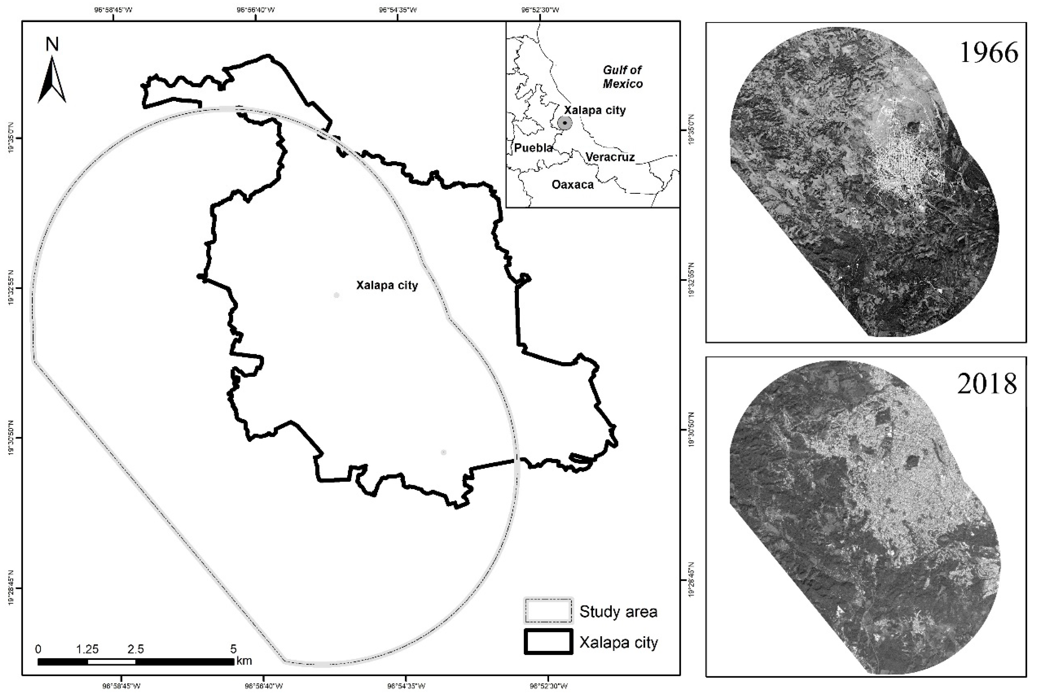
2.1. Study Area

Like the rest of the world, the most significant force causing the loss of ecosystems and their biodiversity in Mexico is deforestation. According to Sánchez et al., 2009, natural communities extended across 72.5% of the country in 2002, but only 70% of these were relatively undisturbed. Most of this degradation took place before the 1970s; by 2002, there would have been a net loss of up to 103,289 km2 of humid tropical forests, 94,223 km2 of sub-humid forests, 129,000 km2 of temperate forests, 91,000 km2 of xerophilous scrub, and more than 59,000 km2 of grasslands. This loss has important implications for worldwide biodiversity conservation, as Mexico is one of 15 megadiverse countries that concentrate between 60 and 70% of global biodiversity [29,30].
The Trans-Mexican Volcanic Belt (TVB) embodies a significant region in the country. As a complex set of volcanic mountains, it extends across the territory from west to east, from Cabo Corrientes, in Nayarit, to the Sierra Chinconquiaco, in Veracruz (21°38′24″ N, 18°23′24″ S, 96°22′12″ E, and 105°45′00″ W), varying in elevation between 1500 and 5600 masl [31]. The geological and climatic history, topographic heterogeneity, and species distribution have served to recognize the TVB as a biogeographic transition zone and a center of diversification and the endemism for a great variety of taxa [32].
During the past centuries, human influence on the TVB modified the high mountain landscapes, with crops and pastures for livestock replacing the natural vegetation [33]. Such is the case for Veracruz, the state with the second-highest deforestation rate in Mexico, with roughly 75% of its territory having been clear cut [34]. The dominant vegetation types consist of conifer and oak forests, humid montane forests, moist (broadleaf) and dry (tropical deciduous) forests, and grasslands, including various wetlands. Agriculture incorporates 75% of the state’s surface, with a large proportion dedicated to sown pastures for livestock raising, an activity of great economic importance within the state [34].
This study was performed in the western sector of the city of Xalapa, the capital of the state of Veracruz, covering 12,066 ha, with 496,627 inhabitants and located in east-central Mexico (Figure 1). Xalapa transitioned in 400 years from a colonial city organized according to a Hispanic urban graticule (a regular orthogonal grid system) to an irregular system. Xalapa’s characteristic streets and city blocks emerged despite the verdant landscape, without adhering to the urban development plan or any other land use planning instrument [35]. With significant numbers of irregular human settlements, Xalapa’s urban growth escalated deforestation rates, water pollution by sanitary discharges, and risk from landslides [36,37]. Notwithstanding, Xalapa retains 12.16 m2 of green area per inhabitant, an acceptable ratio according to the World Health Organization, which recommends between 10 and 15 m2. The proportion of green areas in Xalapa allows for the improvement of the city’s resilience through forest restoration and green areas rehabilitation. However, the first step is to confront, strategically and responsibly, the accelerated land-use change that triggers the sprawl of formal and informal urbanization [29]. Improving Xalapa city’s growth depends on understanding the economic, demographic, and sociocultural dynamics that defined the regional landscape. This type of analysis also is needed to understand which socioeconomic or biophysical variables better explain deforestation or forest recovery patterns in different regions and thus encourage more effective regional conservation and restoration strategies [20].
This mountainous and biodiverse city includes a broad range of elevations (i.e., 1120–1720 m.a.s.l.); given this elevation gradient, the climate fluctuates between humid temperate and humid semi-temperate [38]. The predominant vegetation is essentially tropical montane cloud forest, combined with oak forest, coniferous forest, tropical dry forest, and riparian vegetation [38]. An uneven topography contributes to Xalapa’s broad range of elevations (i.e., 850–2125 m.a.s.l.; [39]). From a technical point of view, the study area was delimited because of the availability of half a century of imagery.

2.2. Land Use and Land Cover Maps (LULC)

The satellite imagery and aerial photos used to generate LULC maps were obtained from the following sources: CORONA satellite imagery of 1966 (9-m spatial resolution) downloaded from the USGS (http://glovis.usgs.gov/; accessed on 18 February 2020). Aerial photos from 1980 (2-m spatial resolution) and 1995 (2-m spatial resolution) were downloaded from INEGI. Satellite Images from 2008 (2.5-m spatial resolution) and 2018 (30-cm spatial resolution) were obtained from the Mexican Navy (Ermex: http://ermexnuevageneracion.blogspot.mx/p/contacto.html; accessed on 27 June 2016) and NextView Digital Glove, respectively. Topographic illumination, normalization, and atmospheric corrections were performed on all images. Image classification was performed using Trimble eCognition® Developer 9.0, with an object-based approach and the random forest (RF) classifier (Random Trees in eCognition). Two LULC categories were identified in this study, consisting of forested and non-forested sites. Following the recommendations of Campbell [40], an average of 50 sample units per land-use type of reference data (100 in total) that originated from field visits to plots, with a minimum of 60 × 60 m of homogeneous vegetation (August 2013 to March 2014 and June–August 2020), were used to train the classification. Considering that these sampling units may not reflect LULC before the dates, they were re-interpreted and adjusted by visually inspecting images from each previous period successively, as Campbell [40] described. This amount of training data is considered more than sufficient to train the RF classifier accurately for these two categories. To validate the final maps, 100 reference sample units, independent of those selected for image classification, were used to generate an area-based error matrix and a Kappa index for each classification [41].

2.3. Analysis of Forest Cover Change

A cartographic overlap assessment served to calculate the magnitude and tendencies of forest cover change and by estimating differences in forest cover between periods (1966–1980; 1980–1995; 1995–2008; 2008–2018). Annual deforestation rates for closed and open forest (r) were calculated using the compound interest-rate formula [42]:
r = 1/(t2 − t1) ln A2/A1
where A1 = forest area at t1 (initial area), and A2 = forest area at t2 (final area).

2.4. Potential Drivers of Forest Change

A logistic regression model was used to identify possible drivers of forest change (deforestation or forest recovery) in our study area [43]. Our maps, derived from Landsat imagery, were used to identify areas with forest cover losses (deforestation) or gains (forest recovery) versus areas of no change [44] for the periods of 1966–1980, 1980–1995, 1995–2008, and 2008–2018. Additionally, a transition map of deforestation and another of forest recovery was prepared for each period. In each of the transition maps, the areas of deforestation and forest recovery were detected to obtain their centroids (points). Then, 500 points were randomly selected with a minimum separation of 250 m to avoid spatial autocorrelation; the centroids’ independence was verified with Moran’s I coefficient.
Those random points served to extract data from layers of 12 biophysical and socioeconomic variables considered as possible predictors for both deforestation and forest recovery during the study period (Table 1). The availability of information from several institutions (CONAPO, INEGI, and CONABIO, among others) oriented the selection of the variables chosen, and therefore, whenever possible, data from years exactly matching our study periods were employed. However, there was a 3–5-year mismatch with our study period for several socioeconomic variables, the effects of which were sought to be minimized by calculating the average values between years and then interpolating across the entirety of the study area. Prior to running stepwise logistic regressions to explore the relationship between the described explanatory variables and our binary dependent variable for forest cover (change, no change), Spearman’s correlation coefficients were used to identify paired correlated (typically r ≥ 0.7) variables. Stepwise logistic regressions were performed for each period with a p-value < 0.05, determining which variables entered and remained in the final model.

3. Results

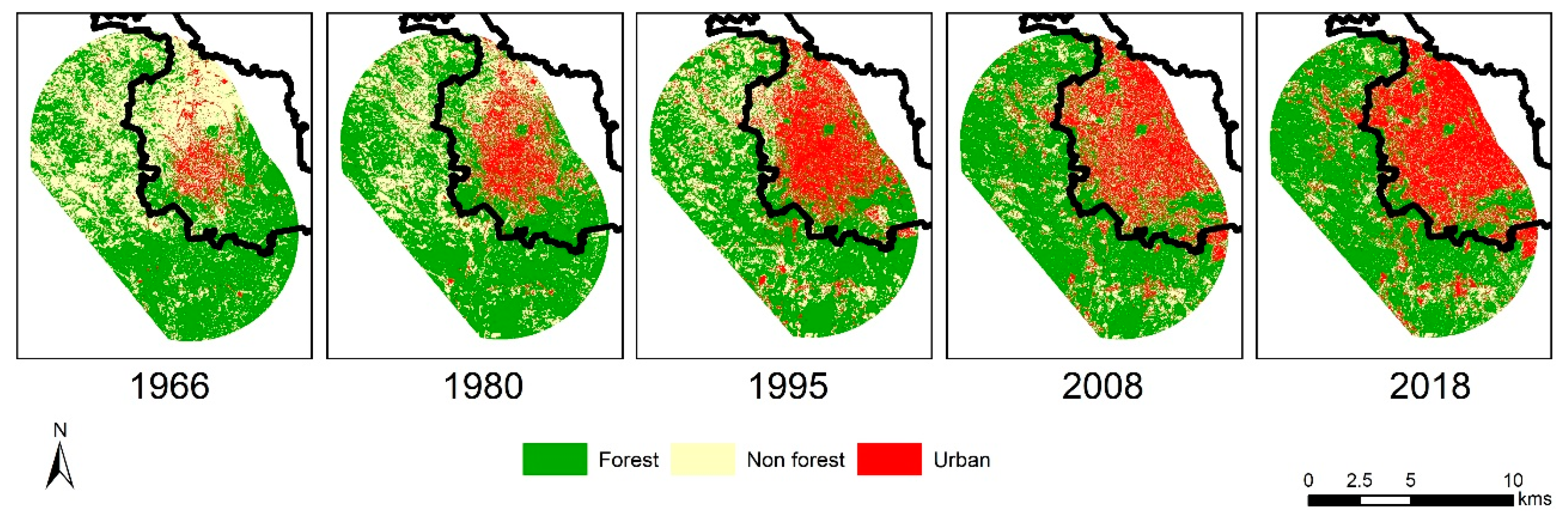
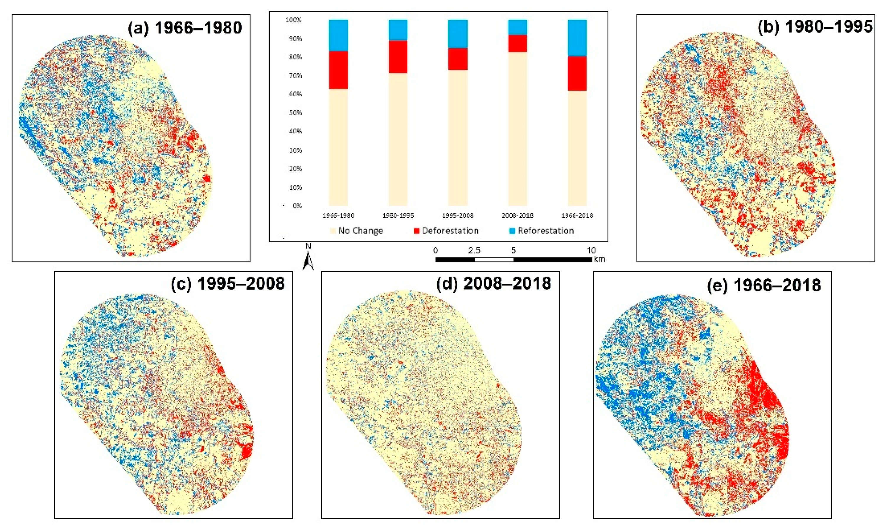
3.1. LULC and Analysis of Forest Cover Change

The satellite image classification of forest cover for all the studied periods had an overall accuracy (i.e., concordance index) of more than 90% between the points verified in the field and the image classification. During the 52-year-period (1966–2018; Figure 2), the net area of forest lost was 1092 ha, with a total annual deforestation rate of −0.004%. Urban area expansion went from 690 ha to 3290 ha. The 1966–1980 period displayed the lowest loss of forest cover (151.23 ha), even though it comprised 14 years. In contrast, the most significant loss of forest cover (513.56 ha; Table 2) occurred between 1980–1995 (15 years).
Between 1966 and 1980, an area of 2132 ha exhibited tree recovery, mainly on former agricultural and cattle-ranching areas. This reforested area decreased to only 958 ha by 2018, with other losses in each period (Figure 3). Forest loss from the pre-existing tree growth in 1966 was unclear and fluctuated among periods, as shown in Figure 2. The lowest rate (11 ha/year) was recorded during the 1966–1980 period. Next, the deforestation rate increased three times to its highest value (34 ha/year), recorded between 1980 and 1995. A decrease of almost 50% (18.2 ha/year) followed in 1995–2008, increasing again between 2008 and 2018, reaching 28 ha/year. New forests and deforested areas had a particular spatial distribution according to the period studied; for instance, forest recovery was present mainly in the western and northwestern sectors of the peri-urban zone of Xalapa city between 1966–1980 and 1995–2008, while the deforestation was more intense toward the east and southeast. In contrast, the spatial distribution of intense deforestation shifted between 1980 and 1995 to the city’s limits and the peri-urban southern sector.
The images highlight that deforestation and forest recovery occurred throughout the study area, without any clear trend during the last analyzed period, i.e., 2008–2018. However, remarkable recuperation (northwest) and deforestation (south and southeast) tendencies were observed when 1966 and 2018 were compared (Figure 1 and Figure 3). Xalapa grew from 610 ha in 1966 to 3279 ha in 2018, mainly over pastures/crops (1489 ha) and forest areas (987 ha). In 2018, the remaining forest occupied 6628 ha, and livestock or agricultural activities were still carried out in 2158 ha.

3.2. Potential Drivers of Forest Change

The logistic regression showed that some social and biophysical variables had a significant relationship with forest recovery or deforestation (Table 3). Elevation (m.a.s.l.), distance from the forest edge, distance to urban limits (labeled urban distance), and population density were significant variables for forest recovery and deforestation. However, the direction of the correlation was the opposite in most cases. For example, while deforestation was more significant the closer one is to the edge of the forest, regeneration was more significant the further one was from the edge. However, there also existed variables that only appeared during deforestation or forest recovery. In deforestation, the kind of land tenure (ejido vs. private) and margination were unique variables to deforestation. In comparison, precipitation and slope were the sole variables exclusive of forest recovery.
The unique variable present in all deforestation and forest recovery periods was the urban distance, negatively associated with forest loss and positively with forest recovery. However, not all periods were significant; in the case of deforestation, only the period of 1966–1980 was significant, and for forest recovery, the periods of 1995–2008 and 2008–2018 were significant. Distance to forest edge was the only significant explanatory variable retained in models for all study periods (Table 3). This variable was negatively associated with forest loss but positively associated with forest recovery. The population density was positively associated with deforestation in almost every period (except 1980–1995). It was negatively associated with forest recovery in 1995–2008 and 2008–2018.

4. Discussion

The main findings of our study suggest the importance of evaluating the long-term loss–recovery forest dynamics in peri-urban landscapes and urban areas and the multiple variables (biophysical and socioeconomic) involved. For example, in the case of Xalapa, 1090 ha of forest were lost (in net terms) in 52 years, which is 8% of the total study area and could be considered lower than expected. Our logistic regression analysis showed that distance to forest edge was a significant explanatory variable for forest recovery and deforestation during all of the studied transition periods. Precipitation and slope were significant biophysical variables, and the land property type was highlighted among the socioeconomic variables. The results also highlight the importance of investing in and producing up-to-date information on the quantity and quality of land-use changes and vegetation cover.
A low net forest loss was related to the study area’s high loss–recovery dynamics. Consequently, the city’s growth took place on agricultural land and forest, but simultaneously, the forest was recovered in some areas, partially offsetting the loss [23]. Causes of deforestation or forest recovery varied in time and region [45]. Forest clearing occurs mainly on edge between forested and open areas, which explains the significant and negative relationship between deforestation and distance to the forest edge in all periods [46,47,48]. Previous studies also found that deforestation increases in areas near the forest’s edge, likely due to greater accessibility and lower transportation costs [47,48]. Thus, promoting conservation strategies that protect areas near the forest edge may be advisable.
In a peri-urban landscape, large open spaces predominate, such as forests, farmland, roads, and other areas with a lower population density but which functionally belong to the urban area [49]. These open spaces have three options for change: continue to be pastures/crops, recover their vegetation cover, or become human settlements. Therefore, these open spaces are fundamental to developing sustainable strategies that promote human well-being in these areas [50]. Under an ecosystem-based management approach, these open spaces are crucial to biodiversity conservation, temperature regulation, noise reduction, and water management, which directly benefit human well-being. For example, our results suggest that from 1966 to 2018 in the northwest, the significant transitions of these open spaces were from grasslands/crops to the expansion of human settlements and vegetation recovery. Nevertheless, in the southwest, the transitions were mainly towards deforestation and the development of human settlements. These changes will affect the structure and functionality of the landscape; wherein the northwest, the effects of urban growth will possibly be cushioned by reforestation, but in the case of the southwest, the impacts of the loss of vegetation and increase in human settlements will have adverse effects for society.
Two important biophysical variables were precipitation and slope. In the first case, the effects were evident in the higher forest recovery rates during 1966–1980 and 1995–2008 when precipitation was higher. This effect could be related to the dominant vegetation, cloud forest, in the peri-urban landscape. In this vegetation type, precipitation-related variables and mean temperature have been identified as critical factors controlling forest-type distribution on mountains and defining altitudinal ecological gradients. It is well-known that woody plants’ growth and establishment success are higher in more humid areas, particularly close to forest edges. In the second case, slope, economic models developed on the subject predict that better soils and land with low or flat inclines allow for more significant clearing, since landowners prefer to deforest the most productive lands. In turn, forest conservation on land with steep grades presents lower opportunity costs because of a more complex agricultural production and more expensive product transportation [19], thus supporting the decision to invest less in conserving low opportunity cost steep slopes.
According to the logistic regression, a critical socioeconomic variable that influenced deforestation was property type, particularly between 1995 and 2008. Similarly, previous studies suggest that the socioeconomic context of communal and private lands can be decisive in land-use decisions, with communal lands producing positive effects on forest conservation [22,51]. In the case of Xalapa, the city grew towards the southeast, where private property predominates. However, more rigorous experimental designs than those used here, such as matching techniques, may also be necessary for detecting these trends [52].
The biophysical and socioeconomic variables identified as triggers of deforestation and forest recovery highlight the importance of including dynamic and socio-ecological dimensions to study complex landscapes. In this sense, the inclusion of landscape ecology, which focuses on understanding how natural and anthropic gradients modify the spatial distribution of socio-ecological systems, must be included in urban planning practices. Understanding urban and peri-urban landscape dynamics enables the design of mechanisms and adaptation measures to enhance planning processes where essential ES must be provided to inhabitants’ well-being in current and climate change scenarios. Therefore, it is necessary to increase studies that link peri-urban landscapes and urban areas to determine conservation strategies and design adaptation measures.
In Mexico, cities that seek to be resilient must face the challenge of contending, strategically and responsibly, with the accelerated change in land use triggering the physical expansion of formal and informal urbanization [29]. In metropolitan areas, the direct pressure exerted by factors associated with economic, demographic, and sociocultural dynamics puts the ecological and functional integrity of green areas such as urban and peri-urban forests at risk.
High-quality green spaces are a hallmark of a sustainable city, as they epitomize good planning and management and a healthy environment for humans, vegetation, and wildlife populations. The city of Xalapa has relatively abundant vegetation. However, this could change due to the accelerated growth of the city; for this reason, it is essential to identify these areas to prioritize them in conservation or restoration programs. Quantifying the role of this undervalued vegetation type in generating benefits for society remains a priority for future research. In this sense, this study contributes evidence of the possibility of recovering forest cover while urban areas are growing. Since the development of a city is usually directly linked to deforestation, strategic management measures, such as reforestation [24] focused on recovering ES crucial to urban inhabitants’ well-being, are needed.
The methodological caveats and limitations to consider in this study include the insufficient availability of high spatial resolution images for the 1960s–1980s and the low spectral resolution in the CORONA images and aerial photographs, which only have the panchromatic band. Both caveats affect the differentiation between categories of vegetation types. Furthermore, vegetation age could be determined if direct field measurements are included and long-term field monitoring efforts are promoted. Long-term field monitoring is needed to evaluate urban and peri-urban forests’ structure, composition, function, and resilience. Furthermore, there is no biophysical and socioeconomic information available for all the study areas (i.e., ground boundary setting, investment, and location of all conservation programs, among others), or the data is frequently outdated.
Despite the limitations mentioned above, this type of analysis remains a valid approximation to understand landscape dynamics in forest recovery and deforestation processes. Likewise, identifying the biophysical and socioeconomic variables meaningful for specific processes is valuable to design and implement better conservation, restoration, and management strategies in peri-urban areas. The long-term resolution, such as the study of 50 years of changes, is crucial to designing measures focused on enhancing ecosystem functioning where urban areas are expanding [53]. This shift in the spatial dynamic of LULC and deforestation or forest recovery drivers creates new opportunities for conserving tropical forests in a context in which conservation organizations can have more information toward adapting their conservation strategies [54].

5. Conclusions

Neotropical landscapes are highly vulnerable to resulting from processes of exploitation, colonization, deforestation, fragmentation, and extraction of non-timber resources [55]. However, these factors change over time, and few studies have evaluated high temporal resolutions (more than 30 years) or included the society–ecosystem interaction through a set of different variables. Our results, obtained from the analysis of more than five decades of landscape dynamics, highlight that the city’s growth modifies the landscape but does not always imply the complete substitution of natural ecosystems. Some cities’ growth, such as Xalapa, indeed promoted forest recovery in the peri-urban landscape. Subsequently, the smart integration of landscape ecology and urban planning is critical to implementing strategies to find and accomplish win–win scenarios, where resilient and adaptative socioecosystems and landscapes could be achieved.
A fundamental aspect of achieving urban resilience is the recovery of degraded ecosystems by urban afforestation actions with native species and protecting still intact forest stands. To this end, cities should invest in information systems whose contents strengthen monitoring and evaluation programs dealing with land-use change and urban growth on natural environments, identify forest areas that can be subject to ecological protection, and promote a privileged standing for green areas within urban planning instruments.
Moreover, decision-makers and researchers alike should remain well aware that this type of analysis, through the use of remote sensing, does have significant limitations [56,57]. These include the lack of required data layers to adequately take into account socioeconomic variables, the choice of scale(s) suitable for analyses, the accuracy of layers used in the model generation, temporal public policies, or market-based decisions that could affect the trends in LULC and, therefore, the performance of this type of influences [16]. For this reason, every effort to complement this type of study with direct field measurements of ES, such as water quality, carbon sequestration, or biodiversity, through monitoring and interviews, should be made.
The spatial analysis metrics presented throughout this study have been valuable in analyzing, monitoring, and following landscape changes, including critical drivers such as urban growth. Furthermore, these methods allowed the study case analysis from different lenses, ranging from the description of these landscapes, to comparing simulations of urban occupations and land-use changes. Studies of this type could deeply contribute to land-use planning through monitoring landscape changes in urban and peri-urban observatories.

Author Contributions

Conceptualization, J.V.T., G.B.-C., O.P.-M. and D.L.; methodology, J.V.T. and D.L.; software, J.V.T., O.P.-M. and D.L.; validation, J.V.T. and G.B.-C.; formal analysis, J.V.T. and D.L.; investigation, J.V.T., G.B.-C., O.P.-M. and D.L.; resources, J.V.T., G.B.-C., O.P.-M. and D.L.; data curation, J.V.T.; writing—original draft preparation, J.V.T. and D.L.; writing—review and editing, J.V.T., G.B.-C., O.P.-M. and D.L.; visualization, J.V.T. and D.L.; supervision, O.P.-M.; project administration, O.P.-M.; funding acquisition, J.V.T., G.B.-C. and O.P.-M. All authors have read and agreed to the published version of the manuscript.

Funding

J.V.T. thanks CONACyT for the grant that supported the development of his postdoctoral fellowship (#483941). This study was supported by remaining funds, project no. 34311656 financed by Universidad Autonoma Metropolitana (UAM), whose head is Gilberto Sven Binnquist Cervantes, and the project i-Gamma (no. 296842) financed by the Mexican National Science and Technology Council (CONACyT)-FORDECyT.

Institutional Review Board Statement

Not applicable.

Informed Consent Statement

Not applicable.

Data Availability Statement

The datasets generated during and/or analyzed during the current study are available from J.V.T. and D.L. on reasonable request.

Acknowledgments

We are grateful to Rosario Landgrave for her kind support with image processing and to Citlalli González Hernández for assisting in editing the manuscript. The authors express their gratitude to Fabiola López-Barrera for their thorough comments and recommendations. We are also grateful to the anonymous reviewers.

Conflicts of Interest

The authors declare no conflict of interest.

References

  1. FAO. El Estado de los Bosques Del Mundo 2020: Los Bosques, La Biodiversidad Y Las Personas; FAO: Roma, Italy, 2020. [Google Scholar]
  2. Daily, G.C. Nature’s services: Societal dependence on natural ecosystems. In Introduction: What Are Ecosystem Services; Yale University Press: New Haven, CT, USA, 1997. [Google Scholar]
  3. IUCN. Policy Brief on the Economics of Forest Landscape Restoration; International Union for Conservation of Nature: Gland, Switzerland, 2020. [Google Scholar]
  4. Brockerhoff, E.G.; Barbaro, L.; Castagneyrol, B.; Forrester, D.I.; Gardiner, B.; González-Olabarria, J.R.; Lyver, P.O.B.; Meurisse, N.; Oxbrough, A.; Taki, H.; et al. Forest Biodiversity, Ecosystem Functioning and the Provision of Ecosystem Services. Biodivers. Conserv. 2017, 26, 3005–3035. [Google Scholar] [CrossRef] [Green Version]
  5. Borrelli, P.; Robinson, D.A.; Fleischer, L.R.; Lugato, E.; Ballabio, C.; Alewell, C.; Meusburger, K.; Modugno, S.; Schütt, B.; Ferro, V.; et al. An assessment of the global impact of 21st century land use change on soil erosion. Nat. Commun. 2017, 8, 2013. [Google Scholar] [CrossRef] [PubMed] [Green Version]
  6. Dlamini, C.S. Contribution of Forest Ecosystem Services toward Food Security and Nutrition; Walter, L.F., Anabela, M.A., Luciana, B.P., Gökçin, Ö., Tony, W., Eds.; Springer International Publishing: Cham, Switzerland, 2020; pp. 179–196. [Google Scholar]
  7. FAO. State of the World’s Forests 2016. Forests and Agriculture: Land-Use Challenges and Opportunities; FAO: Roma, Italy, 2016. [Google Scholar]
  8. Dudley, N.; Sue, S. Running Pure: The Importance of Forest Protected Areas to Drinking Water; World Bank/WWF Alliance for Forest Conservation and Sustainable Use: Washington, DC, USA, 2003. [Google Scholar]
  9. Austin, K.G.; Baker, J.S.; Sohngen, B.L.; Wade, C.M.; Daigneault, A.; Ohrel, S.B.; Ragnauth, S.; Bean, A. The economic costs of planting, preserving, and managing the world’s forests to mitigate climate change. Nat. Commun. 2020, 11, 5946. [Google Scholar] [CrossRef] [PubMed]
  10. IPBES. Summary for Policymakers of the Global Assessment Report on Biodiversity and Ecosystem Services of the Intergovernmental Science-Policy Platform on Biodiversity and Ecosystem Services; IPBES: Bonn, Germany, 2019. [Google Scholar]
  11. De Fries, R.; Achard, F.; Brown, S.; Herold, M.; Murdiyarso, D.; Schlamadinger, B.; de Souza, C. Earth observations for estimating greenhouse gas emissions from deforestation in developing countries. Environ. Sci. Policy 2007, 10, 385–394. [Google Scholar] [CrossRef]
  12. UN. Decade on Restoration. Available online: https://www.decadeonrestoration.org/strategy (accessed on 27 February 2022).
  13. Foley, J.A.; DeFries, R.; Asner, G.P.; Barford, C.; Bonan, G.; Carpenter, S.R.; Chapin, F.S.; Coe, M.T.; Daily, G.C.; Gibbs, H.K.; et al. Global consequences of land use. Science 2005, 309, 570–574. [Google Scholar] [CrossRef] [PubMed] [Green Version]
  14. Geist, H.J.; Lambin, E.F. Proximate Causes and Underlying Driving Forces of Tropical Deforestation: Tropical Forests Are Disappearing as the Result of Many Pressures, Both Local and Regional, Acting in Various Combinations in Different Geographical Locations. BioScience 2002, 52, 143–150. [Google Scholar] [CrossRef]
  15. Von Thaden, J.J.; Laborde, J.; Guevara, S.; Venegas-Barrera, C.S. Forest cover change in the Los Tuxtlas Biosphere Reserve and its future: The contribution of the 1998 protected natural area decree. Land Use Policy 2018, 72, 443–450. [Google Scholar] [CrossRef]
  16. De Groot, R.S.; Alkemade, R.; Braat, L.; Hein, L.; Willemen, L. Challenges in integrating the concept of ecosystem services and values in landscape planning, management and decision making. Ecol. Complex. 2010, 7, 260–272. [Google Scholar] [CrossRef]
  17. Seto, K.C.; Güneralp, B.; Hutyra, L.R. Global Forecasts of Urban Expansion to 2030 and Direct Impacts on Biodiversity and Carbon Pools. Proc. Natl. Acad. Sci. USA 2012, 109, 16083–16088. [Google Scholar] [CrossRef] [Green Version]
  18. Rosero-Bixby, L.; Palloni, A.; Poblacion, Y. Deforestacion En Costa Rica, Conservacion Del Bosque En Costa Rica; Academia Nacional de Ciencias: San Jose, CA, USA, 1998. [Google Scholar]
  19. Leguía Aliaga, J.D.; Villegas Quino, H.; Aliaga Lordemann, J. Deforestación En Bolivia: Una Apro-ximación Espacial. Rev. Latinoam. Desarro. Económico 2011, 15, 7–44. [Google Scholar]
  20. Osorio, L.P.; Mas, J.F.; Guerra, F.; Maass, M. Análisis Y Modelación de Los Procesos de Deforestación: Un Caso de Estudio En La Cuenca Del Río Coyuquilla, Guerrero, México. Investig. Geográficas 2015, 88, 60–74. [Google Scholar]
  21. Yackulic, C.B.; Fagan, M.; Jain, M.; Jina, A.; Lim, Y.; Marlier, M.; Muscarella, R.; Adame, P.; DeFries, R.; Uriarte, M. Biophysical and Socioeconomic Factors Associated with Forest Transitions at Multiple Spatial and Temporal Scales. Ecol. Soc. 2011, 16, 15. [Google Scholar] [CrossRef] [Green Version]
  22. Bonilla-Moheno, M.; Aide, T.M.; Clark, M.L. The influence of socioeconomic, environmental, and demographic factors on municipality-scale land-cover change in Mexico. Reg. Environ. Chang. 2011, 12, 543–557. [Google Scholar] [CrossRef]
  23. Aide, T.M.; Clark, M.L.; Grau, H.R.; López-Carr, D.; Levy, M.A.; Redo, D.; Bonilla-Moheno, M.; Riner, G.; Andrade-Núñez, M.J.; Muñiz, M. Deforestation and Reforestation of Latin America and the Caribbean (2001–2010). Biotropica 2013, 45, 262–271. [Google Scholar] [CrossRef]
  24. Abadie, J.; Dupouey, J.-L.; Avon, C.; Rochel, X.; Tatoni, T.; Bergès, L. Forest recovery since 1860 in a Mediterranean region: Drivers and implications for land use and land cover spatial distribution. Landsc. Ecol. 2017, 33, 289–305. [Google Scholar] [CrossRef]
  25. Honey-Rosés, J.; Maurer, M.; Ramírez, M.I.; Corbera, E. Quantifying active and passive restoration in Central Mexico from 1986–2012: Assessing the evidence of a forest transition. Restor. Ecol. 2018, 26, 1180–1189. [Google Scholar] [CrossRef]
  26. Ellis, E.A.; Romero Montero, A.; Hernández Gómez, I.U. Evaluación Y Mapeo de los Determinantes de Deforestación En La Pe-nínsula Yucatán; Agencia de los Estados Unidos para el Desarrollo Internacional, The Nature Conservancy, Alianza México REDD+, México; Distrito Federal: Mexico City, México, 2015. [Google Scholar]
  27. García-Ayllón, S. Rapid development as a factor of imbalance in urban growth of cities in Latin America: A perspective based on territorial indicators. Habitat Int. 2016, 58, 127–142. [Google Scholar] [CrossRef]
  28. Schumacher, M.; Durán-Díaz, P.; Kurjenoja, A.K.; Gutiérrez-Juárez, E.; González-Rivas, D.A. Evolution and Collapse of Ejidos in Mexico—To What Extent Is Communal Land Used for Urban Development? Land 2019, 8, 146. [Google Scholar] [CrossRef] [Green Version]
  29. Tellman, B.; Eakin, H.; Janssen, M.A.; de Alba, F.; Ii, B.T. The role of institutional entrepreneurs and informal land transactions in Mexico City’s urban expansion. World Dev. 2021, 140, 105374. [Google Scholar] [CrossRef]
  30. Bertzky, B.; Shi, Y.; Hughes, A.; Engels, B.; Ali, M.K.; Badman, T. Terrestrial Biodiversity and the World Heritage List: Identifying Broad Gaps and Potential Candidate Sites for Inclusion in the Natural World Heritage Network; Unep-Wcmc: Cambridge, UK, 2013. [Google Scholar]
  31. Gámez, N.; Escalante, T.; Rodríguez, G.; Linaje, M.; Morrone, J.J. Caracterización Biogeográfica de la Faja Volcánica Transmexicana Y Análisis de Los Patrones de Distribución de Su Mastofauna. Rev. Mex. Biodivers. 2012, 83, 258–272. [Google Scholar] [CrossRef] [Green Version]
  32. Morrone, J.J. Fundamental biogeographic patterns across the Mexican Transition Zone: An evolutionary approach. Ecography 2010, 33, 355–361. [Google Scholar] [CrossRef]
  33. Arriaga-Jiménez, A.; Rös, M.; Halffter, G. High variability of dung beetle diversity patterns at four mountains of the Trans-Mexican Volcanic Belt. PeerJ 2018, 6, e4468. [Google Scholar] [CrossRef] [PubMed] [Green Version]
  34. SEMARNAT. Informe De La Situación Del Medio Ambiente En México; Compendio De Estadísticas Ambientales; SE-MARNAT and PNUD: Mexico City, Mexico, 2005. [Google Scholar]
  35. SEDATU. Reglas De Operación Del Programa De Mejoramiento Urbano, Para El Ejercicio Fiscal 2019; Diario Oficial de la Federación: Mexico City, Mexico, 2019. [Google Scholar]
  36. Benítez, G.; Pérez-Vázquez, A.; Nava-Tablada, M.; Equihua, M.; Álvarez-Palacios, J.L. Urban Expansion and the Environmental Effects of Informal Settlements on the Outskirts of Xalapa City, Veracruz, Mexico. Environ. Urban 2012, 24, 149–166. [Google Scholar] [CrossRef]
  37. Balderas Torres, A.; Angón Rodríguez, S.; Sudmant, A.; Gouldson, A. Adapting to Climate Change in Mountain Cities: Lessons from Xalapa, Mexico; Coalition for Urban Transitions: Xalapa, Mexico, 2021. [Google Scholar]
  38. Lemoine-Rodríguez, R.; MacGregor-Fors, I.; Muñoz-Robles, C. Six decades of urban green change in a neotropical city: A case study of Xalapa, Veracruz, Mexico. Urban Ecosyst. 2019, 22, 609–618. [Google Scholar] [CrossRef]
  39. INEGI. Continuo De Elevaciones Mexicano (Cem); INEGI: Mexico City, Mexico, 2013. [Google Scholar]
  40. Campbell, M.; Congalton, R.G.; Hartter, J.; Ducey, M. Optimal Land Cover Mapping and Change Analysis in Northeastern Oregon Using Landsat Imagery. Photogramm. Eng. Remote Sens. 2015, 81, 37–47. [Google Scholar] [CrossRef] [Green Version]
  41. Congalton, R.G.; Green, K. Assessing the Accuracy of Remotely Sensed Data: Principles and Practices; CRC Press: Boca Raton, FL, USA, 2019. [Google Scholar]
  42. Puyravaud, J.-P. Standardizing the calculation of the annual rate of deforestation. For. Ecol. Manag. 2003, 177, 593–596. [Google Scholar] [CrossRef]
  43. Ludeke, A.K.; Maggio, R.C.; Reid, L.M. An analysis of anthropogenic deforestation using logistic regression and GIS. J. Environ. Manag. 1990, 31, 247–259. [Google Scholar] [CrossRef]
  44. Echeverria, C.; Coomes, D.A.; Hall, M.; Newton, A.C. Spatially explicit models to analyze forest loss and frag-mentation between 1976 and 2020 in southern Chile. Ecol. Model. 2008, 212, 439–449. [Google Scholar] [CrossRef]
  45. Gibbs, H.K.; Johnston, M.; A Foley, J.; Holloway, T.; Monfreda, C.; Ramankutty, N.; Zaks, D. Carbon payback times for crop-based biofuel expansion in the tropics: The effects of changing yield and technology. Environ. Res. Lett. 2008, 3, 034001. [Google Scholar] [CrossRef]
  46. Skole, D.; Tucker, C. Tropical Deforestation and Habitat Fragmentation in the Amazon: Satellite Data from 1978 to 1988. Sci. 1993, 260, 1905–1910. [Google Scholar] [CrossRef] [Green Version]
  47. Ranta, P.; Blom, T.O.M.; Joensuu, E.; Siitonen, M. The Fragmented Atlantic Rain Forest of Brazil: Size, Shape and Distribution of Forest Fragments. Biodivers. Conserv. 1998, 7, 385–403. [Google Scholar] [CrossRef]
  48. Cochrane, M.A. Synergistic Interactions between Habitat Fragmentation and Fire in Evergreen Tropical Forests. Conserv. Biol. 2001, 15, 1515–1521. [Google Scholar] [CrossRef]
  49. Wandl, A.; Magoni, M. Sustainable Planning of Peri-Urban Areas: Introduction to the Special Issue. Plan. Pract. Res. 2017, 32, 1–3. [Google Scholar] [CrossRef] [Green Version]
  50. Reyes-Riveros, R.; Altamirano, A.; de La Barrera, F.; Rozas-Vásquez, D.; Vieli, L.; Meli, P. Linking public urban green spaces and human well-being: A systematic review. Urban For. Urban Green. 2021, 61, 127105. [Google Scholar] [CrossRef]
  51. Salas-Morales, S.H.; Meave, J.A. Elevational patterns in the vascular flora of a highly diverse region in southern Mexico. Plant Ecol. 2012, 213, 1209–1220. [Google Scholar] [CrossRef]
  52. Williams-Linera, G.; Toledo-Garibaldi, M.; Hernández, C.G. How heterogeneous are the cloud forest communities in the mountains of central Veracruz, Mexico? Plant Ecol. 2013, 214, 685–701. [Google Scholar] [CrossRef]
  53. Nor, A.N.M.; Corstanje, R.; Harris, J.; Grafius, D.; Siriwardena, G.M. Ecological connectivity networks in rapidly expanding cities. Heliyon 2017, 3, e00325. [Google Scholar] [CrossRef] [Green Version]
  54. Rudel, T.K.; Defries, R.; Asner, G.P.; Laurance, W.F. Changing Drivers of Deforestation and New Opportunities for Conservation. Conserv. Biol. 2009, 23, 1396–1405. [Google Scholar] [CrossRef]
  55. Rodriguez, A.; Gasc, A.; Pavoine, S.; Grandcolas, P.; Gaucher, P.; Sueur, J. Temporal and Spatial Variability of Animal Sound within a Neotropical Forest. Ecol. Inform. 2014, 21, 133–143. [Google Scholar] [CrossRef]
  56. Aukland, L.; Costa, P.M.; Brown, S. A conceptual framework and its application for addressing leakage: The case of avoided deforestation. Clim. Policy 2003, 3, 123–136. [Google Scholar] [CrossRef]
  57. Le Velly, G.; Dutilly, C. Evaluating Payments for Environmental Services: Methodological Challenges. PLoS ONE 2016, 11, e0149374. [Google Scholar] [CrossRef] [PubMed] [Green Version]
Figure 1. Location and boundaries of the study area: the periphery of Xalapa city. Satellite image of 1966 and 2018.
Land 11 00522 g001
Figure 2. Land use and land cover maps from 1966 to 2018 in peri-urban and urban Xalapa city.
Land 11 00522 g002
Figure 3. Transition changes in forest cover for the periods of 1966–1980 (a), 1980–1995 (b), 1995–2008 (c), 2008–2018 (d), and 1966–2018 (e) in the study area.
Land 11 00522 g003
Table 1. Biophysical and socioeconomic explanatory variables used in stepwise logistic regression models explaining patterns of forest cover loss and gain in the peri-urban zone of the city of Xalapa.
VariablesSourceInterpolation Method
Socioeconomic (1) Land tenure (ejido-private)National Agrarian Registry Inverse distance weighting (IDW)
(2) Population density (hab/km²)National Institute of Statistics, Geography and Informatics; (INEGI), census of 1970, 1980, 1990, and 2000 Inverse distance weighting (IDW)
(3) Index of marginalizationCONABIO 1995, 2000, 2005, and 2010. Locality degrees of marginalizationInverse distance weighting (IDW)
(4) Distances from the urban edgeLand Use Maps 1966, 1980, 1995, 2008, and 2018Euclidian distance
(5) Population growthINEGI, census of 1970–1980, 1990–2000, 2000–2010, and 2010–2020Inverse distance weighting (IDW)
(6) Distance to roads (m; paved and unpaved)INEGI 2000, Topographic map (1:50,000)Euclidian distance
Biophysical(7) Elevation (m.a.s.l.) INEGI (2012). DEM of 15 m of resolution*
(8) Slope (degrees)Derived from DEM of INEGI*
(9) Aspect (degrees)Derived of DEM of INEGI*
(10) Distance from forest edge (m)Land Use map, 1966, 1980, 1995, 2008, and 2018Euclidian distance
(11) Average annual rainfall (mm)Weather station. CONAGUAInverse distance weighting (IDW)
(12) Distance to permanent rivers (m)INEGIEuclidian distance
* p < 0.05.
Table 2. Annual deforestation rates (%) and area covered by forest (ha) from 1966 to 2011. The area of forest cover for the initial (A1) and final (A2) years during each transition period are as follows.
PeriodInitial Forest Cover (A1)Final Forest Cover (A2)Cover Change (ha)Years% LostAnnual Rate of Deforestation (r)
1966–19807307.05 7155.82−151.23142.07−0.001
1980–19957235.826722.26−513.56157.10−0.005
1995–20086722.266485.51−236.75133.52−0.003
2008–20186485.516215.13−270.38104.17−0.004
Table 3. Variables best-explaining the patterns of forest loss and forest recovery in stepwise logistic regression models run for the study area during different evaluation periods. Variables are presented in order of importance (according to significance level), together with the type and strength of correlation; also reported are the overall significance levels of the final stepwise logistic regression models and their explanatory power (AUC).
Forest LossForest Recovery
PeriodDriversParameter EstimateMean ModelStd. Deviationp Value ModelAUCPeriodDriversParameter EstimateMean ModelStd. Deviationp Value ModelAUC
1966–1980(Intercept)−0.2591 0.001510.811966–1980Intercept(0.2432) 0.000040.83
Elevation ***−0.00571413143Distance from forest edge (m) ***0.09216817
Population density ***0.002448168Urban distance **0.02779715
Distance from forest edge (m) ***−0.00214011Precipitation **0.022813820.4
Urban distance ***−0.00726717
1980–1995(Intercept)0.3168 0.000070.861980–1995Intercept(0.4034) 0.000020.85
Distance from forest edge (m) ***−0.04533313Distance from forest edge (m) ***0.08986212
Urban distance **0.05115214Urban distance **0.06109318
Marginalization *0.3048−0.90.1Slope *0.034762
1995–2008(Intercept)−0.4256 0.000040.841995–2008Intercept(−0.4085) 0.000030.83
Distance from forest edge (m) ***−0.03113014Precipitation ***0.02691605124
Population density **0.001512910.3Urban distance ***0.02639112
Urban distance **−0.0353116Distance from forest edge (m) ***0.0018608
Private/Ejido land *0.400510.2Elevation **−0.00251605120
Elevation *−0.0019140752Population density **−0.0006725134
2008–2018(Intercept)−0.5847 0.000020.872008–2018Intercept(−0.3483) 0.000020.85
Population density ***0.021518750.5Urban distance ***0.24756317
Distance from forest edge (m) ***−0.01462610Distance from forest edge (m) ***−0.0215454
Marginalization **0.0003−0.40.1Population density **0.00361435101
Urban distance *−0.368093
* p < 0.05; ** p < 0.01; *** p < 0.0001.
Publisher’s Note: MDPI stays neutral with regard to jurisdictional claims in published maps and institutional affiliations.

