
Landscape Conservation Assessment in the Latin American Tropics: Application and Insights from Costa Rica


Abstract
:1. Introduction
2. Materials and Methods
2.1. Assessment Premises and Philosophy
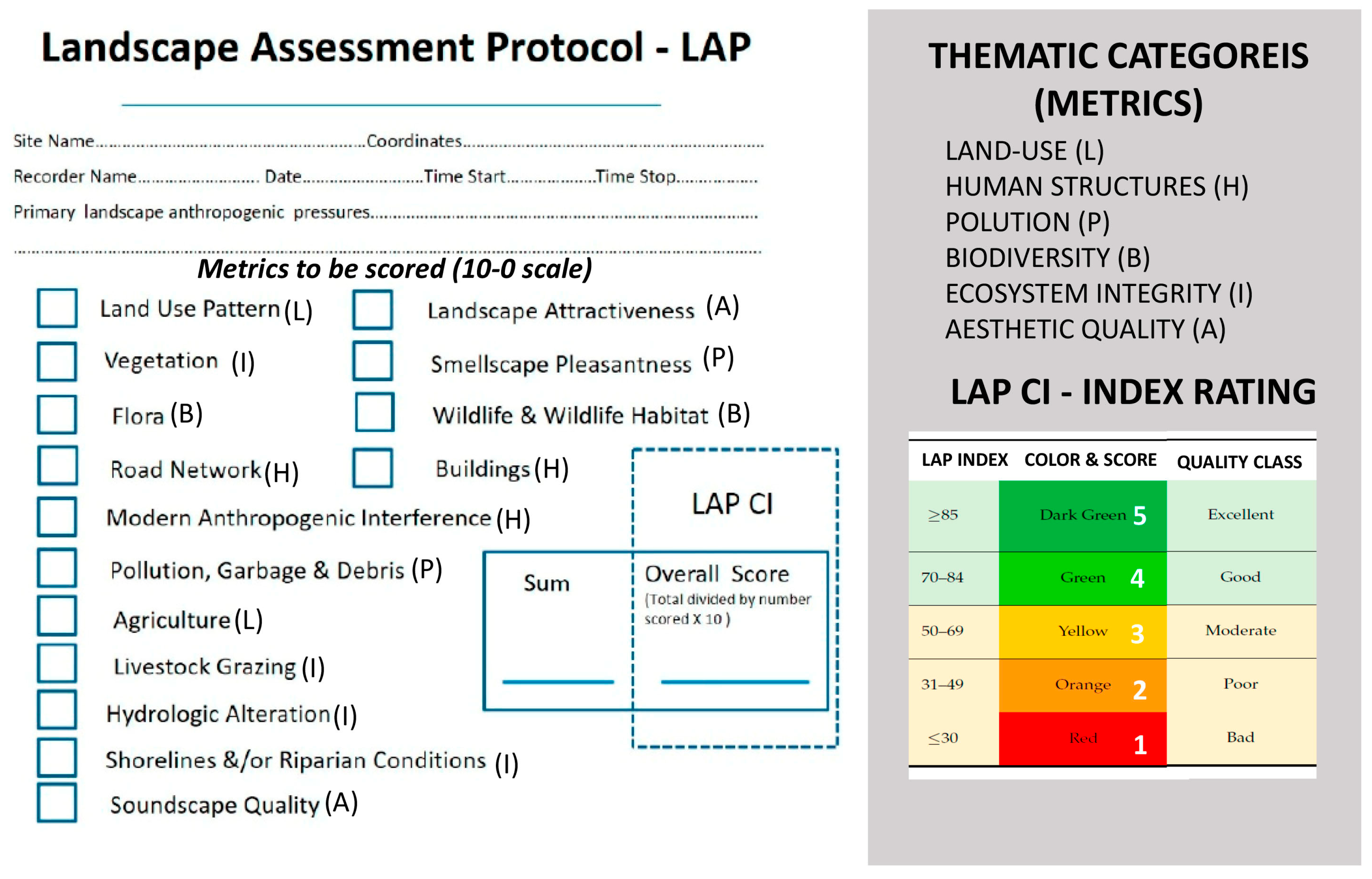
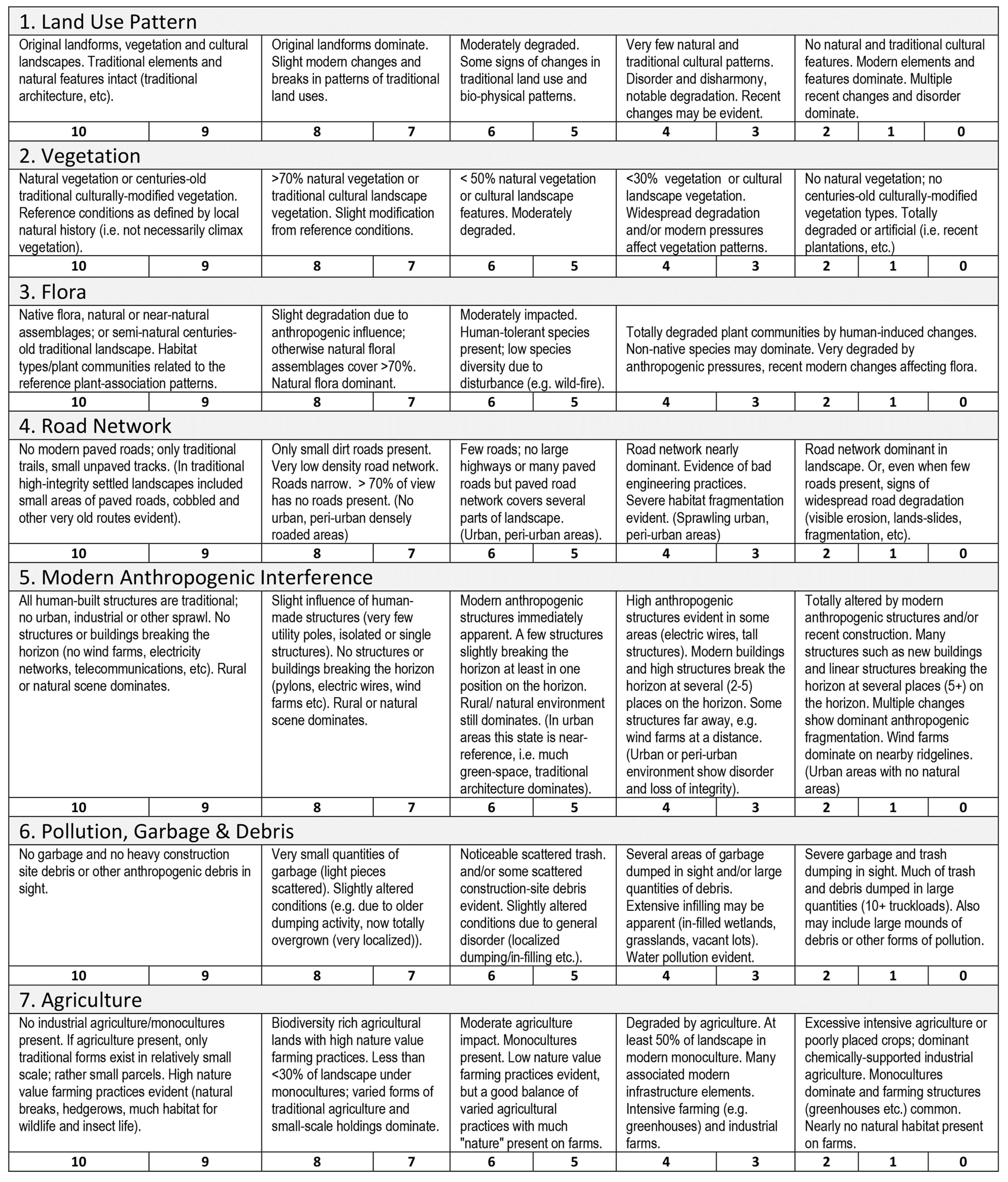
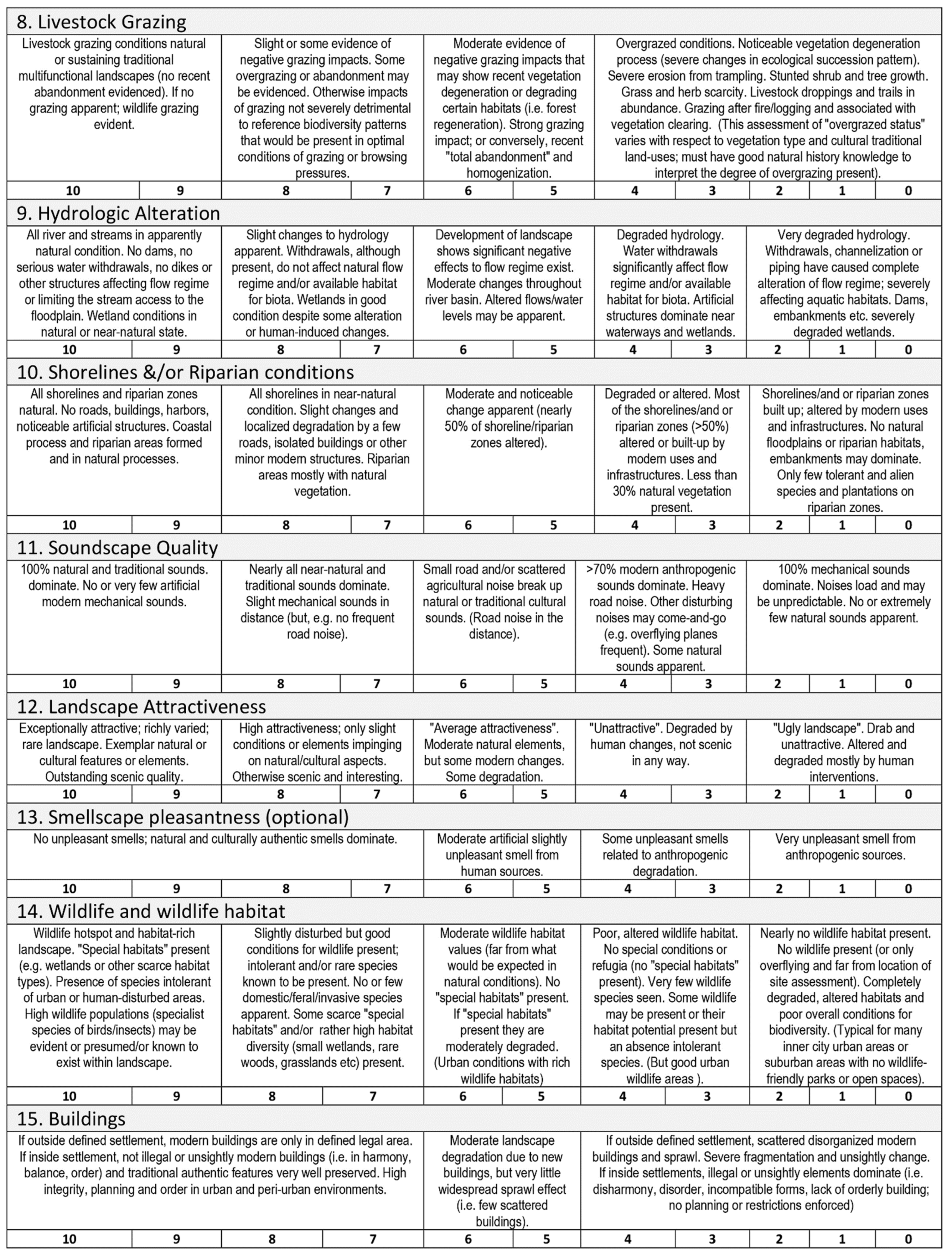
- The approach evaluates landscape view conservation status by examining 15 evaluative criteria (or metrics) for landscape quality. The protocol utilizes different evaluation criteria (metrics) that respond to modern anthropogenic degradation. Each metric refers to different landscape-scale attributes, each having a reference condition state (the “excellent” state, or 10) and a gradient to total degradation conditions (down to “bad”, or 0). The assessor rates the quality of landscape views, not landscape areas (i.e., previously cartographically delineated parcels of land). Only what is perceivable from a viewpoint is assessed.
- Each metric is a quality or characteristic element of the landscape that is known to predictably alter when influenced by human-induced pressures or changes, thus reflecting the quality of a different aspect of the “landscape system”. The metrics cover six different thematic categories: land use, human structures, pollution, biodiversity, ecosystem integrity, and aesthetic quality.
- Each metric is scored by the assessor (or assessors) onsite using a field card (Figure 1) and scoring criteria guidance sheet (Appendix A, Figure A1). A landscape view site must have at least a 180-degree view of the surrounding landscape (assessors can wander up to a 50 m radius from the viewpoint during the assessment). The assessor scores each metric based on the scoring criteria guidance sheet narrative. This code guides the evaluation through an easy-to-use descending score level (i.e., 10 to 0). If an assessor is uncertain how to assess a metric, it should be left without a score. Finally, the LAP provides an integrated semi-quantitative index summarizing the conservation status of the assessed landscape; the LAP index is expressed as a 5-to-1 (excellent to bad) characterization of the landscape view. A trained assessor completes the LAP in about 10 min.
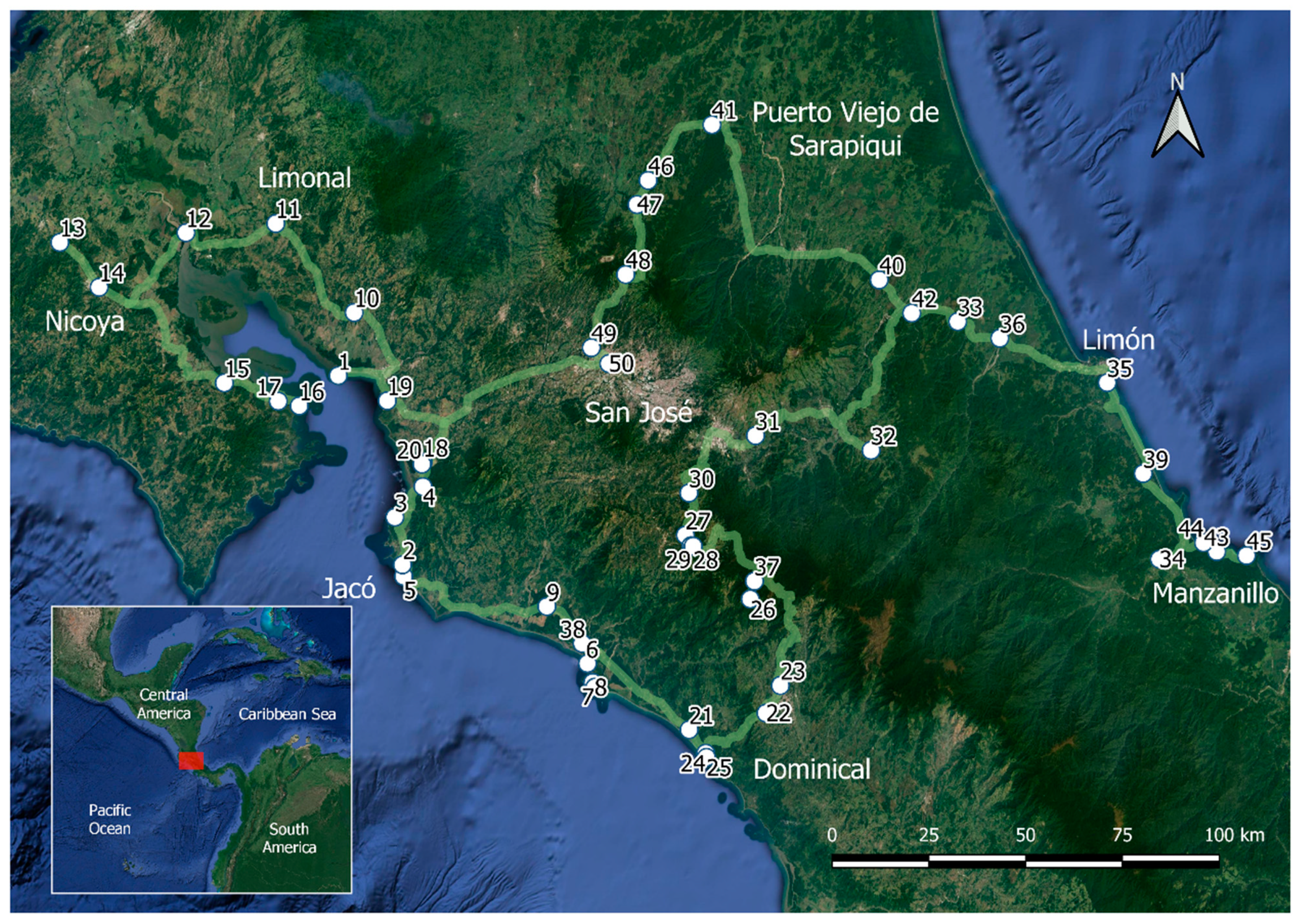
2.2. Study Area
2.3. Application in Costa Rica: Specific On-Site Methods
2.4. Statistical Analyses and Validating Assessments
3. Results
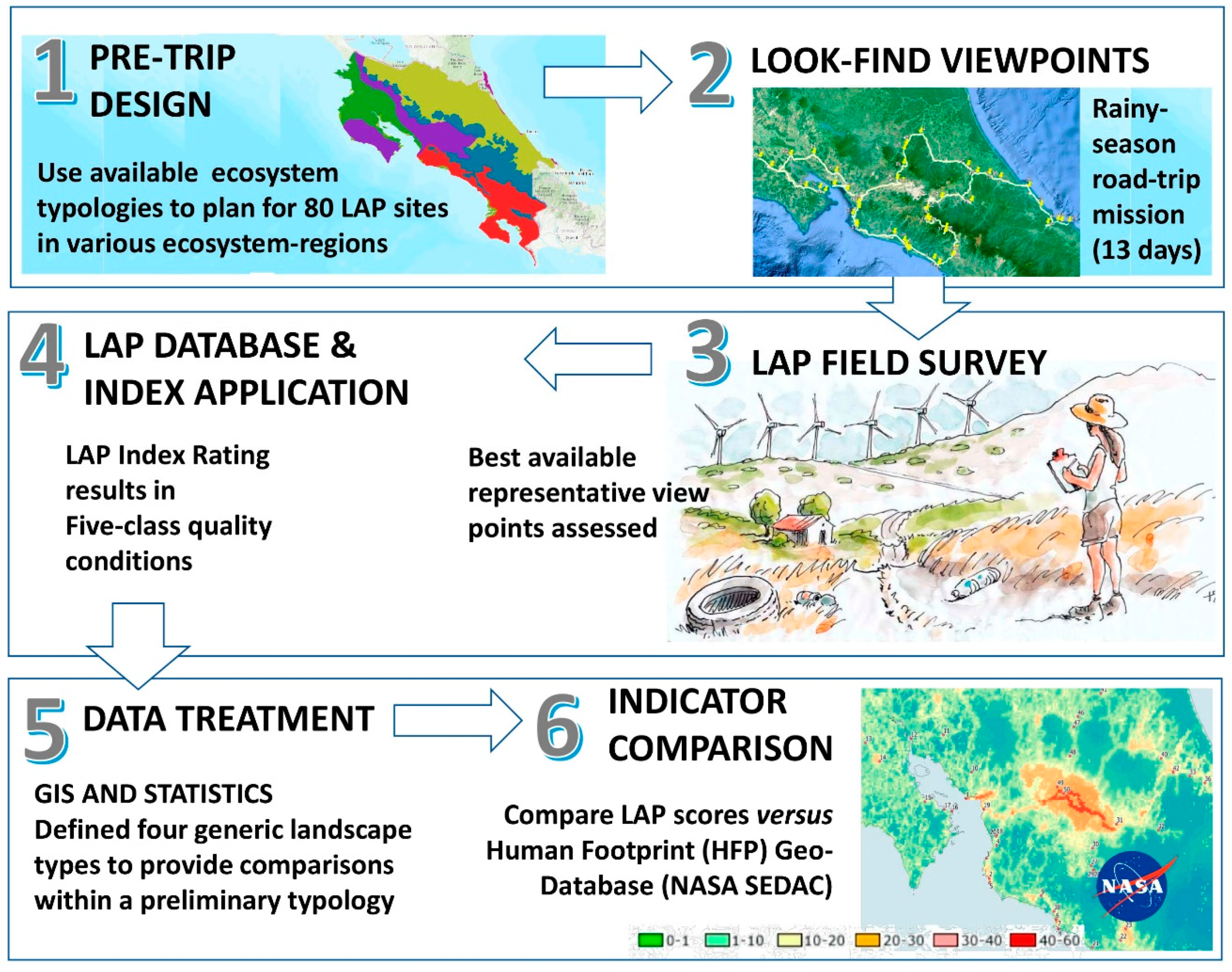
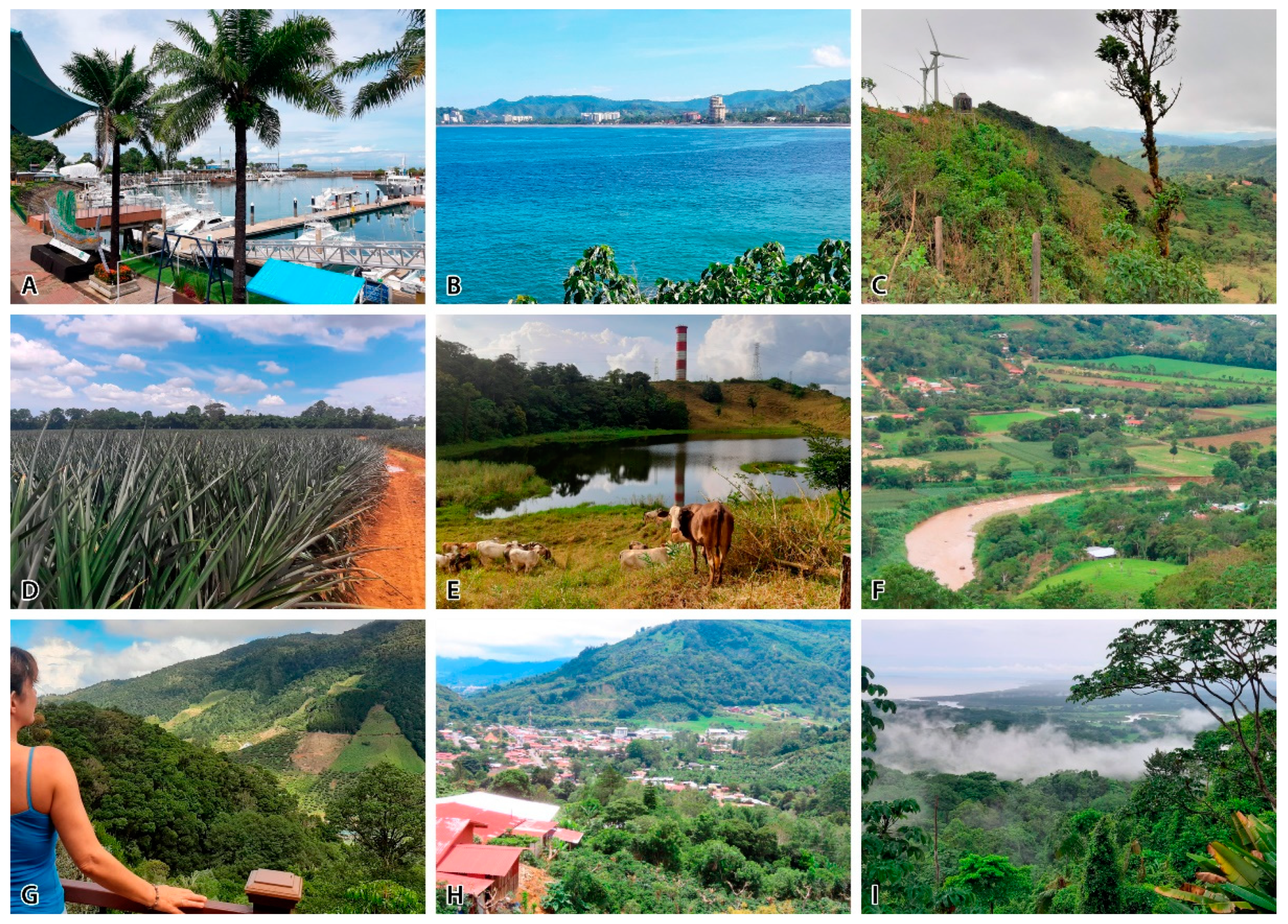
- Coastal (C): immediate contact with and dominance by the coastline;
- Mountain (M): high-relief landscapes, dominated by montane conditions;
- Flatland (F): low-relief landscapes, rolling hills, plains or plateaus;
- Urban/peri-urban (U): dominated by buildings in the immediate vicinity, within or next to settlements.
4. Discussion
4.1. Interpreting Anthropogenic Pressures on Landscapes
4.2. Landscape Metrics Rating Insights and Challenges
4.3. Identifying “Traditional Cultural Landscapes”
4.4. Recommendations
- The use of the LAP as an onsite protocol for landscape view assessments has positive prospects in the tropics of Latin America and could be widely applied as a first-tier screening survey method. The original LAP scoring system provides a standard method and could be used widely without any changes or adaptations. Efforts to better adapt the LAP to regional conditions in the tropics may be investigated after in-depth inquiry. Tweaking the metrics, the numerical class-boundaries, and other aspects of the protocol is a natural evolution of a useful assessment protocol. However, this endeavor should only be started after much evidence is gathered and within a regional intercalibration or standardization process.
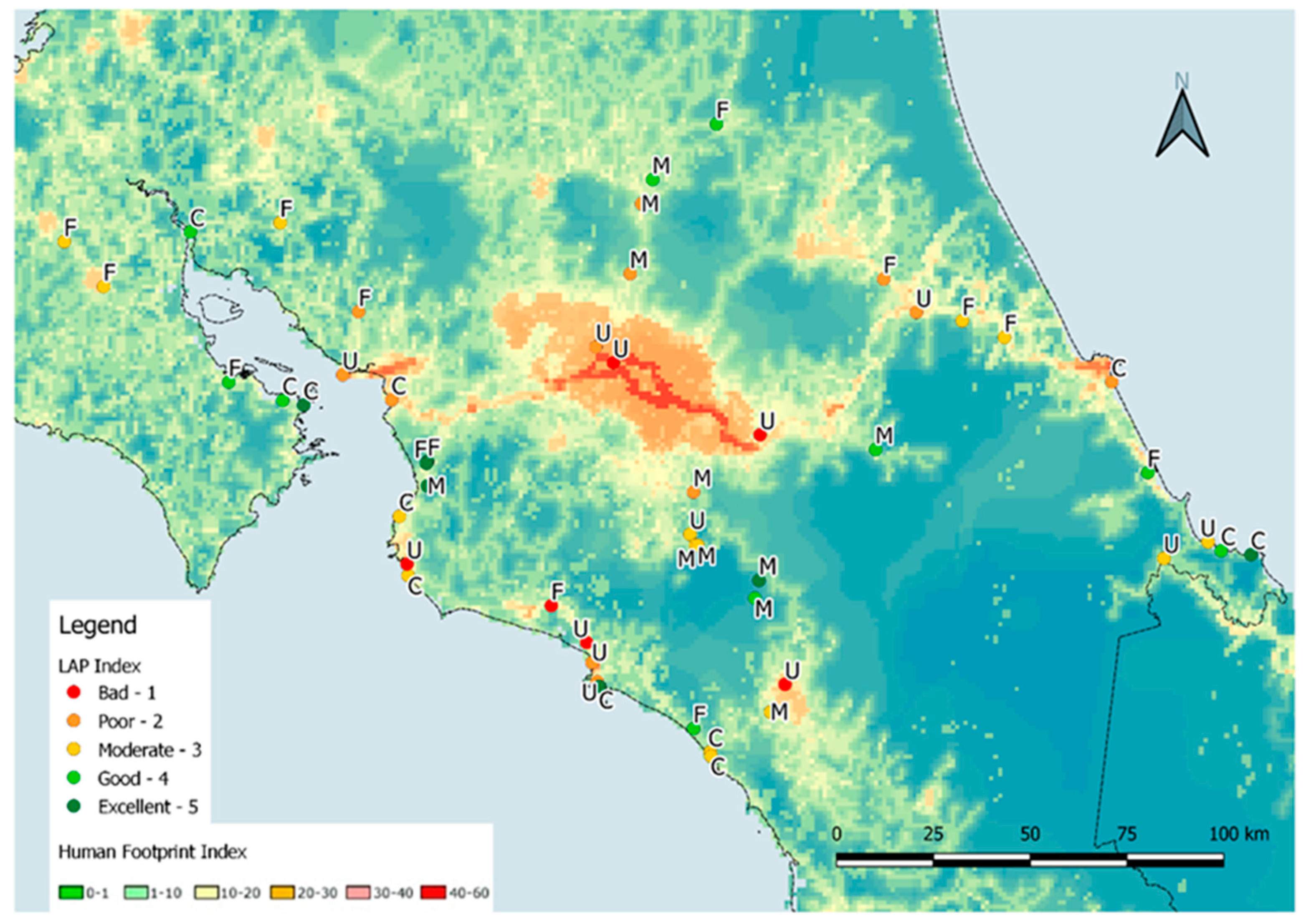
- LAP may combine well with other landscape assessment endeavors (e.g., HFP data); it can be used in “ground truthing” comparisons and in parallel with other approaches that assist in inventory and scoping evaluations of landscapes.
- The inquiry into landscape view assessments may help promote policy recommendations for the preservation and restoration of landscape quality, including a plea for the active promotion of landscape protection measures and restorations outside of protected areas. Economic incentives for landscape restoration may be further incorporated [100].
- Costa Rica and other Latin American countries should seek to pioneer actions to define protected area categories that include the landscapes outside of traditional park designations. A focus on traditional cultural landscapes should be promoted. LAP may help in inventory, assessment, and cartography, as well as in relevant public participation studies.
- Community and citizen participation is important; a key effort must be made to promote landscape literacy and public, student/youth, and resident minority participation. Landscape literacy develops from experience and the LAP provides an onsite tool. A participatory platform such as the LAP could be instrumental for engaging youth, students, locals, and visitors.
5. Conclusions
Author Contributions
Funding
Institutional Review Board Statement
Informed Consent Statement
Data Availability Statement
Acknowledgments
Conflicts of Interest
Appendix A


| SITE # | Longitude (WGS84) | Latitude (WGS84) | Landscape Type | Elevation m.a.s.l. | Date | Site Name |
|---|---|---|---|---|---|---|
| 1 | −84,838632 | 9,973941 | Urban/Peri-Urban | 3 | 6.08.21 | Puntarenas |
| 2 | −84,630709 | 9,614198 | Urban/Peri-Urban | 11 | 8.08.21 | Vista Mar Jaco (near Hotel Del Mar) |
| 3 | −84,665684 | 9,705110 | Coastal | 1 | 8.08.21 | Playa Mantas |
| 4 | −84,605806 | 9,762929 | Mountain | 218 | 8.08.21 | TIKO Mirador Carara |
| 5 | −84,624773 | 9,592389 | Coastal | 14 | 9.08.21 | Mirador Jaco |
| 6 | −84,166989 | 9,426671 | Urban/Peri-Urban | 5 | 9.08.21 | Marina Quepos |
| 7 | −84,149293 | 9,390509 | Urban/Peri-Urban | 10 | 9.08.21 | Manual Antonio Tourist Beach |
| 8 | −84,143438 | 9,381608 | Coastal | 1 | 9.08.21 | Manual Antonio NP Beach |
| 9 | −84,279056 | 9,535017 | Flatland | 21 | 9.08.21 | Rio Palo Seco |
| 10 | −84,820662 | 10,094085 | Flatland | 96 | 10.08.21 | Rancho Grande Gasolinero |
| 11 | −85,033066 | 10,263433 | Flatland | 93 | 10.08.21 | Limonal |
| 12 | −85,248779 | 10,245504 | Coastal | 18 | 10.08.21 | Near Bridge Guanocaste |
| 13 | −85,535678 | 10,227485 | Flatland | 196 | 10.08.21 | Santa Cruz Vikings |
| 14 | −85,429053 | 10,142110 | Flatland | 112 | 10.08.21 | Nikoyia East road |
| 15 | −85,104708 | 9,960166 | Flatland | 17 | 10.08.21 | After Jikarel |
| 16 | −84,921191 | 9,916594 | Coastal | 5 | 10.08.21 | Playa Blanca Nicoyia |
| 17 | −84,970836 | 9,942300 | Coastal | 8 | 10.08.21 | Playa Naranja Nicoyia |
| 18 | −84,612642 | 9,809249 | Flatland | 67 | 10.08.21 | Cerro Lodge Mirador |
| 19 | −84,715533 | 9,926257 | Coastal | 9 | 10.08.21 | Caldera |
| 20 | −84,614791 | 9,805693 | Flatland | 38 | 11.08.21 | Tarcoles river |
| 21 | −83,909294 | 9,301394 | Flatland | 10 | 11.08.21 | Savegre (near Delta) |
| 22 | −83,733139 | 9,332920 | Mountain | 777 | 11.08.21 | Valle Encantado Restaurant |
| 23 | −83,707093 | 9,385252 | Urban/Peri-Urban | 750 | 11.08.21 | San Isidoro El General |
| 24 | −83,863655 | 9,256796 | Coastal | 10 | 11.08.21 | Rio Dominical |
| 25 | −83,860829 | 9,248910 | Coastal | 2 | 11.08.21 | Playa Dominical |
| 26 | −83,802628 | 9,549204 | Mountain | 2338 | 12.08.21 | Mirador Savegre Hotel |
| 27 | −83,973810 | 9,670681 | Urban/Peri-Urban | 1639 | 13.08.21 | San Rafael Dota |
| 28 | −83,952244 | 9,649735 | Mountain | 1776 | 13.08.21 | Coffee Plantation Dota |
| 29 | −83,957599 | 9,650552 | Mountain | 1686 | 13.08.21 | Don Cayito Dota |
| 30 | −83,977941 | 9,750883 | Mountain | 1945 | 13.08.21 | Cristo Rey Desamparados |
| 31 | −83,838317 | 9,859926 | Urban/Peri-Urban | 1411 | 13.08.21 | Cartago near Birris |
| 32 | −83,562001 | 9,831891 | Mountain | 988 | 14.08.21 | Rancho Naturalista Milking Station |
| 33 | −83,396626 | 10,076883 | Flatland | 81 | 15.08.21 | Sequirres road-Rio Madre de Dios |
| 34 | −82,851667 | 9,624925 | Urban/Peri-Urban | 43 | 15.08.21 | BriBri village |
| 35 | −83,026268 | 9,960614 | Coastal | 5 | 17.08.21 | Limon airport |
| 36 | −83,292599 | 10,045285 | Flatland | 14 | 17.8.21 | Rio Chirippo |
| 37 | −83,798094 | 9,583195 | Mountain | 2602 | 13.08.21 | Dantika |
| 38 | −84,185352 | 9,464873 | Urban/Peri-Urban | 11 | 9.08.21 | Paquita Aguirre (near Parrita) |
| 39 | −82,914773 | 9,787902 | Flatland | 15 | 17.08.21 | Rio Estrella Bonafacio |
| 40 | −83,594367 | 10,156218 | Flatland | 127 | 17.08.21 | Germania |
| 41 | −84,036705 | 10,451382 | Flatland | 65 | 17.08.21 | La Guaria Sarapiqui |
| 42 | −83,507506 | 10,092929 | Urban/Peri-Urban | 90 | 17.08.21 | Siquirres |
| 43 | −82,722680 | 9,644308 | Coastal | 6 | 15.08.21 | Villa Carribe Hotel |
| 44 | −82,755876 | 9,656153 | Urban/Peri-Urban | 4 | 17.08.21 | Stashu’s Restaurant PV |
| 45 | −82,649320 | 9,639720 | Coastal | 6 | 16.08.21 | Punta Manzanillio |
| 46 | −84,169478 | 10,345446 | Mountain | 374 | 17.09.21 | Corazon de Jesus |
| 47 | −84,187976 | 10,299510 | Mountain | 753 | 17.09.21 | Laguna Maria Aguilar |
| 48 | −84,192941 | 10,166430 | Mountain | 1977 | 17.08.21 | Paosito Alajuela |
| 49 | −84,251309 | 10,027167 | Urban/Peri-Urban | 892 | 18.08.21 | Villa San Ignacio Alajuela |
| 50 | −84,205267 | 9,997029 | Urban/Peri-Urban | 917 | 18.08.21 | Aeroporto San Juanito Alejuela |
| SITE # | Land Use Pattern | Vegetation | Flora | Road Network | Modern Antropogenic Int. | Pollution, Garbage & Debris | Agriculture | Livestock Grazing | Hydorological Alternation | Shorelines &/or Riparian Cond. | Soundscape Quality | Landscape Attractiveness | Smellscape Pleasentness | Wildlife & Wildlife Habitat | Buildings | SUM | Number Filled IN | Index | INDEX Class |
|---|---|---|---|---|---|---|---|---|---|---|---|---|---|---|---|---|---|---|---|
| 1 | 4 | 3 | 3 | 4 | 4 | 4 | 4 | 4 | 7 | 4 | 3 | 5 | 49 | 12 | 41 | POOR | |||
| 2 | 2 | 2 | 1 | 2 | 3 | 6 | 3 | 1 | 7 | 2 | 2 | 1 | 32 | 12 | 27 | BAD | |||
| 3 | 8 | 7 | 6 | 8 | 7 | 7 | 4 | 5 | 4 | 9 | 2 | 8 | 5 | 80 | 13 | 62 | MODERATE | ||
| 4 | 9 | 9 | 9 | 9 | 8 | 8 | 9 | 9 | 10 | 10 | 10 | 10 | 8 | 118 | 13 | 91 | EXCELLENT | ||
| 5 | 7 | 7 | 6 | 6 | 5 | 4 | 7 | 3 | 8 | 7 | 3 | 63 | 11 | 57 | MODERATE | ||||
| 6 | 5 | 6 | 4 | 5 | 5 | 6 | 4 | 3 | 7 | 3 | 6 | 54 | 11 | 49 | POOR | ||||
| 7 | 4 | 4 | 2 | 5 | 5 | 8 | 4 | 2 | 8 | 3 | 5 | 4 | 54 | 12 | 45 | POOR | |||
| 8 | 10 | 10 | 10 | 10 | 9 | 10 | 10 | 9 | 10 | 10 | 10 | 8 | 116 | 12 | 97 | EXCELLENT | |||
| 9 | 3 | 2 | 1 | 4 | 2 | 3 | 1 | 3 | 2 | 2 | 0 | 1 | 1 | 25 | 13 | 19 | BAD | ||
| 10 | 8 | 3 | 2 | 4 | 4 | 4 | 4 | 3 | 1 | 8 | 6 | 47 | 11 | 43 | POOR | ||||
| 11 | 6 | 3 | 2 | 6 | 6 | 5 | 3 | 6 | 8 | 45 | 9 | 50 | MODERATE | ||||||
| 12 | 9 | 9 | 9 | 7 | 5 | 8 | 8 | 6 | 8 | 8 | 4 | 9 | 2 | 10 | 8 | 110 | 15 | 73 | GOOD |
| 13 | 8 | 4 | 4 | 8 | 7 | 4 | 8 | 7 | 4 | 54 | 9 | 60 | MODERATE | ||||||
| 14 | 8 | 7 | 7 | 6 | 6 | 9 | 7 | 5 | 3 | 5 | 5 | 68 | 11 | 62 | MODERATE | ||||
| 15 | 6 | 7 | 6 | 8 | 8 | 9 | 6 | 8 | 9 | 9 | 9 | 85 | 11 | 77 | GOOD | ||||
| 16 | 9 | 9 | 9 | 8 | 9 | 9 | 10 | 9 | 8 | 10 | 10 | 10 | 10 | 8 | 128 | 14 | 91 | EXCELLENT | |
| 17 | 9 | 9 | 9 | 8 | 7 | 9 | 8 | 5 | 9 | 8 | 8 | 89 | 11 | 81 | GOOD | ||||
| 18 | 9 | 8 | 7 | 10 | 9 | 10 | 8 | 7 | 10 | 10 | 10 | 10 | 10 | 10 | 9 | 137 | 15 | 91 | EXCELLENT |
| 19 | 4 | 4 | 3 | 4 | 3 | 4 | 4 | 3 | 2 | 7 | 9 | 5 | 52 | 12 | 43 | POOR | |||
| 20 | 9 | 8 | 7 | 8 | 8 | 10 | 9 | 9 | 9 | 8 | 7 | 10 | 10 | 10 | 8 | 130 | 15 | 87 | EXCELLENT |
| 21 | 8 | 7 | 6 | 8 | 8 | 9 | 5 | 9 | 3 | 9 | 72 | 10 | 72 | GOOD | |||||
| 22 | 7 | 7 | 6 | 5 | 7 | 8 | 7 | 9 | 4 | 6 | 9 | 4 | 79 | 12 | 66 | MODERATE | |||
| 23 | 2 | 2 | 2 | 0 | 2 | 7 | 1 | 2 | 1 | 2 | 2 | 23 | 11 | 21 | BAD | ||||
| 24 | 4 | 7 | 4 | 4 | 6 | 9 | 6 | 8 | 3 | 3 | 8 | 8 | 8 | 7 | 85 | 14 | 61 | MODERATE | |
| 25 | 8 | 4 | 4 | 5 | 8 | 9 | 8 | 10 | 8 | 4 | 68 | 10 | 68 | MODERATE | |||||
| 26 | 8 | 7 | 7 | 7 | 8 | 10 | 8 | 8 | 10 | 10 | 10 | 10 | 5 | 108 | 13 | 83 | GOOD | ||
| 27 | 7 | 4 | 3 | 4 | 4 | 8 | 7 | 8 | 4 | 9 | 5 | 4 | 67 | 12 | 56 | MODERATE | |||
| 28 | 6 | 6 | 3 | 4 | 8 | 10 | 7 | 8 | 7 | 9 | 9 | 3 | 8 | 88 | 13 | 68 | MODERATE | ||
| 29 | 6 | 3 | 2 | 4 | 6 | 8 | 5 | 6 | 4 | 9 | 9 | 2 | 5 | 69 | 13 | 53 | MODERATE | ||
| 30 | 5 | 5 | 4 | 4 | 4 | 5 | 4 | 4 | 3 | 3 | 3 | 44 | 11 | 40 | POOR | ||||
| 31 | 2 | 2 | 1 | 3 | 4 | 3 | 2 | 3 | 2 | 2 | 2 | 4 | 30 | 12 | 25 | BAD | |||
| 32 | 7 | 8 | 6 | 8 | 9 | 10 | 7 | 8 | 5 | 9 | 10 | 10 | 9 | 7 | 113 | 14 | 81 | GOOD | |
| 33 | 6 | 6 | 4 | 5 | 5 | 8 | 4 | 5 | 6 | 49 | 9 | 54 | MODERATE | ||||||
| 34 | 8 | 8 | 8 | 6 | 6 | 5 | 6 | 8 | 8 | 3 | 66 | 10 | 66 | MODERATE | |||||
| 35 | 4 | 2 | 2 | 3 | 3 | 8 | 2 | 3 | 5 | 4 | 2 | 4 | 42 | 12 | 35 | POOR | |||
| 36 | 7 | 6 | 6 | 6 | 6 | 9 | 4 | 8 | 4 | 4 | 7 | 9 | 76 | 12 | 63 | MODERATE | |||
| 37 | 9 | 10 | 7 | 8 | 8 | 10 | 10 | 10 | 10 | 8 | 10 | 10 | 10 | 7 | 127 | 14 | 91 | EXCELLENT | |
| 38 | 2 | 2 | 1 | 3 | 2 | 3 | 1 | 2 | 2 | 2 | 2 | 22 | 11 | 20 | BAD | ||||
| 39 | 8 | 8 | 8 | 9 | 8 | 9 | 3 | 9 | 4 | 7 | 8 | 9 | 10 | 100 | 13 | 77 | GOOD | ||
| 40 | 5 | 4 | 3 | 2 | 3 | 4 | 1 | 4 | 6 | 2 | 2 | 3 | 39 | 12 | 33 | POOR | |||
| 41 | 8 | 7 | 6 | 6 | 8 | 9 | 7 | 7 | 7 | 7 | 7 | 8 | 5 | 92 | 13 | 71 | GOOD | ||
| 42 | 4 | 4 | 4 | 3 | 4 | 7 | 2 | 3 | 4 | 4 | 39 | 10 | 39 | POOR | |||||
| 43 | 4 | 6 | 6 | 8 | 8 | 9 | 8 | 8 | 8 | 10 | 9 | 9 | 6 | 99 | 13 | 76 | GOOD | ||
| 44 | 5 | 5 | 5 | 6 | 4 | 8 | 9 | 5 | 2 | 9 | 3 | 3 | 4 | 68 | 13 | 52 | MODERATE | ||
| 45 | 10 | 9 | 10 | 10 | 9 | 10 | 10 | 10 | 10 | 10 | 10 | 10 | 118 | 12 | 98 | EXCELLENT | |||
| 46 | 9 | 8 | 7 | 7 | 7 | 10 | 8 | 6 | 10 | 9 | 8 | 89 | 11 | 81 | GOOD | ||||
| 47 | 3 | 4 | 2 | 8 | 3 | 9 | 5 | 4 | 7 | 4 | 5 | 54 | 11 | 49 | POOR | ||||
| 48 | 4 | 2 | 1 | 4 | 6 | 8 | 2 | 7 | 8 | 5 | 2 | 8 | 57 | 12 | 48 | POOR | |||
| 49 | 2 | 5 | 5 | 1 | 1 | 8 | 2 | 1 | 6 | 6 | 3 | 40 | 11 | 36 | POOR | ||||
| 50 | 2 | 2 | 1 | 1 | 1 | 9 | 1 | 4 | 1 | 2 | 4 | 28 | 11 | 25 | BAD | ||||
| Scored | 50 | 50 | 50 | 49 | 50 | 46 | 33 | 19 | 15 | 25 | 48 | 50 | 33 | 32 | 47 | ||||
| Unscored | 0 | 0 | 0 | 1 | 0 | 4 | 17 | 31 | 35 | 25 | 2 | 0 | 17 | 18 | 3 |
| Spearman’s Rho Correlations | |||||||||||||||
|---|---|---|---|---|---|---|---|---|---|---|---|---|---|---|---|
| Vegetation | Flora | Road Network | Modern Antropogenic Interference | Pollution Garbage & Debris | Agriculture | Livestock Grazing | Hydorological Alteration | Shorelines and/or Riparian Condition | Soundscape Quality | Landscape Attractiveness | Smellscape Pleasantness | Wildlife & Wildlife Habitat | Buildings | ||
| Land Use Pattern | Correlation Coefficient | 0.824 | 0.835 | 0.776 | 0.777 | 0.578 | 0.738 | 0.590 | 0.665 | 0.773 | 0.700 | 0.682 | 0.710 | 0.825 | 0.595 |
| Sig.(2-tailed) | 0.000 | 0.000 | 0.000 | 0.000 | 0.000 | 0.000 | 0.008 | 0.007 | 0.000 | 0.000 | 0.000 | 0.000 | 0.000 | 0.000 | |
| N | 50 | 50 | 49 | 50 | 46 | 33 | 19 | 15 | 25 | 48 | 50 | 33 | 32 | 47 | |
| Vegetation | Correlation Coefficient | 0.954 | 0.822 | 0.742 | 0.646 | 0.759 | 0.678 | 0.598 | 0.699 | 0.594 | 0.741 | 0.717 | 0.919 | 0.625 | |
| Sig.(2-tailed) | 0.000 | 0.000 | 0.000 | 0.000 | 0.000 | 0.001 | 0.019 | 0.000 | 0.000 | 0.000 | 0.000 | 0.000 | 0.000 | ||
| N | 50 | 49 | 50 | 46 | 33 | 19 | 15 | 25 | 48 | 50 | 33 | 32 | 47 | ||
| Flora | Correlation Coefficient | 0.798 | 0.714 | 0.590 | 0.733 | 0.592 | 0.589 | 0.736 | 0.594 | 0.697 | 0.693 | 0.911 | 0.563 | ||
| Sig.(2-tailed) | 0.000 | 0.000 | 0.000 | 0.000 | 0.008 | 0.021 | 0.000 | 0.000 | 0.000 | 0.000 | 0.000 | 0.000 | |||
| N | 49 | 50 | 46 | 33 | 19 | 15 | 25 | 48 | 50 | 33 | 32 | 47 | |||
| Road Network | Correlation Coefficient | 0.812 | 0.655 | 0.749 | 0.442 | 0.572 | 0.701 | 0.748 | 0.744 | 0.742 | 0.839 | 0.696 | |||
| Sig.(2-tailed) | 0.000 | 0.000 | 0.000 | 0.066 | 0.026 | 0.000 | 0.000 | 0.000 | 0.000 | 0.000 | 0.000 | ||||
| N | 49 | 46 | 32 | 18 | 15 | 25 | 47 | 49 | 33 | 32 | 46 | ||||
| Modern Antropogenic Int. | Correlation Coefficient | 0.751 | 0.715 | 0.582 | 0.591 | 0.677 | 0.863 | 0.796 | 0.891 | 0.766 | 0.687 | ||||
| Sig.(2-tailed) | 0.000 | 0.000 | 0.009 | 0.020 | 0.000 | 0.000 | 0.000 | 0.000 | 0.000 | 0.000 | |||||
| N | 46 | 33 | 19 | 15 | 25 | 48 | 50 | 33 | 32 | 47 | |||||
| PollutionGarbage & Debris | Correlation Coefficient | 0.728 | 0.729 | 0.602 | 0.559 | 0.707 | 0.708 | 0.801 | 0.689 | 0.687 | |||||
| Sig.(2-tailed) | 0.000 | 0.001 | 0.029 | 0.006 | 0.000 | 0.000 | 0.000 | 0.000 | 0.000 | ||||||
| N | 30 | 17 | 13 | 23 | 44 | 46 | 31 | 31 | 44 | ||||||
| Agriculture | Correlation Coefficient | 0.703 | 0.436 | 0.755 | 0.672 | 0.852 | 0.651 | 0.829 | 0.559 | ||||||
| Sig.(2-tailed) | 0.002 | 0.156 | 0.002 | 0.000 | 0.000 | 0.001 | 0.000 | 0.001 | |||||||
| N | 16 | 12 | 14 | 31 | 33 | 21 | 22 | 30 | |||||||
| LivestockGrazing | Correlation Coefficient | 0.000 | 0.632 | 0.485 | 0.754 | 0.636 | 0.687 | 0.397 | |||||||
| Sig.(2-tailed) | 1.000 | 0.368 | 0.041 | 0.000 | 0.020 | 0.019 | 0.103 | ||||||||
| N | 4 | 4 | 18 | 19 | 13 | 11 | 18 | ||||||||
| HydorologicalAlternation | Correlation Coefficient | 0.581 | 0.687 | 0.563 | 0.667 | 0.715 | 0.492 | ||||||||
| Sig.(2-tailed) | 0.029 | 0.007 | 0.029 | 0.035 | 0.013 | 0.074 | |||||||||
| N | 14 | 14 | 15 | 10 | 11 | 14 | |||||||||
| ShorelinesamporRiparianCond | Correlation Coefficient | 0.709 | 0.784 | 0.727 | 0.815 | 0.456 | |||||||||
| Sig.(2-tailed) | 0.000 | 0.000 | 0.001 | 0.000 | 0.025 | ||||||||||
| N | 24 | 25 | 17 | 17 | 24 | ||||||||||
| SoundscapeQuality | Correlation Coefficient | 0.702 | 0.866 | 0.727 | 0.608 | ||||||||||
| Sig.(2-tailed) | 0.000 | 0.000 | 0.000 | 0.000 | |||||||||||
| N | 48 | 32 | 32 | 46 | |||||||||||
| LandscapeAttractiveness | Correlation Coefficient | 0.834 | 0.828 | 0.589 | |||||||||||
| Sig.(2-tailed) | 0.000 | 0.000 | 0.000 | ||||||||||||
| N | 33 | 32 | 47 | ||||||||||||
| SmellscapePleasentness | Correlation Coefficient | 0.790 | 0.702 | ||||||||||||
| Sig.(2-tailed) | 0.000 | 0.000 | |||||||||||||
| N | 26 | 32 | |||||||||||||
| Wildlife&WildlifeHabitat | Correlation Coefficient | 0.714 | |||||||||||||
| Sig.(2-tailed) | 0.000 | ||||||||||||||
| N | 31 | ||||||||||||||
References
- Daniel, T.C. Whither scenic beauty? Visual landscape quality assessment in the 21st century. Landsc. Urban Plan. 2001, 54, 267–281. [Google Scholar] [CrossRef]
- Fry, G.; Tveit, M.S.; Ode, A.; Velarde, M.D. The ecology of visual landscapes: Exploring the conceptual common ground of visual and ecological landscape indicators. Ecol. Indic. 2009, 9, 933–947. [Google Scholar] [CrossRef]
- Wu, J. Landscape of culture and culture of landscape: Does landscape ecology need culture? Landsc. Ecol. 2010, 25, 1147–1150. [Google Scholar] [CrossRef]
- Plieninger, T.; Kizos, T.; Bieling, C.; Le Dû-Blayo, L.; Budniok, M.-A.; Bürgi, M.; Crumley, C.L.; Girod, G.; Howard, P.; Kolen, J.; et al. Exploring ecosystem-change and society through a landscape lens: Recent progress in European landscape research. Ecol. Soc. 2015, 20. [Google Scholar] [CrossRef] [Green Version]
- Taylor, K.; Tallents, C. Cultural landscape protection in Australia: The Wingecarribee Shire study. Int. J. Herit. Stud. 1996, 2, 133–144. [Google Scholar] [CrossRef]
- Wu, Y.; Bishop, I.; Hossain, H.; Sposito, V. Using GIS in Landscape Visual Quality Assessment. Appl. GIS 2006, 2, 18.1–18.20. [Google Scholar] [CrossRef] [Green Version]
- Bartlett, D.; Gomez-Martin, E.; Milliken, S.; Parmer, D. Introducing landscape character assessment and the ecosystem service approach to India: A case study. Landsc. Urban Plan. 2017, 167, 257–266. [Google Scholar] [CrossRef]
- Federación Internacional de Arquitectos Paisajistas. Iniciativa Latinoamericana del Paisaje (LALI). 2014. Medellín. Available online: http://iflaonline.org/wp-content/uploads/2014/12/120910-LALI_EN_Final.pdf (accessed on 10 October 2021).
- Silva, C.A.V.; Arriola, L.I.G.; Savio, I.R.; Laboranti, V.L.; Goetcheus, C.; Brown, S.; Monsalve, D.M.C. National Policies on Cultural Landscapes in Latin America. In Routledge Handbook of Cultural Landscapes: Handbook of Cultural Landscape Practice; Goetcheus, C., Brown, S., Eds.; Routledge: London, UK, 2021. [Google Scholar]
- Feinsinger, P. Designing Field Studies for Biodiversity Conservation; Island Press: Washington, DC, USA, 2001. [Google Scholar]
- Harvey, C.A.; Komar, O.; Chazdon, R.; Ferguson, B.G.; Finegan, B.; Griffith, D.M.; Martı´nez-Ramos, M.; Morales, H.; Nigh, R.; Soto-Pinto, L.; et al. Integrating agricultural landscapes with biodiversity conservation in the Mesoamerican hotspot. Conserv. Biol. 2008, 22, 8–15. [Google Scholar] [CrossRef] [Green Version]
- Cancela, J.; Orozco, A. Landscape design and restoration as an educational hub: An experience from Costa Rica. In Proceedings of the EAAE ARCC 10th International Conference (EAAE ARCC 2016), Lisbon, Portugal, 15–18 June 2016. [Google Scholar]
- Lawrence, T.J.; Hart, C.; Petty, K.; Bocks, S. Traditional landscapes to bolster the effective size of protected areas: An example of Bastimentos Island, Panama. PARKS 2021, 27–36. [Google Scholar] [CrossRef]
- Boza, M.A. Historia de la Conservación de la Naturaleza en Costa Rica: 1754–2012; Instituto Tecnológica de CR: Cartago, Costa Rica, 2015. [Google Scholar]
- Morera, C.B.; Murillo, L.F.S. Ecological Regional Planning in Costa Rica: An Approach to Protected Areas and Environmental Services. In Urban and Regional Planning and Development; Springer: Cham, Switzerland, 2020; pp. 129–136. [Google Scholar]
- Morera, C.B.; Avendaño, D.; Sandoval, L. Challenges of the Anthropocene for protected areas and conservation in Costa Rica. In The Routledge Handbook of Development and Environment; McCusker, B., Ahmed, W., Ramutsindela, M., Solís, P., Eds.; Routledge: London, UK, 2022. [Google Scholar]
- Janzen, D.H. Guanacaste National Park: Tropical Ecological and Cultural Restoration; Editorial Universidad Estatal a Distancia: San José, Costa Rica, 1986; ISBN 9977-64-316-4. [Google Scholar]
- Morán-Ordóñez, A.; Hermoso, V.; Martínez-Salinas, A. Multi-objective forest restoration planning in Costa Rica: Balancing landscape connectivity and ecosystem service provisioning with sustainable development. J. Environ. Manag. 2022, 310, 114717. [Google Scholar] [CrossRef]
- Şekercioğlu, H.; Mendenhall, C.D.; Oviedo-Brenes, F.; Horns, J.J.; Ehrlich, P.R.; Daily, G.C. Long-term declines in bird populations in tropical agricultural countryside. Proc. Natl. Acad. Sci. USA 2019, 116, 9903–9912. [Google Scholar] [CrossRef] [Green Version]
- Schelhas, J. Ecoregional Management in Southern Costa Rica: Finding a Role for Adaptive Collaborative Management; CRC Press: Boca Raton, FL, USA, 2001; pp. 245–259. [Google Scholar] [CrossRef]
- Dahlquist, R.M.; Whelan, M.P.; Winowiecki, L.; Polidoro, B.; Candela, S.; Harvey, C.A.; Wulfhorst, J.D.; McDaniel, P.A.; Bosque-Pérez, N.A. Incorporating livelihoods in biodiversity conservation: A case study of cacao agroforestry systems in Talamanca, Costa Rica. Biodivers. Conserv. 2007, 16, 2311–2333. [Google Scholar] [CrossRef]
- Wallbott, L.; Siciliano, G.; Lederer, M. Beyond PES and REDD+: Costa Rica on the way to climate-smart landscape man-agement? Ecol. Soc. 2019, 24, 24. [Google Scholar] [CrossRef] [Green Version]
- Monge-Najera, J.; Barrientos, Z.; Zúñiga-Solís, M. A Satellite and Ground Evaluation of Urban Vegetation and Infra-structure in the Landscape of a Tropical City: Heredia, Costa Rica. Cities Environ. 2013, 6, 12. [Google Scholar]
- Jankilevich, D.; Aravena Bergen, J.; Von Breymann Fernández, R. Contribución al Observatorio de Indicadores Relativos al Recurso Hídrico como Factor Primordial para la Sostenibilidad Ambiental y Paisajística en Costa Rica; Universidad de Costa Rica: San José, Costa Rica, 2019. [Google Scholar]
- Quesada-Román, A.; Pérez-Umaña, D. Tropical Paleoglacial Geoheritage Inventory for Geotourism Management of Chirripó National Park, Costa Rica. Geoheritage 2020, 12, 1–13. [Google Scholar] [CrossRef]
- Quesada-Román, A.; Mata-Cambronero, E. The geomorphic landscape of the Barva volcano, Costa Rica. Phys. Geogr. 2020, 42, 265–282. [Google Scholar] [CrossRef]
- Kareiva, P.; Watts, S.; McDonald, R.; Boucher, T. Domesticated Nature: Shaping Landscapes and Ecosystems for Human Welfare. Science 2007, 316, 1866–1869. [Google Scholar] [CrossRef] [Green Version]
- Quesada-Román, A.; Torres-Bernhard, L.; Ruiz-Álvarez, M.A.; Rodríguez-Maradiaga, M.; Velázquez-Espinoza, G.; Espinosa-Vega, C.; Toral, J.; Rodríguez-Bolaños, H. Geodiversity, Geoconservation, and Geotourism in Central America. Land 2021, 11, 48. [Google Scholar] [CrossRef]
- Phillips, A. The nature of cultural landscapes—A nature conservation perspective. Landsc. Res. 1998, 23, 21–38. [Google Scholar] [CrossRef]
- Vlami, V.; Kokkoris, I.; Zogaris, S.; Cartalis, C.; Kehayias, G.; Dimopoulos, P. Cultural landscapes and attributes of “culturalness” in protected areas: An exploratory assessment in Greece. Sci. Total Environ. 2017, 595, 229–243. [Google Scholar] [CrossRef]
- Reis, M.S.; Montagna, T.; Mattos, A.G.; Filippon, S.; Ladio, A.H.; Marques, A.D.C.; Zechini, A.A.; Peroni, N.; Mantovani, A. Domesticated Landscapes in Araucaria Forests, Southern Brazil: A Multispecies Local Conservation-by-Use System. Front. Ecol. Evol. 2018, 6, 11. [Google Scholar] [CrossRef] [Green Version]
- Eriksson, O. Species pools in cultural landscapes: Niche construction, ecological opportunity and niche shifts. Ecography 2013, 36, 403–413. [Google Scholar] [CrossRef]
- Eriksson, O. What is biological cultural heritage and why should we care about it? An example from Swedish rural land-scapes and forests. Nat. Conserv. 2018, 28, 1. [Google Scholar] [CrossRef]
- Da Silva, A.L.; Longo, R.M.; Nunes, A.D.J.N.; Ribeiro, A.Í.; de Almeida, A.C. Uso e ocupação do solo e a relação com a fragilidade dos remanescentes florestais na bacia hidrográfica do rio Cértima/Portugal. Cad. Geogr. 2019, 40, 37–52. [Google Scholar] [CrossRef]
- Hou, Y.; Burkhard, B.; Müller, F. Uncertainties in landscape analysis and ecosystem service assessment. J. Environ. Manag. 2013, 127, S117–S131. [Google Scholar] [CrossRef]
- Terkenli, T.S. Towards a theory of the landscape: The Aegean landscape as a cultural image. Landsc. Urban Plan. 2001, 57, 197–208. [Google Scholar] [CrossRef]
- Warnock, S.; Griffiths, G. Landscape Characterisation: The Living Landscapes Approach in the UK. Landsc. Res. 2014, 40, 261–278. [Google Scholar] [CrossRef]
- Williams, B.A.; Venter, O.; Allan, J.R.; Atkinson, S.C.; Rehbein, J.A.; Ward, M.; Di Marco, M.; Grantham, H.S.; Ervin, J.; Goetz, S.J.; et al. Change in Terrestrial Human Footprint Drives Continued Loss of Intact Ecosystems. One Earth 2020, 3, 371–382. [Google Scholar] [CrossRef]
- Harvey, C.A.; Pritts, A.A.; Zwetsloot, M.J.; Jansen, K.; Pulleman, M.M.; Armbrecht, I.; Avelino, J.; Barrera, J.F.; Bunn, C.; García, J.H.; et al. Transformation of coffee-growing landscapes across Latin America. A review. Agron. Sustain. Dev. 2021, 41, 1–19. [Google Scholar] [CrossRef] [PubMed]
- DeClerck, F.; Chazdon, R.; Holl, K.; Milder, J.; Finegan, B.; Martınez-Salinas, A.; Imbach, P.; Canet, L.; Ramos, Z. Biodiversity conservation in human modified landscapes of Mesoamerica: Past, present, and future. Biol. Conserv. 2010, 143, 2301–2313. [Google Scholar] [CrossRef]
- Morera, C.B.; Nel-lo, M. Local Level Policies for Tourism Management in Protected Areas: Experiences from Costa Rica (Chapter 6). In Protected Areas: Policies, Management and Future Directions; Mukul, S.A., Manzoor Rashid, A.Z.M., Eds.; Nova Science Publishers: New York, NY, USA, 2017. [Google Scholar]
- Broadbent, E.N.; Zambrano, A.M.A.; Dirzo, R.; Durham, W.H.; Driscoll, L.; Gallagher, P.; Salters, R.; Schultz, J.; Colmenares, A.; Randolph, S.G. The effect of land use change and ecotourism on biodiversity: A case study of Manuel Antonio, Costa Rica, from 1985 to 2008. Landsc. Ecol. 2012, 27, 731–744. [Google Scholar] [CrossRef]
- Almeyda, A.M.; Broadbent, E.N.; Wyman, M.S.; Durham, W.H. Ecotourism impacts in the Nicoya Peninsula, Costa Rica. Int. J. Tour. Res. 2010, 12, 803–819. [Google Scholar] [CrossRef]
- Iveniuk, J. The Consumption of Conservation: Ecotourism in Costa Rica. NEXUS Can. Stud. J. Anthr. 2006, 19. [Google Scholar] [CrossRef]
- Braun, Y.A.; Dreiling, M.C.; Eddy, M.P.; Dominguez, D.M. Up against the wall: Ecotourism, development, and social justice in Costa Rica. J. Glob. Ethic 2015, 11, 351–365. [Google Scholar] [CrossRef]
- Wascher, D.M. (Ed.) European Landscape Character Areas—Typologies, Cartography and Indicators for the Assessment of Sustainable Landscapes; Final Project Report as Deliverable from the EU’s Accompanying Measure Project European Landscape Character Assessment Initiative (ELCAI), funded under the 5th Framework Programme on Energy; Springer: Berlin, Germany, 2005; 150p. [Google Scholar]
- Jones, M. The European landscape convention and the question of public participation. Landsc. Res. 2007, 32, 613–633. [Google Scholar] [CrossRef]
- Herlin, I.S. Exploring the national contexts and cultural ideas that preceded the Landscape Character Assessment method in England. Landsc. Res. 2016, 41, 175–185. [Google Scholar] [CrossRef]
- Vogiatzakis, N.I.; Manolaki, P. Investigating the diversity and variability of Eastern Mediterranean Landscapes. Land 2017, 6, 71. [Google Scholar] [CrossRef] [Green Version]
- Palmer, J.F.; Smardon, R.C. US approaches related to landscape character assessment. In Routledge Handbook of Landscape Character Assessment; Routledge: London, UK, 2018; pp. 131–142. [Google Scholar]
- Schlee, M.B.; Tamminga, K.R.; Tangari, V.R. A Method for Gauging Landscape Change as a Prelude to Urban Watershed Regeneration: The Case of the Carioca River, Rio de Janeiro. Sustainability 2012, 4, 2054–2098. [Google Scholar] [CrossRef] [Green Version]
- Anfuso, G.; Williams, A.T.; Casas Martínez, G.; Botero, C.M.; Cabrera Hernández, J.A.; Pranzini, E. Evaluation of the scenic value of 100 beaches in Cuba: Implications for coastal tourism management. Ocean Coast. Manag. 2017, 142, 173–185. [Google Scholar] [CrossRef]
- Bieling, C.; Plieninger, T. Recording Manifestations of Cultural Ecosystem Services in the Landscape. Landsc. Res. 2013, 38, 649–667. [Google Scholar] [CrossRef]
- Kizos, T.; Plieninger, T.; Iosifides, T.; García-Martín, M.; Girod, G.; Karro, K.; Palang, H.; Printsmann, A.; Shaw, B.; Nagy, J.; et al. Responding to Landscape Change: Stakeholder Participation and Social Capital in Five European Landscapes. Land 2018, 7, 14. [Google Scholar] [CrossRef] [Green Version]
- Zogaris, S.; Bjorkland, R.; Bjorkland, R.H.; Chatzinikolaou, Y.; Giakoumi, S.; Economou, A.N.; Dimopoulos, P. Rapid visual assessment protocols for monitoring in riparian zones. In Sustainable Riparian Zones—A Management Guide; Arizpe, D., Mendes, A., Rabaça, J.E., Eds.; Generalitat Valenciana: Valencia, Spain, 2008; pp. 127–141. ISBN 978-84-482-4967-0. [Google Scholar]
- Lawrence, T.J.; Stedman, R.C.; Morreale, S.J.; Taylor, S.R. Rethinking Landscape Conservation: Linking Globalized Agriculture to Changes to Indigenous Community-Managed Landscapes. Trop. Conserv. Sci. 2019, 12, 1940082919889503. [Google Scholar] [CrossRef] [Green Version]
- Vlami, V.; Zogaris, S.; Djuma, H.; Kokkoris, I.; Kehayias, G.; Dimopoulos, P. A Field Method for Landscape Conservation Surveying: The Landscape Assessment Protocol (LAP). Sustainability 2019, 11, 2019. [Google Scholar] [CrossRef] [Green Version]
- Vlami, V.; Djuma, H.; Mavromatis, I.; Bayraktar, S.; Zogaris, S.; Dimopoulos, P. Landscape assessment on Samothraki: Preliminary steps with a site-based protocol. Sustain. Mediterr. 2016, 73, 43–45. [Google Scholar]
- Luo, H.; Chiou, B.-S. Framing the Hierarchy of Cultural Tourism Attractiveness of Chinese Historic Districts under the Premise of Landscape Conservation. Land 2021, 10, 216. [Google Scholar] [CrossRef]
- Urtado, L. Protocolo de Evaluación Visual Para El Monitoreo Ambiental Participativo: Aportes Para La Gestión de Arroyos en Uruguay. Ph.D. Thesis, Universidad de la República de Uruguay, Montevideo, Uruguay, 2021. [Google Scholar]
- Karr, J.R.; Larson, E.R.; Chu, E.W. Ecological integrity is both real and valuable. Conserv. Sci. Pract. 2021, e583. [Google Scholar] [CrossRef]
- Rapport, D.J.; Whitford, W.G.; Hilden, M. Common Patterns of Ecosystem Breakdown Under Stress. Environ. Monit. Assess. 1998, 51, 171–178. [Google Scholar] [CrossRef]
- Karr, J.R. Landscapes and Management for Ecological Integrity. In Biodiversity and Landscapes: A Paradox of Humanity; Kim, K.C., Weaver, R.D., Eds.; Cambridge University Press: New York, NY, USA, 1994; pp. 229–251. [Google Scholar]
- Kappelle, M. Costa Rican Ecosystems; University of Chicago Press: Chicago, IL, USA, 2016. [Google Scholar]
- Stan, K.; Sanchez-Azofeifa, A. Deforestation and secondary growth in Costa Rica along the path of development. Reg. Environ. Chang. 2018, 19, 587–597. [Google Scholar] [CrossRef]
- Jadin, I.; Meyfroidt, P.; Lambin, E.F. International trade, and land use intensification and spatial reorganization explain Costa Rica’s forest transition. Environ. Res. Lett. 2016, 11, 035005. [Google Scholar] [CrossRef]
- Montero, A.; Marull, J.; Tello, E.; Cattaneo, C.; Coll, F.; Pons, M.; Infante-Amate, J.; Urrego-Mesa, A.; Fernández-Landa, A.; Vargas, M. The impacts of agricultural and urban land-use changes on plant and bird biodiversity in Costa Rica (1986–2014). Reg. Environ. Chang. 2021, 21, 1–19. [Google Scholar] [CrossRef]
- Boza, M.A. Conservation in Action: Past, Present, and Future of the National Park System of Costa Rica. Conserv. Biol. 1993, 7, 239–247. [Google Scholar] [CrossRef]
- Olson, D.M.; Dinerstein, E. The Global 200: Priority Ecoregions for Global Conservation. Ann. Mo. Bot. Gard. 2002, 89, 199. [Google Scholar] [CrossRef]
- QGIS.org. QGIS Geographic Information System. QGIS Association. 2021. Available online: http://www.qgis.org (accessed on 11 October 2021).
- Venter, O.; Sanderson, E.W.; Magrach, A.; Allan, J.; Beher, J.; Jones, K.R.; Possingham, H.; Laurance, W.F.; Wood, P.; Fekete, B.M.; et al. Global terrestrial Human Footprint maps for 1993 and 2009. Sci. Data 2016, 3, 160067. [Google Scholar] [CrossRef] [Green Version]
- Perfecto, I.; Vandermeer, J. Biodiversity conservation in tropical agroecosystems—A new conservation paradigm. Ann. N. Y. Acad. Sci. 2008, 1134, 173–200. [Google Scholar] [CrossRef] [PubMed]
- Quesada-Román, A.; Castro-Chacón, J.P.; Boraschi, S.F. Geomorphology, land use, and environmental impacts in a densely populated urban catchment of Costa Rica. J. S. Am. Earth Sci. 2021, 112, 103560. [Google Scholar] [CrossRef]
- Jones, G.; Spadafora, A. Creating Ecotourism in Costa Rica, 1970–2000. Enterp. Soc. 2016, 18, 146–183. [Google Scholar] [CrossRef] [Green Version]
- Sanchez, R.V. Conservation Strategies, Protected Areas, and Ecotourism in Costa Rica. J. Park Recreat. Adm. 2018, 36, 115–128. [Google Scholar] [CrossRef]
- Echeverri, A.; Karp, D.S.; Frishkoff, L.O.; Krishnan, J.; Naidoo, R.; Zhao, J.; Zook, J.; Chan, K.M.A. Avian cultural services peak in tropical wet forests. Conserv. Lett. 2020, 14, e12763. [Google Scholar] [CrossRef]
- Beggs, E.; Moore, E. The Social Landscape of African Oil Palm Production in the Osa and Golfito Region, Costa Rica; INOGO; Stanford’s Wood Institute for the Environment: San José, Costa Rica, 2013. [Google Scholar]
- Shaver, I.; Guadarrama, A.C.; Cleary, K.A.; Sanfiorenzo, A.; Santiago-García, R.J.; Finegan, B.; Hormel, L.; Sibelet, N.; Vierling, L.A.; Bosque-Pérez, N.A.; et al. Coupled social and ecological outcomes of agricultural intensification in Costa Rica and the future of biodiversity conservation in tropical agricultural regions. Glob. Environ. Chang. 2015, 32, 74–86. [Google Scholar] [CrossRef]
- Pauly, D.; Pauly, D. Anecdotes and the shifting baseline syndrome of fisheries. Trends Ecol. Evol. 1995, 10, 430. [Google Scholar] [CrossRef]
- Palmer, J.F. Reliability of Rating Visible Landscape Qualities. Landsc. J. 2000, 19, 166–178. [Google Scholar] [CrossRef]
- Bjorkland, R.; Pringle, C.M.; Newton, B. A stream visual assessment protocol (SVAP) for riparian landowners. Environ. Monit. Assess. 2001, 68, 99–125. [Google Scholar] [CrossRef]
- Coste, J.; Fermanian, J.; Venot, A. Methodological and statistical problems in the construction of composite measurement scales: A survey of six medical and epidemiological journals. Stat. Med. 1995, 14, 331–345. [Google Scholar] [CrossRef] [PubMed]
- Andreasen, J.K.; O’Neill, R.V.; Noss, R.; Slosser, N.C. Considerations for the development of a terrestrial index of ecological integrity. Ecol. Indic. 2001, 1, 21–35. [Google Scholar] [CrossRef]
- Karr, J.R. Seven foundations of biological monitoring and assessment. Biol. Ambient. 2006, 20, 7–18. [Google Scholar]
- Czúcz, B.; Keith, H.; Maes, J.; Driver, A.; Jackson, B.; Nicholson, E.; Kiss, M.; Obst, C. Selection criteria for ecosystem condition indicators. Ecol. Indic. 2021, 133, 108376. [Google Scholar] [CrossRef]
- Munné, A.; Prat, N.; Sola, C.; Bonada, N.; Rieradevall, M. A simple field method for assessing the ecological quality of ri-parian habitat in rivers and streams: QBR index. Aquat. Conserv. Mar. Freshw. Ecosyst. 2002, 13, 147–163. [Google Scholar] [CrossRef]
- Heckenberger, M.J.; Russell, J.C.; Toney, J.R.; Schmidt, M.J. The legacy of cultural landscapes in the Brazilian Amazon: Implications for biodiversity. Philos. Trans. R. Soc. B Biol. Sci. 2007, 362, 197–208. [Google Scholar] [CrossRef] [PubMed] [Green Version]
- Schmitz, M.; Herrero-Jáuregui, C. Cultural Landscape Preservation and Social–Ecological Sustainability. Sustainability 2021, 13, 2593. [Google Scholar] [CrossRef]
- Schelhas, J.; Sanchez-Azofeifa, G.A. Post-frontier forest change adjacent to Braulio Carrillo National Park Costa Rica. Hum. Ecol. 2006, 34, 408–431. [Google Scholar] [CrossRef]
- Karp, D.S.; Echeverri, A.; Zook, J.; Juarez, P.; Ke, A.; Krishnan, J.; Chan, K.M.; Frishkoff, L.O. Remnant forest in Costa Rican working landscapes fosters bird communities that are indistinguishable from protected areas. J. Appl. Ecol. 2019, 56, 1839–1849. [Google Scholar] [CrossRef]
- Wallace, D.R. The Quetzal and the Macaw: The Story of Costa Rica’s National Parks; Sierra Club Books: Oakland, CA, USA, 1992. [Google Scholar]
- Siqueira, F.F.; de Carvalho, D.; Rhodes, J.; Archibald, C.L.; Rezende, V.L.; Berg, E.V.D. Small Landscape Elements Double Connectivity in Highly Fragmented Areas of the Brazilian Atlantic Forest. Front. Ecol. Evol. 2021, 9, 402. [Google Scholar] [CrossRef]
- Fischer, J.; Lindenmayer, D.B.; Manning, A.D. Biodiversity, ecosystem function, and resilience: Ten guiding principles for commodity production landscapes. Front. Ecol. Environ. 2006, 4, 80–86. [Google Scholar] [CrossRef] [Green Version]
- Karp, D.S.; Rominger, A.J.; Zook, J.; Ranganathan, J.; Ehrlich, P.R.; Daily, G.C. Intensive agriculture erodes β-diversity at large scales. Ecol. Lett. 2012, 15, 963–970. [Google Scholar] [CrossRef] [PubMed]
- Zahawi, R.A.; Durán, G.; Kormann, U. Sixty-Seven Years of Land-Use Change in Southern Costa Rica. PLoS ONE 2015, 10, e0143554. [Google Scholar] [CrossRef]
- Daily, G.C.; Ceballos, G.; Pacheco, J.; Suzán, G.; Sanchez-Azofeifa, A. Countryside Biogeography of Neotropical Mammals: Conservation Opportunities in Agricultural Landscapes of Costa Rica. Conserv. Biol. 2003, 17, 1814–1826. [Google Scholar] [CrossRef]
- Mendenhall, C.D.; Shields-Estrada, A.; Krishnaswami, A.J.; Daily, G.C. Quantifying and sustaining biodiversity in tropical agricultural landscapes. Proc. Natl. Acad. Sci. USA 2016, 113, 14544–14551. [Google Scholar] [CrossRef] [Green Version]
- Gutierrez-Montes, I.; Siles, J.; Bartol, P.; Imbach, A.C. Merging a Landscape Management Planning Approach with the Community Capitals Framework: Empowering Local Groups in Land Management Processes in Bocas del Toro, Panama. Community Dev. 2009, 40, 220–230. [Google Scholar] [CrossRef]
- Kearney, S.G.; Carwardine, J.; Reside, A.E.; Adams, V.M.; Nelson, R.; Coggan, A.; Spindler, R.; Watson, J.E.M. Saving species beyond the protected area fence: Threats must be managed across multiple land tenure types to secure Australia’s endangered species. Conserv. Sci. Pract. 2022, 4, e617. [Google Scholar] [CrossRef]
- Vergara, W.; Gallardo, L.; Luciana, R.; Ana, R.; Isbell, P.; Prager, S.; De Camino, R. The Economic Case for Landscape Restoration in Latin America; World Resources Institute: Washington, DC, USA, 2016; p. 68. [Google Scholar]
- Lonergan, N.; Andresen, L.W. Field-Based Education: Some Theoretical Considerations. High. Educ. Res. Dev. 1988, 7, 63–77. [Google Scholar] [CrossRef]
- Hernandez, J.; Spencer, M.S. Weaving Indigenous Science into Ecological Sciences: Culturally Grounding Our Indigenous Scholarship. Hum. Biol. 2020, 92, 5–9. [Google Scholar] [CrossRef] [PubMed]
- Sibelet, N.; Chamayou, L.; Newing, H.; Montes, I.G. Perceptions of Trees Outside Forests in Cattle Pastures: Land Sharing Within the Central Volcanic Talamanca Biological Corridor, Costa Rica. Hum. Ecol. 2017, 45, 499–511. [Google Scholar] [CrossRef]
- Kobori, H.; Dickinson, J.L.; Washitani, I.; Sakurai, R.; Amano, T.; Komatsu, N.; Kitamura, W.; Takagawa, S.; Koyama, K.; Ogawara, T.; et al. Citizen science: A new approach to advance ecology, education, and conservation. Ecol. Res. 2015, 31, 1–19. [Google Scholar] [CrossRef] [Green Version]


| Landscape Type | N | Mean | Std. Deviation | Std. Error | 95% Confidence Interval for Mean | Minimum | Maximum | |
|---|---|---|---|---|---|---|---|---|
| Lower Boundary | Upper Boundary | |||||||
| Coastal | 12 | 70.223633 | 20.0008645 | 5.7737523 | 57.515690 | 82.931576 | 35.0000 | 98.3333 |
| Flatland | 14 | 61.358500 | 20.3314264 | 5.4338023 | 49.619484 | 73.097516 | 19.2308 | 91.3333 |
| Mountain | 11 | 68.125200 | 18.3823473 | 5.5424862 | 55.775771 | 80.474629 | 40.0000 | 90.7692 |
| Urban/Peri-Urban | 13 | 38.650700 | 14.5941715 | 4.0476949 | 29.831530 | 47.469870 | 20.0000 | 66.0000 |
| Total | 50 | 59.070778 | 21.9450071 | 3.1034927 | 52.834076 | 65.307480 | 19.2308 | 98.3333 |
| LAP Metric | Landscape Type | ||||
|---|---|---|---|---|---|
| Coastal | Mountain | Flatland | Urban/Peri-Urban | Metrics Scored | |
| Land Use Pattern | 7.17 ± 0.716 (12) | 6.64 ± 0.62 (11) | 7.071 ± 0.45 (14) | 3.77 ± 0.57 (13) | 50 |
| Vegetation | 6.92 ± 0.723 (12) | 6.27 ± 0.76 (11) | 5.714 ± 0.56 (14) | 3.77 ± 0.52 (13) | 50 |
| Flora | 6.5 ± 0.821 (12) | 4.91 ± 0.79 (11) | 4.929 ± 0.6 (14) | 3.08 ± 0.58 (13) | 50 |
| Road Network | 6.75 ± 0.676 (12) | 6.18 ± 0.6 (11) | 6.308 ± 0.62 (13) | 3.31 ± 0.54 (13) | 49 |
| Modern Antropogenic Interference | 6.58 ± 0.633 (12) | 6.73 ± 0.56 (11) | 6.357 ± 0.58 (14) | 3.46 ± 0.43 (13) | 50 |
| Pollution, Garbage and Debris | 8 ± 0.59 (12) | 8.8 ± 0.51 (10) | 7.75 ± 0.73 (12) | 6.33 ± 0.61 (12) | 46 |
| Agriculture | 7.33 ± 1.229 (6) | 7.11 ± 0.59 (9) | 5.083 ± 0.75 (12) | 3.83 ± 1.35 (6) | 33 |
| Livestock Grazing | 6 ± (1) | 5.88 ± 0.77 (8) | 5.5 ± 0.76 (8) | 5.5 ± 2.5 (2) | 19 |
| Hydorological Alternation | 6.6 ± 1.077 (5) | 8.25 ± 1.11 (4) | 9 ± 0.32 (5) | 6 ± (1) | 15 |
| Shorelines and/or Riparian Conditions | 6.45 ± 0.755 (11) | 6.75 ± 1.6 (4) | 5.8 ± 1.36 (5) | 4 ± 0.32 (5) | 25 |
| Soundscape Quality | 6.08 ± 0.892 (12) | 7.1 ± 0.74 (10) | 5.615 ± 0.67 (13) | 2.46 ± 0.42 (13) | 48 |
| Landscape Attractiveness | 8.5 ± 0.5 (12) | 8.36 ± 0.75 (11) | 6.714 ± 0.73 (14) | 5.77 ± 0.74 (13) | 50 |
| Smellscape Pleasentness | 7.33 ± 1.067 (9) | 9 ± 0.6 (8) | 6.571 ± 1.51 (7) | 2.67 ± 0.44 (9) | 33 |
| Wildlife and Wildlife Habitat | 8.44 ± 0.852 (9) | 6.57 ± 1.51 (7) | 6.667 ± 1.67 (6) | 3.5 ± 0.67 (10) | 32 |
| Buildings | 6.33 ± 0.62 (12) | 6.18 ± 0.55 (11) | 6.25 ± 0.81 (12) | 3.67 ± 0.38 (12) | 47 |
| Sum of Squares | df | Mean Square | F | Sig. | |
|---|---|---|---|---|---|
| Between Groups | 7888.448 | 3 | 2629.483 | 7.700 | 0.000 |
| Within Groups | 15,709.135 | 46 | 341.503 | ||
| Total | 23,597.583 | 49 | |||
| Test of Homogeneity of Variances | |||||
| LAP | |||||
| Levene Statistic | df1 | df2 | Sig. | ||
| 0.444 | 3 | 46 | 0.723 | ||
| Eigenvalues | |||
|---|---|---|---|
| PC | Eigenvalues | %Variation | Cum.%Variation |
| 1 | 0.549 | 64.6 | 64.6 |
| 2 | 0.058 | 6.9 | 71.5 |
| 3 | 0.046 | 5.5 | 77.0 |
| 4 | 0.033 | 3.9 | 80.9 |
| 5 | 0.032 | 3.7 | 84.7 |
| Eigenvectors | |||
| (Coefficients in the Linear Combinations of Variables Making Up PCs) | |||
| Variable | PC1 | PC2 | PC3 |
| Land Use Pattern | −0.286 | 0.182 | −0.128 |
| Vegetation | −0.301 | 0.354 | 0.054 |
| Flora | −0.314 | 0.444 | −0.017 |
| Road Network | −0.296 | 0.093 | −0.167 |
| Modern Antropogenic Interference | −0.286 | −0.197 | −0.074 |
| Pollution, Garbage & Debris | −0.195 | −0.265 | 0.474 |
| Agriculture | −0.226 | −0.066 | 0.469 |
| Livestock Grazing | −0.074 | −0.030 | 0.225 |
| Hydorological Alternation | −0.102 | 0.081 | 0.001 |
| Shorelines and/or Riparian Cond. | −0.136 | 0.052 | −0.226 |
| Soundscape Quality | −0.318 | −0.423 | −0.310 |
| Landscape Attractiveness | −0.289 | −0.092 | 0.473 |
| Smellscape Pleasentness | −0.308 | −0.439 | −0.255 |
| Wildlife and Wildlife Habitat | −0.325 | 0.339 | −0.075 |
| Buildings | −0.225 | −0.131 | −0.103 |
Publisher’s Note: MDPI stays neutral with regard to jurisdictional claims in published maps and institutional affiliations. |
© 2022 by the authors. Licensee MDPI, Basel, Switzerland. This article is an open access article distributed under the terms and conditions of the Creative Commons Attribution (CC BY) license (https://creativecommons.org/licenses/by/4.0/).
Share and Cite
Vlami, V.; Morera Beita, C.; Zogaris, S. Landscape Conservation Assessment in the Latin American Tropics: Application and Insights from Costa Rica. Land 2022, 11, 514. https://doi.org/10.3390/land11040514
Vlami V, Morera Beita C, Zogaris S. Landscape Conservation Assessment in the Latin American Tropics: Application and Insights from Costa Rica. Land. 2022; 11(4):514. https://doi.org/10.3390/land11040514
Chicago/Turabian StyleVlami, Vassiliki, Carlos Morera Beita, and Stamatis Zogaris. 2022. "Landscape Conservation Assessment in the Latin American Tropics: Application and Insights from Costa Rica" Land 11, no. 4: 514. https://doi.org/10.3390/land11040514