Comparison of Three Ten Meter Land Cover Products in a Drought Region: A Case Study in Northwestern China

Abstract

The ecological and natural conditions in drought regions are harsh. Water shortages and land desertification are prominent features of these regions. The land cover in these regions has a large impact on global climate change, as well as on ecological protection and construction. To make rational and sustainable use of land resources, it is crucial to quickly grasp the accuracy and spatial distribution differences of multi-source remote sensing land cover products in drought regions. Therefore, taking northwestern China as the study area, in this study, the accuracy and spatial pattern distribution differences of three high-resolution (10 m) land cover products, namely, the Finer Resolution Observation and Monitoring of Global Land Cover (FROM-GLC), European Space Agency (ESA), and Environmental Systems Research Institute (ESRI) products, were compared and analyzed via area composition similarity, spatial pattern consistency, and absolute accuracy assessment for three validation samples. The results show that the FROM-GLC product had the highest overall accuracy, ranging from 53.81% to 73.45%. The ESRI product had the lowest overall accuracy, ranging from 35.90% to 64.16%. The spatial consistencies of the three products were low, accounting for 46.26% of the total area, and they were mostly distributed in a single area (mainly bare land and forest). The low accuracy for grassland, bare land, shrubland, and other vegetation types was the primary reason for the large differences between the three products. Future research should focus on improving the mapping accuracy for these vegetation types. Accuracies for water and cropland of the three products were consistent, and, thus, the FROM-GLC, ESA, and ESRI products can be used as auxiliary data in research related to water resources and cropland resources in drought regions.

1. Introduction

Resource and environmental research, along with sustainable social development strategies, need to be based on land cover data. In order to realize efficient land use, the spatial–temporal changes in land cover were revealed and the influencing factors of the land cover change were analyzed [1,2,3]. Land cover data and their dynamic change information are of great importance in environmental modeling and change research [4,5,6,7,8]. In particular, in global environmental change research, land cover change has become the focus of attention [9]. With the rapid development of remote sensing technology, low-cost and efficient acquisition of land cover data has become possible [10,11,12,13,14,15,16], for example, the GLC2000 land cover product produced by the European Union Joint Research Center [17], the Globecover land cover products produced by the European Space Agency [18], and the GlobeLand30 land cover products produced by the National Geomatics Center of China [19]. The emergence of these land cover products provides data support for the academic community to carry out relevant research [20,21,22,23,24].

However, there are differences in the dataset development rules (e.g., classification methods, original images, and classification systems) established by the land cover products’ production institutions, which can lead to great differences in the products themselves and their relevant applications [25,26,27]. Several scholars have carried out comparative analyses of the land cover products with different resolutions [28,29,30,31]. For example, Herold et al. [32] compared and analyzed four types of global land cover products (International Geosphere-Biosphere Programme (IGBP) DISCover, University of Maryland (UMD), Moderate Resolution Imaging Spectroradiometer (MODIS) 1 km, and Global Land Cover dataset for 2000 (GLC2000)) with resolutions of 1 km. Their results revealed that the accuracy and consistencies for the evergreen broad-leaved forest, bare land, and ice/snow land cover types were relatively high. Giri et al. [33] evaluated the GLC2000 and MODIS products with resolutions of 1 km on the global scale. Their results revealed that the consistencies for the sparse grassland, shrubland, and wetland were low. Dong et al. [34] evaluated the consistency of the MCD12Q1 land cover product with a resolution of 500 m by taking GlobeLand30 data as a reference. Their results revealed that the spatial consistency of the MCD12Q1 product was lower in areas with greater surface landscape heterogeneity. Rendenieks et al. [35] analyzed the impact of using input data with different resolutions (scales of 1:10,000, 1:50,000, and 1:100,000) on the landscape pattern analysis. Their results revealed that the scale threshold is very important for ecological research and landscape pattern planning. Kang et al. [36] conducted a consistency evaluation of three 30 m land cover products using the landscape ecology method. Their results revealed that there were significant differences in the landscape pattern characteristics.

However, few comparative assessments of land cover products under different subdivisions (e.g., climate subdivisions) have been conducted [37]. In fact, the accuracies for some complex land cover types are low. Land cover has a great impact on vegetation carbon storage, water resources, and ecological environment construction in drought regions, which account for about 40% of the global area, due to its complex causes, diverse land cover types, and rapid change process. Therefore, it is very important to quickly grasp the accuracy and spatial distribution differences of different land cover products for drought regions. However, no comparative analysis of land cover products for drought regions has been conducted. The landforms in northwestern China are complex and diverse, and most of the areas are drought and semi-drought regions. The ecological environment is harsh, and there is a shortage of water resources. Northwestern China is rich in resources, but they are difficult to develop. Since the 1950s, continuous development of oasis agricultural land has led to serious ecological and environmental problems (e.g., soil erosion). Therefore, it is particularly important to strengthen ecological environmental monitoring and construction in northwestern China. However, land cover is the most direct manifestation of the regional ecological environment, and its accurate spatial distribution information is the key.

Therefore, in order to fill the gap in the existing research, in this study, northwestern China was taken as the study area. The differences in the spatial distributions and accuracies of the FROM-GLC, ESA and ESRI land cover products were analyzed from the aspects of area composition similarity, spatial distribution consistency, and absolute accuracy using three independent validation samples. The influencing factors were also investigated. The results of this study provide guidance for improving the quality of land cover mapping in the future and a reference for selecting suitable land cover products for climate change, land resource sustainability analysis, and ecological environmental protection in drought regions.

2. Study Area and Data

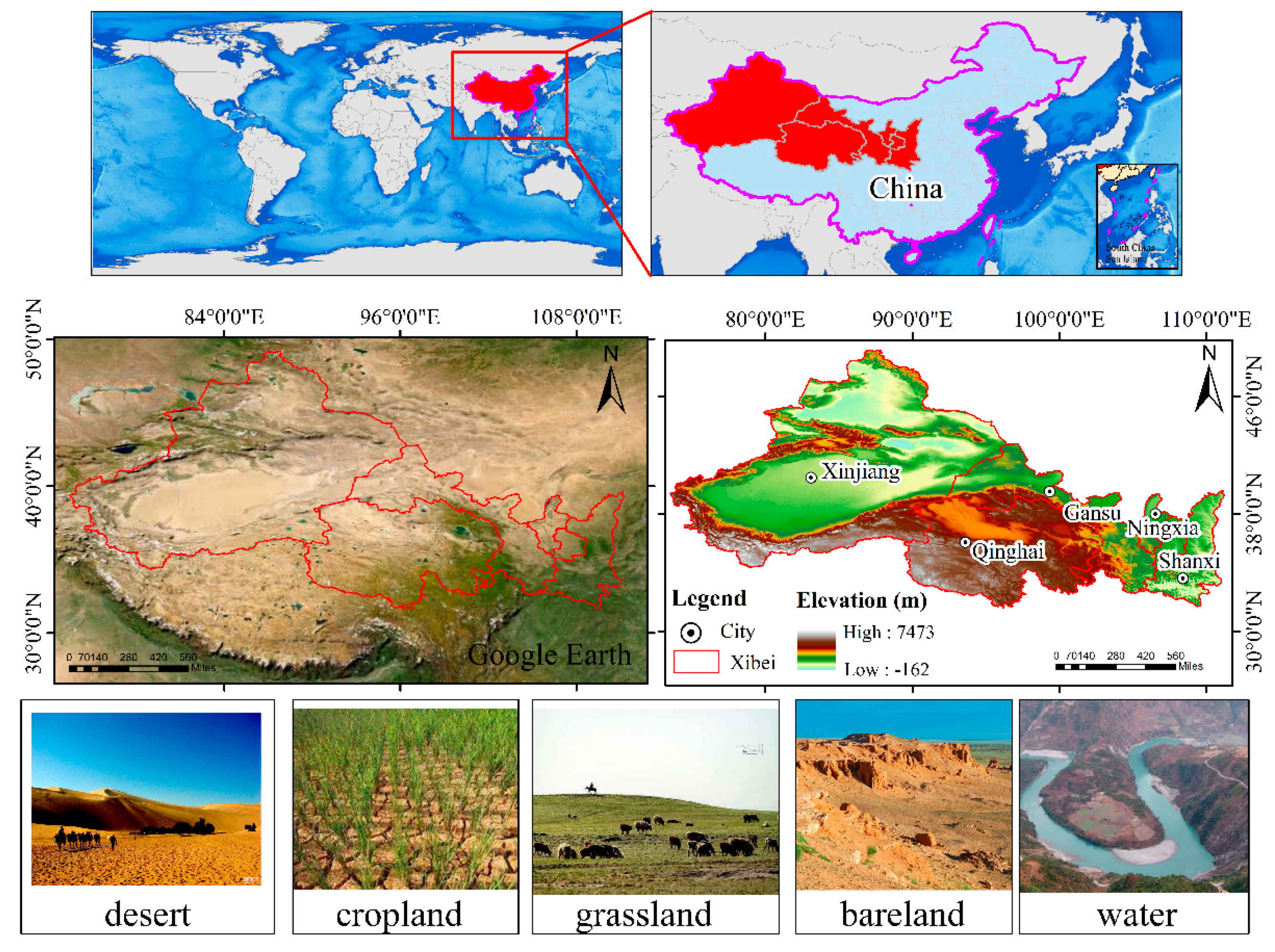
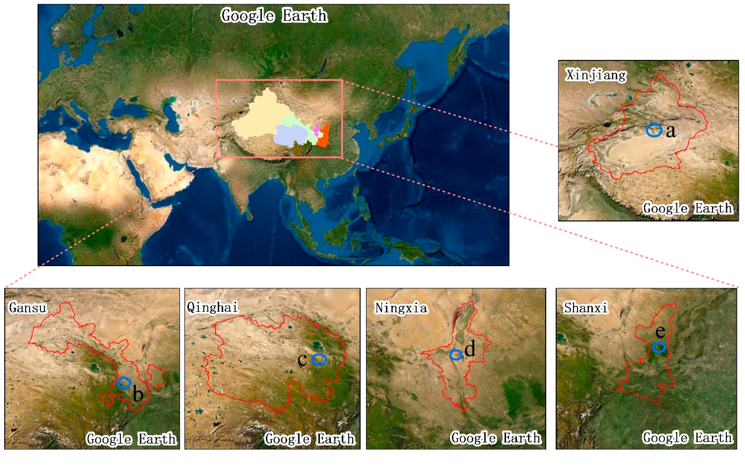
2.1. Study Area

The study area is located in the northwestern region of China’s seven geographical regions (Figure 1). The study area includes Xinjiang, Gansu, Qinghai, Ningxia, and Shaanxi provinces. The neighboring countries include Mongolia, Russia, Kazakhstan, Kyrgyzstan, Tajikistan, Afghanistan, Pakistan, and India. Northwestern China covers a vast area characterized by alternating mountains, plateaus, and basins, with complex and varied landforms and huge differences. The study area has a large north–south span, a complex geographical environment, and diverse ecological conditions, so there is a wide variety of wild animals and plants. Northwestern China is characterized by poor natural conditions, an extremely fragile ecological environment, sparse vegetation, and limited water vapor evaporation from the ground. The annual precipitation in northwestern China is generally larger in the east and smaller in the west, and it decreases from about 400 mm in the east to 200 mm, or even less than 50 mm, in the west. The rivers in this region are mainly internal rivers, and the water supply is mainly from precipitation in the mountainous areas and snow melt water. Drought is the main natural feature of northwestern China and is one of the main reasons for its relatively fragile ecological environment. Northwestern China has a long border and is China’s gateway to the west. It plays a very important role in China’s political, national defense, and ecological security. Most of the study area has a continental climate and is located in the mid-temperate zone and warm temperate zone, but some areas have an alpine climate. The overall distribution of the annual average temperature is lower in the north than in the south, and lower in the mountainous areas than on the plains.

2.2. Data and Preprocessing

In this study, three high-resolution land cover products that are currently freely published were selected for evaluation and analysis. The three products are the Finer Resolution Observation and Monitoring of Global Land Cover (FROM-GLC) product (http://data.ess.tsinghua.edu.cn./, accessed on 6 January 2022) produced by Tsinghua University [38], the ESA product (https://zenodo.org/record/5571936, accessed on 8 January 2022) produced by the European Space Agency, and the ESRI product (https://www.arcgis.com/index.html, accessed on 2 January 2022) produced by the Environmental Systems Research Institute [39] (

Table 1. The main parameters of the three land cover products.

Name	Resolution (m)	Number of Categories	Time	Method	Overall Accuracy (%)	Producer	Satellite
FROM-GLC	10	10	2017	Random forest	72.76	Tsinghua University	Sentinel-2
ESA	10	11	2020	Deep learning model	74.40	European Space Agency	Sentinel-1/2
ESRI	10	10	2020	Deep learning model	85.96	Impact Observatory for ESRI	Sentinel-2

). Although the time periods of the products selected for use in this study vary, natural ecosystems usually change significantly over a period of 10 years or more [40]. In addition, it was verified using a Google Earth high-resolution image that the ecological status of the study area was in a relatively stable state during this period, so the selected data satisfactorily support this research.

The original data was preprocessed before the data evaluation and analysis. This processing mainly included data cutting, projection transformation, unification of the resolution, and the unification of the classification systems among the different products. First, the ArcGIS software was used to cut the three land cover data products using the vector boundary of the northwestern region. Second, the coordinates of all of the land cover data were unified to the UTM projection and WGS84 coordinate system. Finally, the unification of classification systems took place. In the comparative evaluation of the different land cover products, the classification systems needed to be merged under the same classification benchmarks [41] to reduce errors. According to previous studies [42,43] and the definitions of tundra, moss, and lichen, the types of tundra in the FROM-GLC product and moss and lichen in the ESA product were merged into shrubland. In addition, the proportion of the cloud cover pixels in the ESRI product to the total pixels in the study area was very small, and thus was ignored.

Table 2. The merged classification system and its correspondence with the original classification systems.

Merged	Code	FROM-GLC	Code	ESA	Code	ESRI
Cropland	10	Cropland	40	Cropland	5	Crops
Forest	20	Forest	10	Tree cover	2	Trees
Grassland	30	Grassland	30	Grassland	3	Grass
Shrubland	40	Shrubland	20	Shrubland	6	Scrub
	70	Tundra	100	Moss and Lichen
Wetland	50	Wetland	90	Herbaceous wetland	4	Flooded vegetation
			95	Mangroves
Water	60	Water	80	Permanent water bodies	1	Water
Built-up	80	Impervious surfaces	50	Built-up	7	Built-up area
Bare land	90	Bare land	60	Bare/sparse vegetation	8	Bare ground
Snow/Ice	100	Snow/Ice	70	Snow and Ice	9	Snow/Ice

presents the classification system for the three land cover products, and Figure 2 shows the three land cover products after preprocessing.

3. Methods

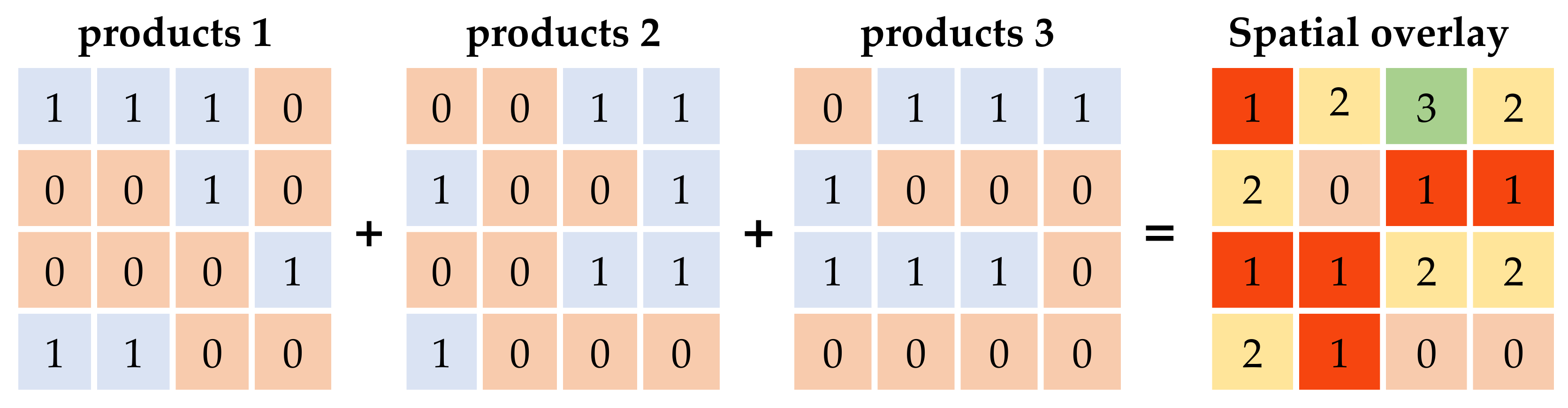
3.1. Constituent Similarity Evaluation

For each land cover product, the area of each land cover type was summarized individually, and the correlation calculation was carried out for the corresponding area sequence of the land cover types between the different datasets in order to evaluate the similarities of the land compositions of each land cover type among the products [44]. The calculation formula is as follows:

$$R_i=\frac{{{\displaystyle \sum }}_{i=1}^n\left(X_i-\overline{X}\right)\left(Y_i-\overline{Y}\right)}{\sqrt{{{\displaystyle \sum }}_{i=1}^n{\left(X_i-\overline{X}\right)}^2{{\displaystyle \sum }}_{i=1}^n{\left(Y_i-\overline{Y}\right)}^2}}$$

(1)

where $R_i$ is the area correlation coefficient; $i$ is the land cover type; $X_i$ is the total area (km²) of type $i$ in dataset $X$; $Y_i$ is the total area (km²) of type $i$ in dataset $Y$; $\overline{X}$ is the average (km²) of the total area of all of the types in dataset $X$; $\overline{Y}$ is the average (km²) of the total area of all of the types in dataset $Y$; and $n$ is the total number of land cover types.

3.2. Evaluation of Spatial Distributions

To intuitively express the consistency of the spatial distributions of the three land cover products in this study, based on the spatial superposition of the three datasets, which was conducted in ArcGIS, the calculation results were summarized into three situations: ① completely inconsistent: the three datasets exhibit completely different land cover categories within a given pixel; ② basically consistent: there are only two types of land cover in a corresponding given pixel for the three datasets; and ③ Completely consistent: the three datasets have exactly the same land cover type in a given pixel [44]. Taking forests as an example, a schematic diagram of the spatial overlay is shown in Figure 3.

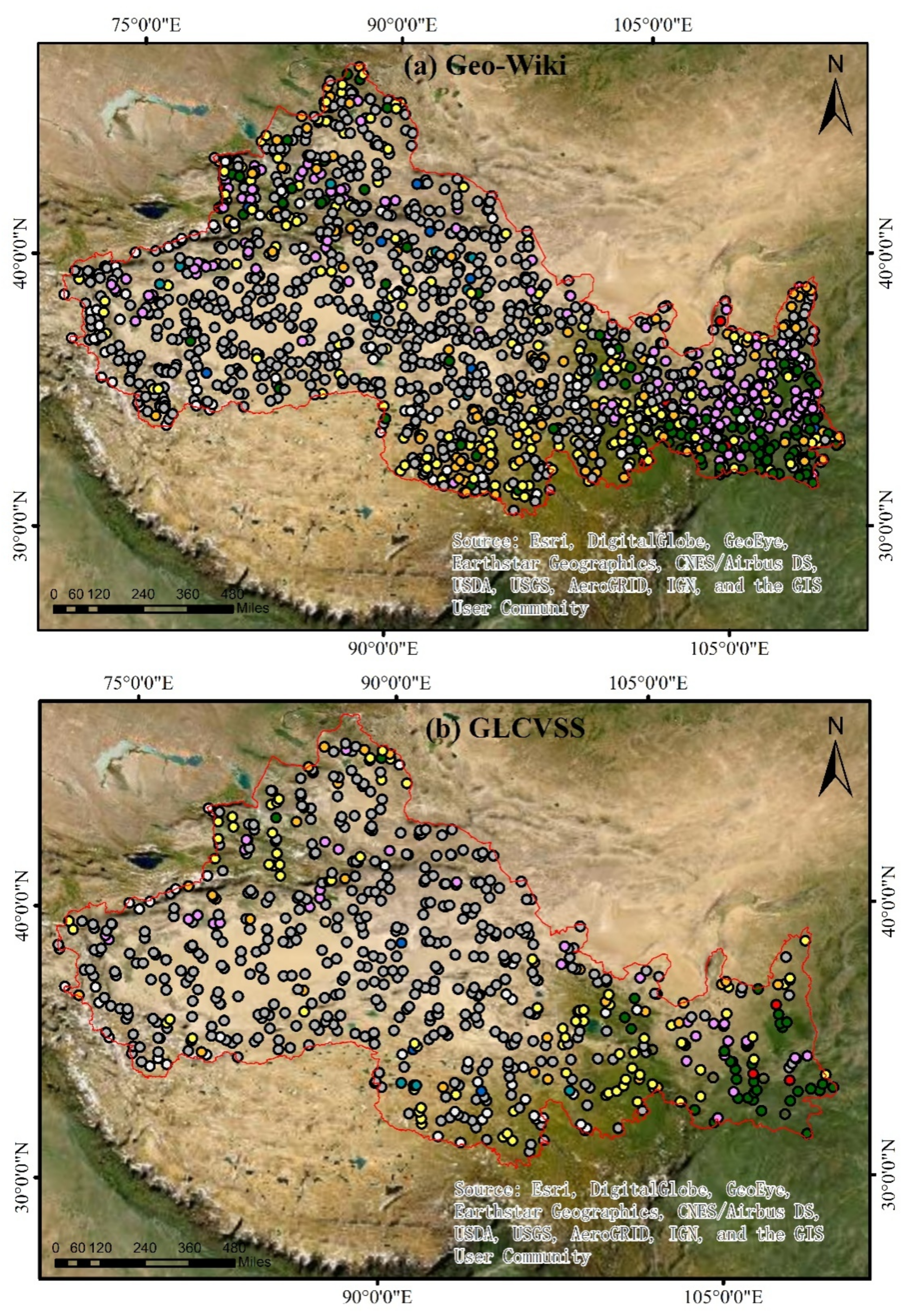
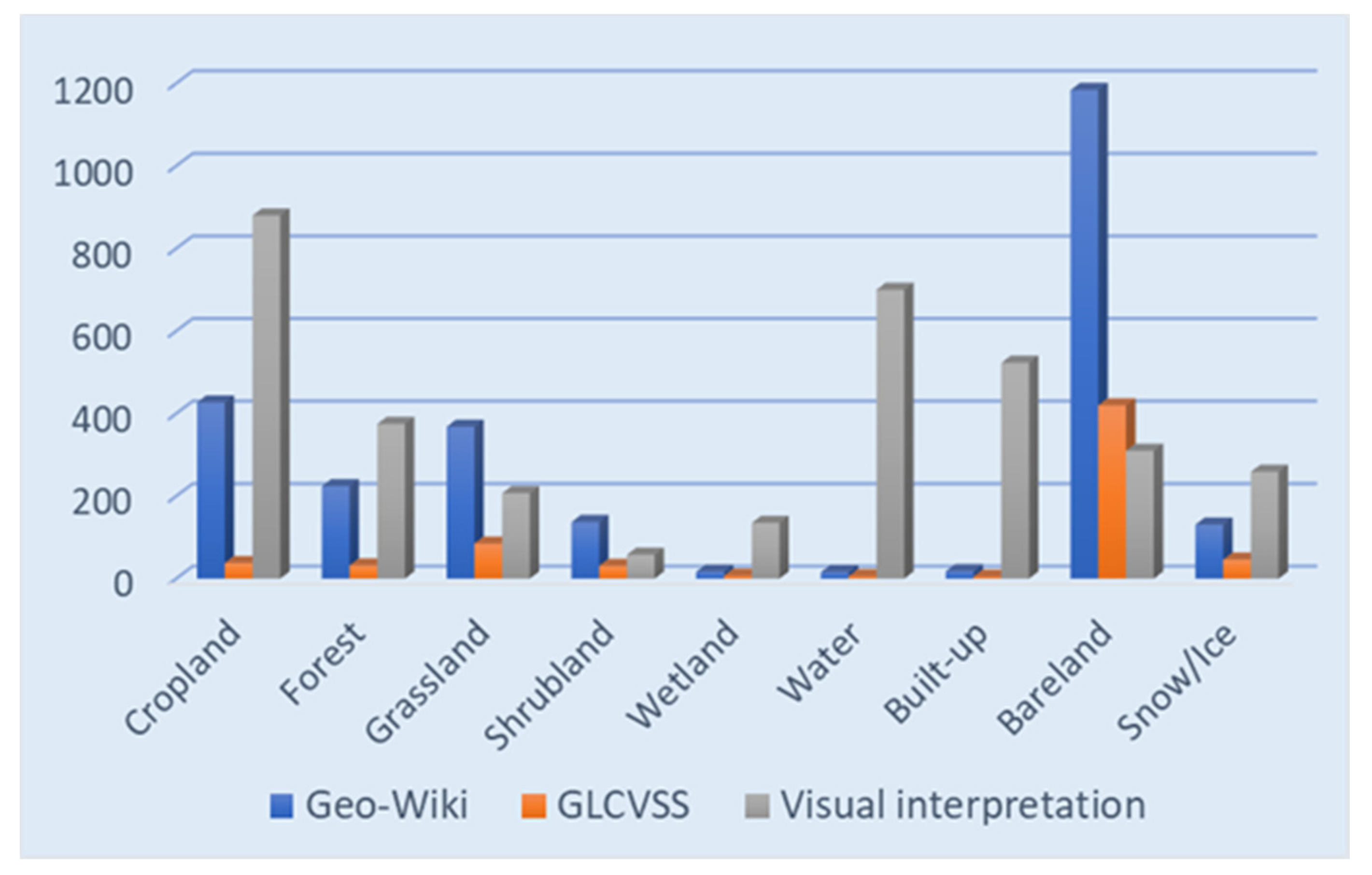
3.3. Sample Accuracy Evaluation

The error matrix is a method that is commonly used in the accuracy evaluation of land cover data [45,46]. This method mainly compares the category consistency of the reference data and the data to be verified at a specific location, and then it establishes the error matrix between them. The overall accuracy (OA), producer accuracy (PA), user accuracy (UA), and kappa coefficients are calculated to express the accuracy of the data to be verified. The calculation formulas of these indexes [47] are as follows:

$$\mathrm{OA}=\frac{{{\displaystyle \sum }}_{i=1}^r{x}_{ii}}{n^2}\times 100\%$$

(2)

$$\mathrm{PA}=\frac{x_{ii}}{x_{+i}}\times 100\%$$

(3)

$$\mathrm{UA}=\frac{x_{ii}}{x_{i+}}\times 100\%$$

(4)

$$\mathrm{Kappa}=\frac{N·{{\displaystyle \sum }}_{i=1}^r{x}_{ii}-{{\displaystyle \sum }}_{i=1}^r\left(x_{i+}·x_{+i}\right)}{N^2-{{\displaystyle \sum }}_{i=1}^r\left(x_{i+}·x_{+i}\right)}$$

(5)

where $x_{ii}$ is the correctly classified number of pixels for land cover type $i$; $n$ is the total number of pixels; $x_{i+}$ is the total number of pixels containing land cover type $i$ in the data to be verified; $x_{+i}$ is the total number of pixels containing land cover type $i$ in the reference data; $r$ is the number of rows in the confusion matrix; and $N$ is the total number of samples.

It is important to have a sufficient number of accurate validation samples in land cover mapping and its accuracy evaluation. In the validation of large-scale land cover datasets, ground reference data are difficult to obtain. Therefore, a common global validation dataset, especially one that is adequate, well described, compatible, and updated in real time, would greatly facilitate the assessment of land cover data. Several studies have demonstrated the potential of using third-party validation data in land cover evaluation [48,49]. For example, Foody used two sources of volunteered data to illustrate the potential of using amateur or neogeographical activity in map validation [50]. Therefore, in order to compare and evaluate the accuracies of the three land cover products, three independent validation sample sets were used in this study: (1) The Geo-Wiki samples from four separate campaigns [51] were obtained from the Geo-Wiki (http://geo-wiki.org/, accessed on 15 January 2022) crowdsourcing platform, including a total of 10 land cover types. The Geo-Wiki datasets described information on human impacts, land cover disagreement, wilderness, and reference data. These data have been made available to the scientific community for use as reference data for global satellite-derived products, as well as for monitoring global terrestrial ecosystems in general. After processing the Geo-Wiki global validation samples, 2522 validation samples covering the study area were obtained (Figure 4a). (2) The Global Land Cover Validation Sample Set (GLCVSS) [52] follows a random sampling strategy to ensure that all of the samples are evenly distributed across the globe. The GLCVSS samples are based on the interpretation of Landsat Thematic Mapper (TM) images, Enhanced Thematic Mapper Plus (ETM+) images, and the MODIS Enhanced Vegetation Index (EVI) time series data and were supplemented by other high-resolution imagery from Google Earth. This records the quality of the reference data and the confidence of the interpreter. After processing the GLCVSS global samples, 670 validation samples covering the study area were obtained (Figure 4b). (3) The validation samples were obtained via visual interpretation. Google Earth is one of the main data sources for images used for accuracy evaluation due to its accurate positioning, rich temporal phase, high resolution, easy access, and wide overlay of these images [46,53]. In order to reduce the negative impact of positioning and interpretation errors on the sample quality, the following principles were followed when selecting and interpreting samples: first, in order to reduce the effect of the positioning error, the sample point was selected in the center of a homogeneous region. Second, in order to reduce the interpretation errors caused by the temporal phase of the data, remote sensing images from 2017 to 2020, which were consistent with the temporal phase of the data to be evaluated, were mainly used. Third, for some of the more difficult to interpret samples, the interpretation was assisted by combining references with other information, such as using the voluntary geo-information platform (Geo-wiki) [54] to assist in the interpretation. Fourth, multiple independent interpretations were used, and a sample was discarded when the interpretation results did not agree after negotiation. Based on Google Earth images, Sentinel images, and the aforementioned two third-party validation samples, 3447 validation samples covering the study area were finally obtained through visual interpretation (Figure 4c). Figure 5 shows the number of samples of each type for the three independent validation samples.

4. Results

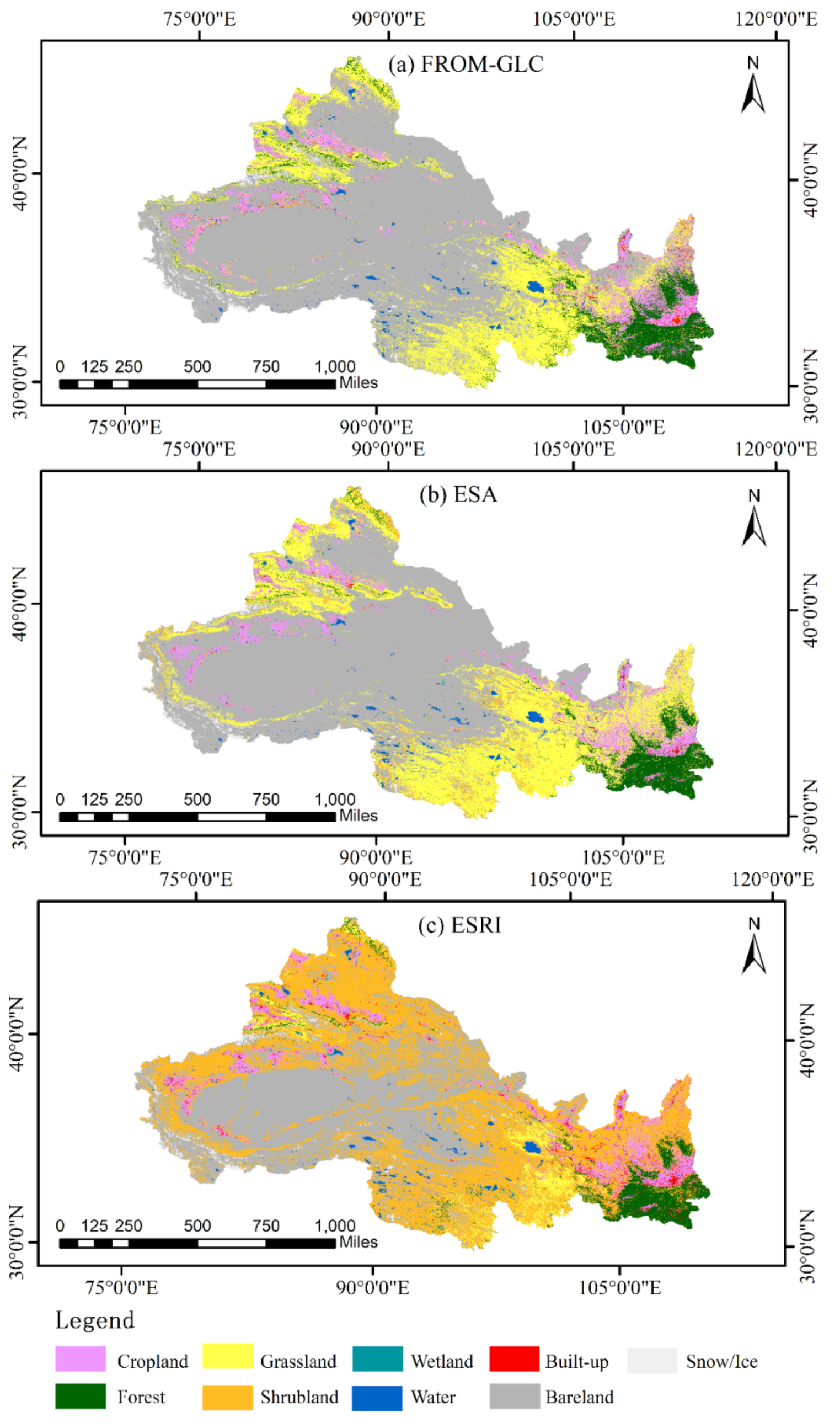
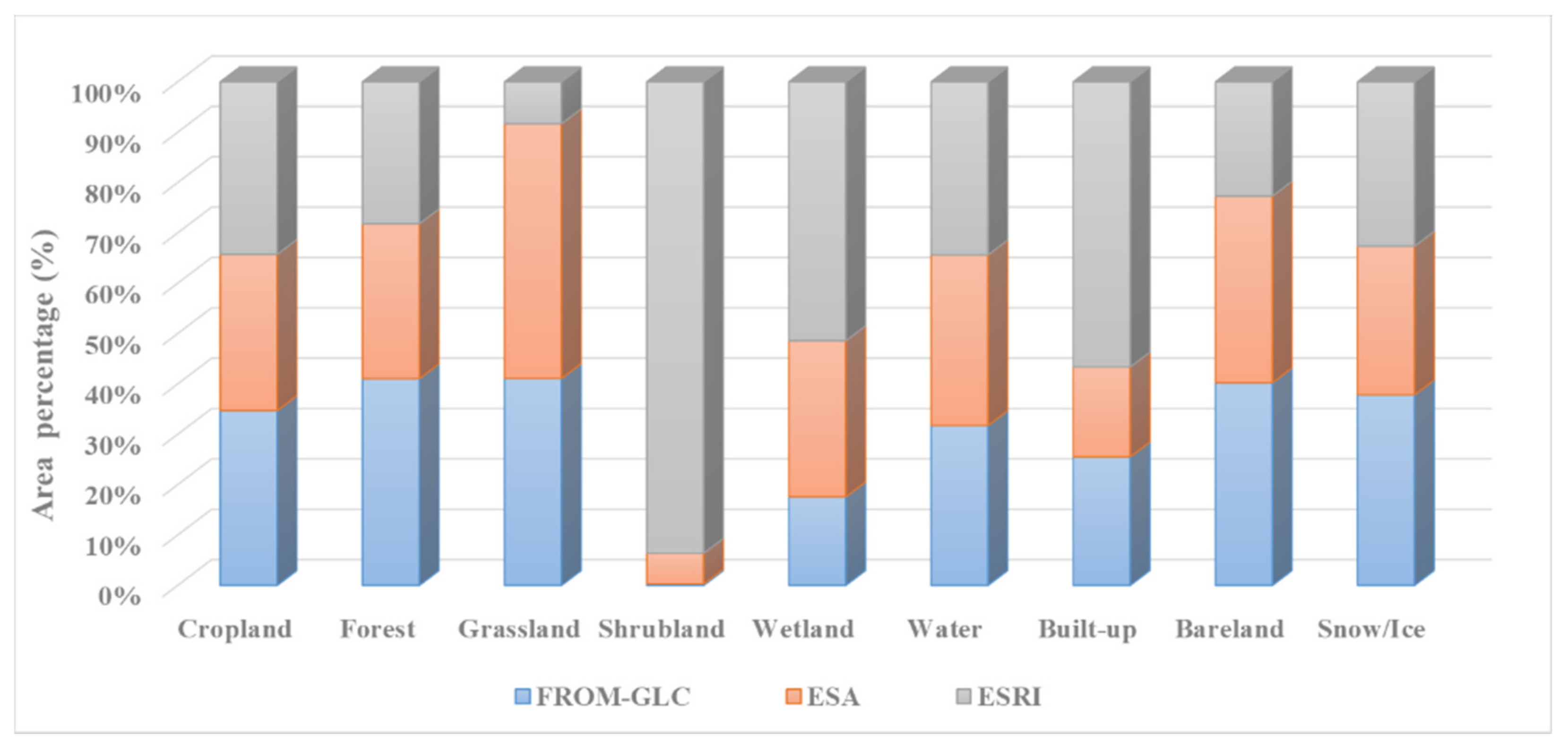
4.1. Comparative Analysis of Land Cover Composition

Figure 6 shows the results of the comparison of the area compositions of the three land cover products. The experimental results show that the consistencies for the cropland, forest, water bodies, and snow/ice areas of the three products were relatively high. The consistencies for the grassland, built-up land, and bare land areas of the FROM-GLC and ESA products were higher. The percentages of grassland, built-up land, and bare land for the FROM-GLC product were 21.19%, 0.74%, and 61.85%, respectively. The percentages of grassland, built-up land, and bare land for the ESA product were 26.07%, 0.52%, and 56.97%, respectively. The shrubland and wetland areas of the three products were uniformly low, especially the shrubland, and the percentages of the shrubland in the study area were 0.13% for the FROM-GLC, 2.96% for the ESA, and 45.32% for the ESRI.

By calculating the area correlation coefficient between the three products, it was found that the area correlation coefficient between the FROM-GLC and ESA products was the highest (0.99), indicating that these two products had a relatively high similarity in terms of the land cover types in the study area. The ESA and ESRI products had the next highest similarity, with an area correlation coefficient of 0.47. The area correlation coefficient between the FROM-GLC and ESRI was the lowest (0.45).

4.2. Analysis of Spatial Distribution Differences

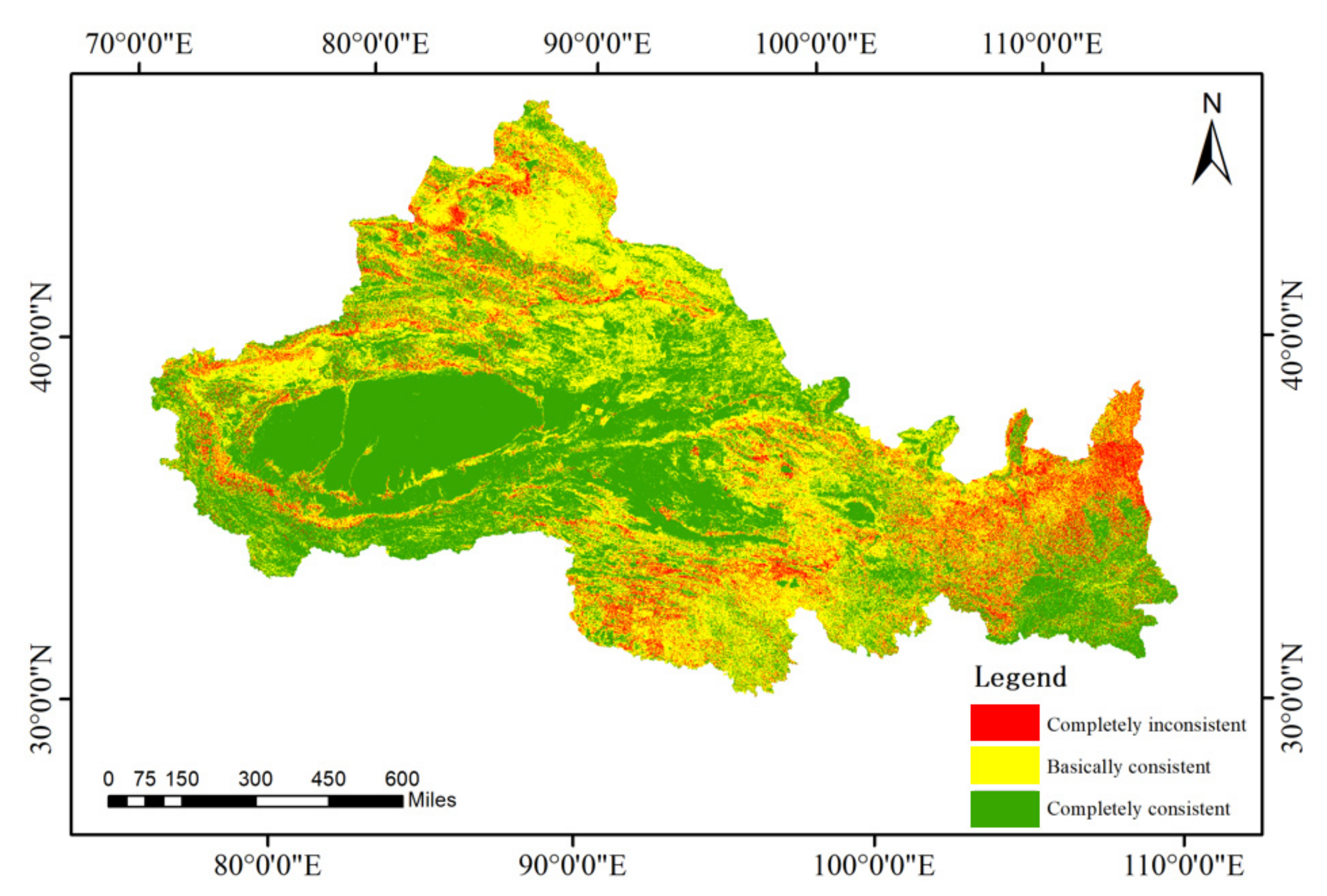
4.2.1. Consistency of Spatial Distribution

Figure 7 shows the consistency of the spatial distributions of the three products obtained using the spatial superposition method. The results show that the completely consistent areas of the three products were mainly distributed in the western part of the study area, and fewer completely consistent areas were located in the central and eastern parts of the study area. The land cover types in these areas were singular, mainly bare land and forest. The completely consistent areas accounted for 46.26% of the total area of the study area. The basically consistent areas of the three products were mainly distributed in the northern part of the study area, and fewer completely consistent areas were located in the eastern and southern parts of the study area. The land cover types in these areas were more complex, and the land surface spatial heterogeneity was higher. The basically consistent areas accounted for 42.77% of the total area of the study area. The completely inconsistent areas of the three products were mainly distributed in the eastern and southern parts of the study area, and fewer completely inconsistent areas were located in the northern part of the study area. The land cover types in these areas were cross-distributed (e.g., cropland, forest, and grassland), and the spatial heterogeneity of the surface was high. The completely inconsistent areas accounted for 10.97% of the total area of the study area.

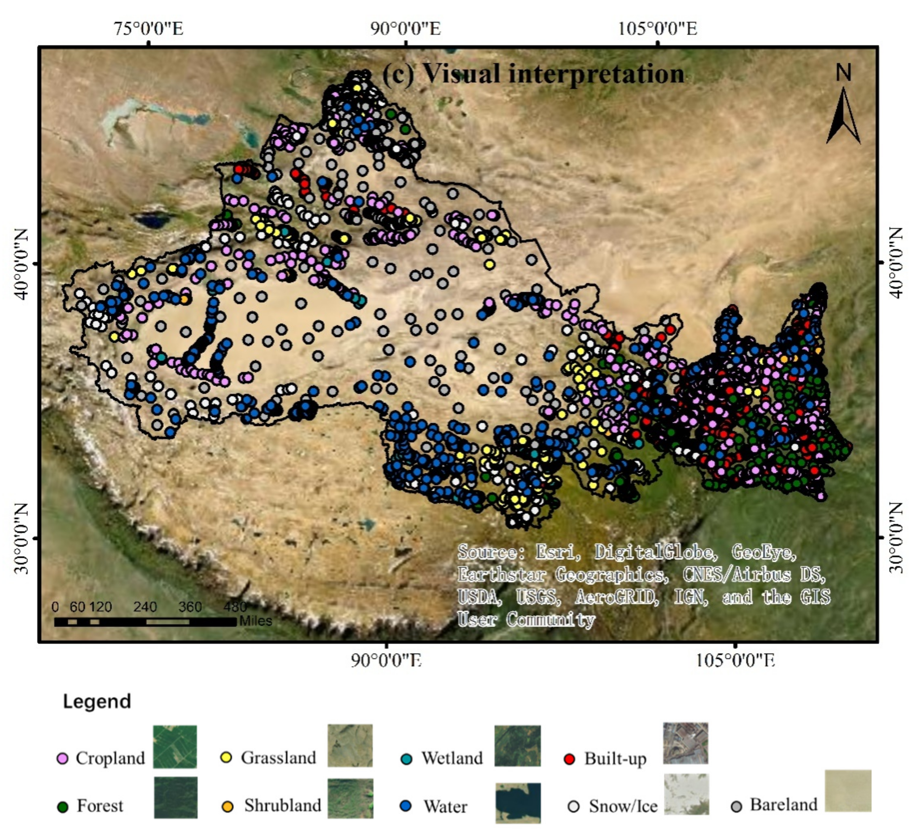
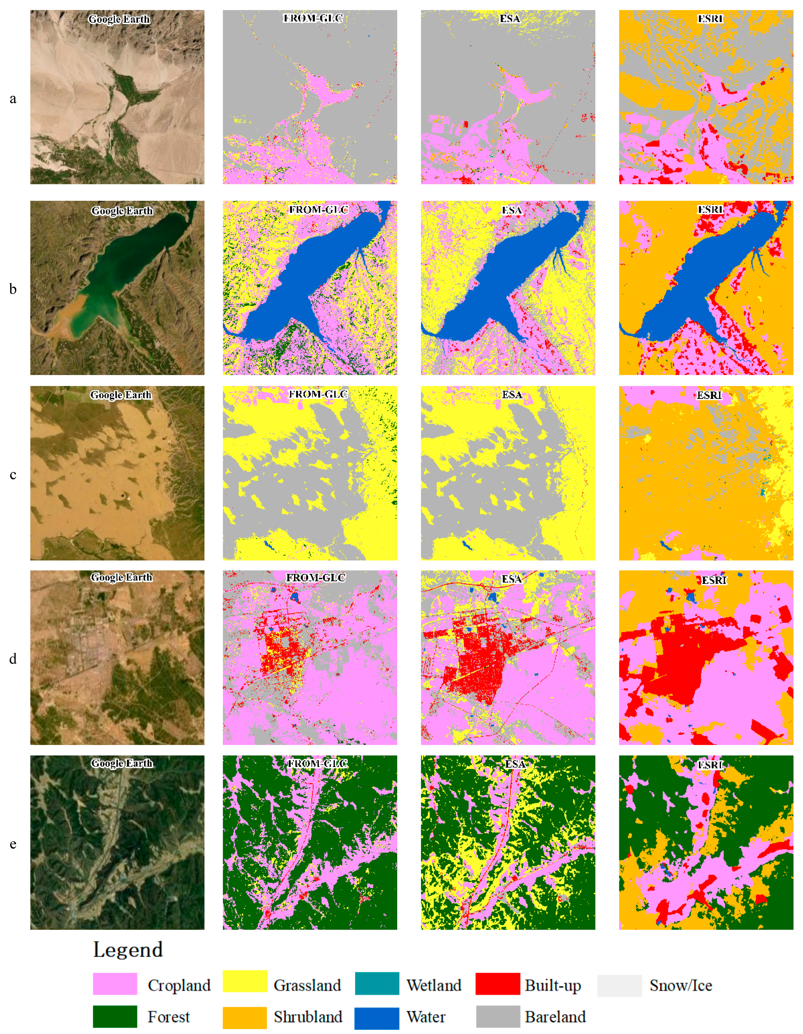
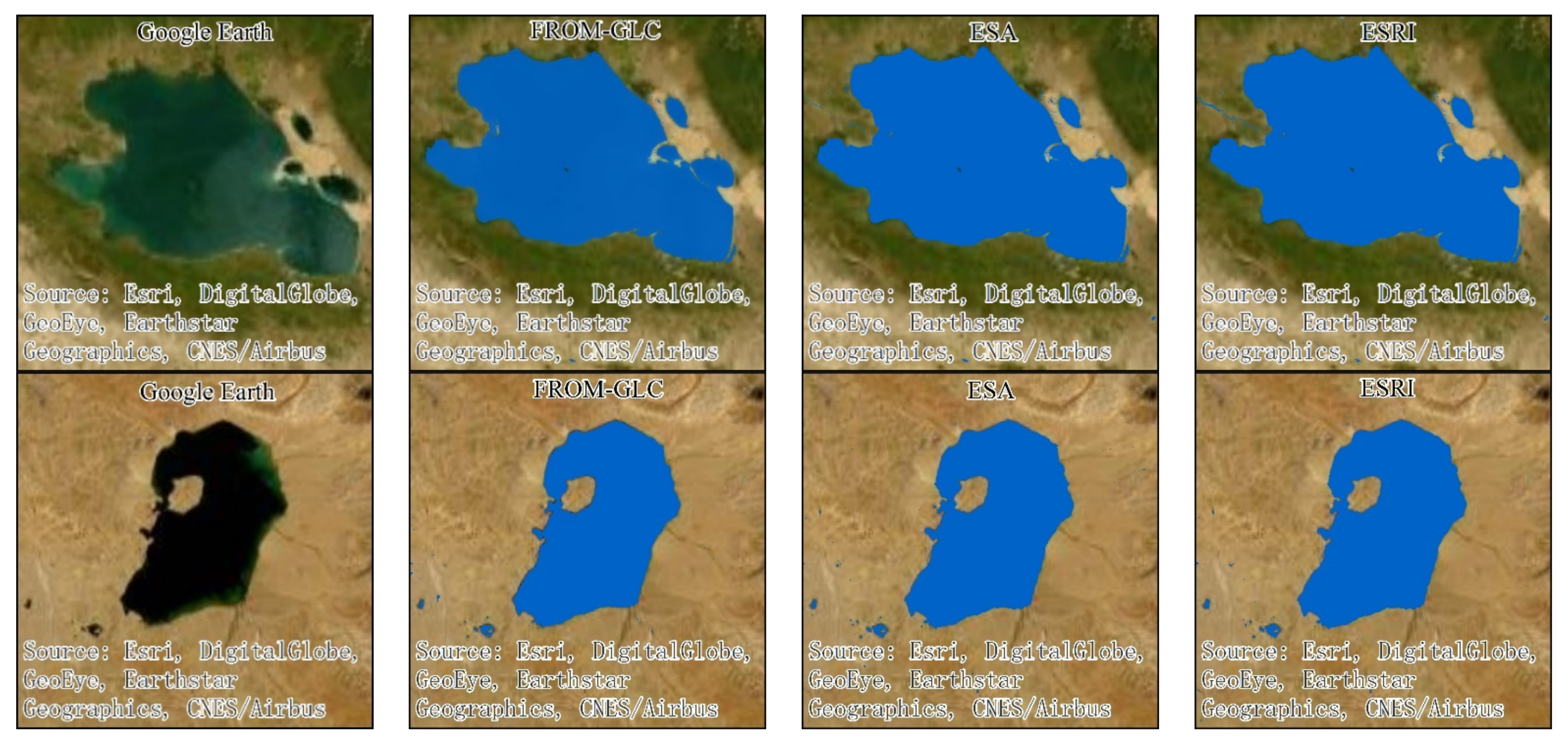
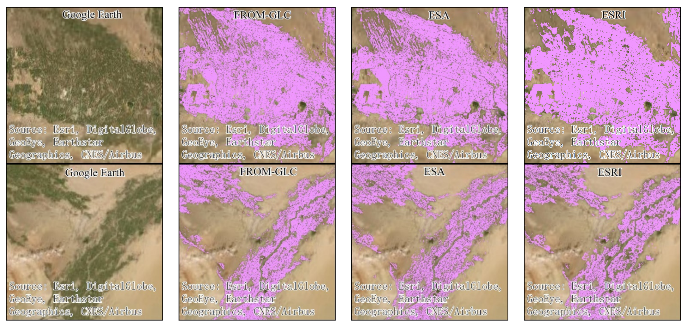
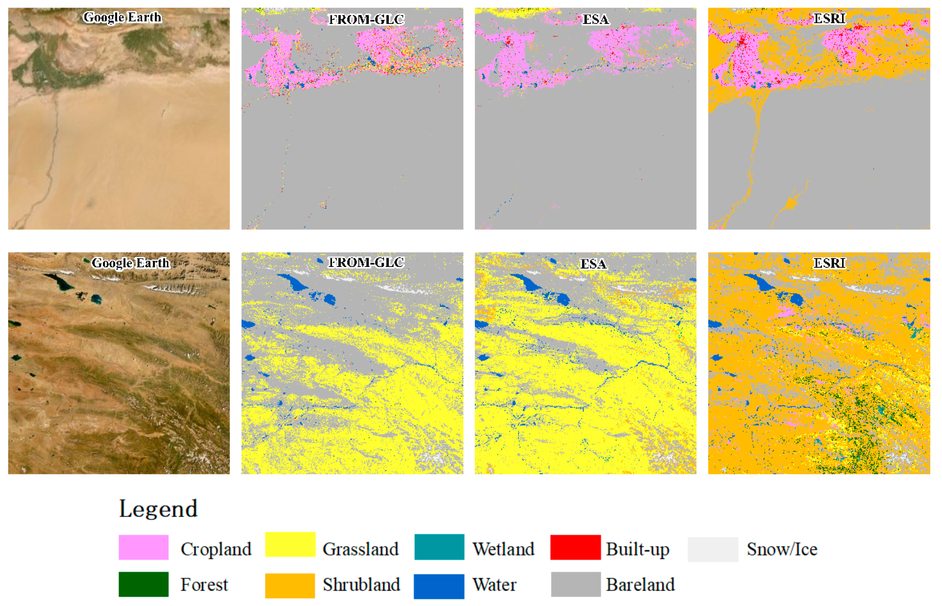
4.2.2. Comparative Analysis Using Google Earth Images

Based on high-resolution Google Earth images, the different land cover types were selected in the five provinces in the study area to verify the accuracy of the three land cover products and to compare the consistency of the spatial distributions of the three products (Figure 8). As can be seen from area a in Figure 8, the FROM-GLC and ESA products had a high accuracy and spatial consistency. The spatial distributions of the cropland and bare land for the two products were basically the same. The low accuracy of the ESRI product was mainly due to the serious confusion between shrubland and bare land, which also led to the low consistency of the ESRI product with the other two products. It can be seen from area b in Figure 8 that the water bodies of the three products had a high accuracy and consistency. The accuracy of the FROM-GLC and ESA products for the other land cover types was slightly lower, mainly due to the serious confusion between the cropland and grassland. The accuracy for other land cover types for the ESRI product was low, mainly due to the serious confusion between cropland and shrubland. It can be seen from area c in Figure 8 that the FROM-GLC and ESA products had a higher accuracy for bare land, but a lower accuracy for the other land cover types. The main reason for this is that the FROM-GLC and ESA products classified part of the cropland as grassland. The accuracy of the ESRI products was low, mainly due to the misclassification of bare land as shrubland. It can be seen from area d in Figure 8 that the accuracy for cropland of the three products was high, followed by that for built-up land, and the accuracies for the other land cover types were low. This is mainly because it is difficult to accurately distinguish between bare land, grassland, and shrubland. As can be seen from area e in Figure 8, the accuracy for cropland of the three products was high, followed by forest and built-up land, and the accuracies for the other land cover types were low. This is mainly because it is difficult to accurately distinguish between forest, grassland, and shrubland.

4.3. Absolute Accuracy Evaluation

Table 3. Accuracy evaluation results based on Geo-Wiki samples.

Geo-Wiki
		1	2	3	4	5	6	7	8	9	OA (%)	Kappa
FROM-GLC	PA (%)	61.59	63.39	47.55	0.00	0.00	18.75	27.78	62.67	20.61	53.81	0.37
	UA (%)	75.79	47.33	24.31	0.00	0.00	30.00	5.75	72.60	79.41
ESA	PA (%)	47.54	58.03	56.52	6.57	0.00	18.75	16.67	56.08	16.03	49.21	0.32
	UA (%)	84.23	57.27	21.03	12.33	0.00	27.27	15.00	71.10	84.00
ESRI	PA (%)	49.18	57.59	12.50	58.39	0.00	25.00	66.67	34.40	12.98	35.90	0.24
	UA (%)	80.15	58.90	37.71	6.27	0.00	40.00	17.14	77.23	58.62

Note: 1—Cropland; 2—Forest; 3—Grassland; 4—Shrubland; 5—Wetland; 6—Water bodies; 7—Built-up land; 8—Bare land; 9—Snow/Ice.

presents the accuracy evaluation results for the three land cover products based on the Geo-Wiki verification samples. The results show that the FROM-GLC product had the highest OA and kappa values (53.81% and 0.37, respectively), followed by the ESA product, with OA and kappa values of 49.21% and 0.32, respectively. The OA (35.90%) and kappa (0.24) values of the ESRI product were the lowest among the three products. For the accuracy for the nine surface types in the study area, the three products all had low PA and UA values for shrubland and wetland, indicating that serious misclassification and omission of these two types occurred. The FROM-GLC product had high PA and UA values for cropland and bare land, a high PA value for forest, a high UA value for snow/ice, and low PA and UA values for the other land cover types. The ESA product had high UA values for cropland, bare land, and snow/ice, and low PA and UA values for the other land cover types. For the ESRI product, the cropland and bare land had high UA values, the built-up land had a high PA value, and the other land cover types had low PA and UA values.

Table 4. Accuracy evaluation results based on GLCVSS samples.

GLCVSS
		1	2	3	4	5	6	7	8	9	OA (%)	Kappa
FROM-GLC	PA (%)	65.79	75.00	68.24	0.00	0.00	33.33	0.00	87.62	23.91	73.45	0.52
	UA (%)	58.14	66.67	41.14	0.00	0.00	25.00	0.00	86.59	100.00
ESA	PA (%)	57.90	68.75	76.47	6.45	0.00	0.00	50.00	84.29	17.39	71.64	0.51
	UA (%)	68.75	91.67	39.63	8.00	0.00	0.00	66.67	87.62	100.00
ESRI	PA (%)	73.68	68.75	21.18	80.65	25.00	0.00	50.00	53.81	17.39	49.78	0.31
	UA (%)	68.29	81.48	66.67	8.28	100.00	0.00	33.33	91.50	88.89

Note: 1—Cropland; 2—Forest; 3—Grassland; 4—Shrubland; 5—Wetland; 6—Water bodies; 7—Built-up land; 8—Bare land; 9—Snow/Ice.

presents the accuracy evaluation results for the three land cover products based on the GLCVSS validation samples. The results show that the FROM-GLC and ESA products had higher OA values (73.45% and 71.64%, respectively). The ESRI product had lower OA and kappa values (49.78% and 0.31, respectively). Regarding the precision of each land cover type, for the FROM-GLC product, shrubland, wetland, and built-up land had lower PA and UA values. For the ESA product, the PA and UA values of wetland and water bodies were lower. For the ESRI product, the PA and UA values of water bodies were lower.

Table 5. Accuracy evaluation results based on the visual interpretation samples.

Visual interpretation
		1	2	3	4	5	6	7	8	9	OA (%)	Kappa
FROM-GLC	PA (%)	74.53	88.45	79.23	1.72	4.44	70.10	62.09	79.43	40.54	67.03	0.62
	UA (%)	83.93	85.10	25.31	20.00	28.57	98.79	89.73	39.89	99.06
ESA	PA (%)	74.66	63.73	85.02	5.17	13.33	74.96	77.63	61.29	31.66	66.60	0.61
	UA (%)	96.33	88.19	23.78	3.00	75.00	99.62	97.60	31.41	100.00
ESRI	PA (%)	68.52	57.60	33.33	77.59	34.07	76.11	98.66	26.13	39.77	64.16	0.59
	UA (%)	95.87	91.14	46.94	4.81	95.83	99.25	88.81	35.53	99.04

Note: 1—Cropland; 2—Forest; 3—Grassland; 4—Shrubland; 5—Wetland; 6—Water bodies; 7—Built-up land; 8—Bare land; 9—Snow/Ice.

presents the accuracy evaluation results for the three land cover products based on the visual interpretation validation samples. The results show that the OA values of the three products were all greater than 60%, and the OA and kappa values of the FROM-GLC product, 67.03% and 0.62, respectively, were the highest among the three datasets. Regarding the precision for each type of land cover, for the FROM-GLC product, the PA and UA values of shrubland and wetland were lower. For the ESA product, the PA and UA values of shrubland were lower, the PA value of wetland was lower, and the UA value of grassland was lower. For the ESRI product, the UA value of shrubland was lower.

To conclude, the accuracy evaluation results for the three validation samples all demonstrate that the FROM-GLC product had the highest OA value, followed by the ESA product, and the ESRI product had the lowest OA value. Regarding the accuracies for the nine land cover types, for all three products, the accuracies for shrubland and wetland were lower, indicating that the misclassification and omission of these two land cover types were more serious and their accuracies need to be improved further.

5. Discussion

5.1. Analysis of the Influence of Typical Land Cover Type Differences on Research in Drought Regions

Water is the lifeblood of ecosystems in drought regions, and improving the ecosystems and ecological construction are the primary problems to be solved in development and construction in western China [55]. Therefore, the distribution, development, and utilization of water resources in northwestern China are of great strategic significance to the formation of a new pattern of regional development. In this study, it was found that the FROM-GLC, ESA, and ESRI products had a high consistency for water bodies, with area percentages of 1.02%, 1.08%, and 1.10%, respectively. The three products had better abilities to depict the boundary contours of water bodies (Figure 9). The UA values of the FROM-GLC, ESA, and ESRI were 98.79%, 99.62%, and 99.25%, respectively, based on the accuracy evaluation of the visual interpretation verification samples. Therefore, the FROM-GLC, ESA, and ESRI products can provide supporting data for water-related research in drought regions. For example, for water resource carrying capacity evaluations in drought areas, the area covered by water bodies is an important factor in model calculations—if the extraction of the water body area is not accurate, this will affect the water resource yield and total water resources calculations in the water resource carrying capacity model, and thus it will affect the calculation of water resource carrying capacity [55].

Cropland is the core resource for agricultural production and is a strategic resource related to food production. Its situation is related to the security of global food production and the stability of the social economy [56]. Continuous population growth leads to rapid growth of the demand for food consumption, and the contradiction between the demand for cropland resources and its own scarcity and finiteness is increasing. In particular, in northwestern China, where the utilization of cropland resources is more serious, this issue has received widespread attention from all sectors of society [57]. The ecological functions in the drought region in northwestern China are extremely important in China and globally. The expression ability of the boundary contour of the cropland resources for the three land cover products is good (Figure 10). In this study, the UA values of the FROM-GLC, ESA, and ESRI products were found to be 83.93%, 96.33%, and 95.87%, respectively, based on the accuracy evaluation using the visual interpretation verification samples. Therefore, the three products can provide auxiliary data for related research on cropland resources. For example, the statistical data for the cropland areas are a key factor in the evaluation of cropland productivity in drought regions. If the accuracy of the cropland cover data is low, the calculation of the multiple cropping indexes and yield per unit area of the sown cropland area in the cropland productivity model will be affected, and, thus, the final evaluation results will be affected.

In northwestern China, the geological environment is complex and precipitation is scarce. Most of the areas are desert (Gobi), underlying sparse vegetation, and climate change has been very drastic [58]. In northwestern China, vegetation changes have had significant effects on surface temperature, precipitation, and surface energy, and even on the intensity of the east Asian summer monsoon [59]. In addition, the impact of vegetation changes on hydrological processes plays a very important role in the growth and maintenance of the vegetation itself, especially in northwestern China, where water resources are relatively scarce and the ecological environment is relatively fragile. Therefore, it is important to monitor the spatial distribution of (and changes in) the vegetation in northwestern China for a long time. In this study, the accuracies for the vegetation types of the FROM-GLC, ESA, and ESRI land cover products covering northwestern China were found to be low, and there were large differences between the products, especially for grassland, shrubland, and wetland. Therefore, in order to provide data support for studies on the impact of vegetation changes on regional climates, regional surface hydrological variables (e.g., precipitation), and regional soil and water loss monitoring, the accuracy for the vegetation types of the three land cover products should be improved.

5.2. Discussion of Inconsistent Factors

The dataset development rules (such as classification system and classification method), established by different production organizations, can lead to differences between products, posing great challenges to the strict comparison of maps and the collaborative use of different maps [60].

The differences in some of the subordinate definitions of the land cover types in the classification systems are one of the factors contributing to the low spatial consistency between the FROM-GLC, ESA, and ESRI products. The global scale land cover classification system is mainly used for global classification and considers the characteristics of the global land cover information, which inevitably affects its analysis and application in local areas [44].

In this study, it was found that the main reason for the low consistency between the FROM-GLC, ESA, and ESRI products was that the three products had great differences in their discrimination between grassland, shrubland, and bare land (Figure 11), and especially between grassland and shrubland. However, sparse vegetation, shrubland, and other vegetation types have high semantic similarities. Therefore, for the extraction of several vegetation types, the unified vegetation coverage and tree height factor values should be clearly stated when establishing the classification system to reduce the uncertainty caused by the classification system.

The different methods and strategies adopted by institutions that produce land cover products also affected the comparative analysis of the three products. Although the FROM-GLC, ESA, and ESRI products all use Sentinel-1/2 as their data source to extract the surface cover types, the three products have low extraction accuracies and great differences in vegetation types, such as grassland, shrubland, and bare land. One of the reasons for this phenomenon is that vegetation types are characterized by strong seasonality, and they change rapidly. It is also clearly pointed out in the ESRI product that the confusion between grassland and shrubland is relatively intuitive. One of the reasons for this is that it is difficult to determine the transition between the two types in 10 m resolution remote sensing images. Therefore, the accuracies for grassland, shrubland, and other vegetation types need to be improved further [39]. When classifying the Sentinel-2 images acquired in 2017, the FROM-GLC product assumes that the change in the global land cover types from 2015 to 2017 did not exceed 5% [38]. However, training samples from 2015 were directly used for the classification, which may introduce errors into the extraction of vegetation types with rapid changes, especially in local areas. Previous studies [52,61] have shown that the random forest classifier adopted by the FROM-GLC product has the advantages of strong robustness and high precision in the processing of high-dimensional data [62]. In addition, due to the influence of clouds and cloud shadows, the preprocessing (such as median component) of the images input at different times may affect the phenological information about the vegetation. For example, the ESA product eliminates the influence of clouds, cloud shadows, and cirrus clouds from the Sentinel-2 data using the Scene Classification Layer (SCL) of the L2A product. Then, 10 day median synthesis is conducted based on band time series data to remove other types of noise. Therefore, how the input data are preprocessed has a certain impact in areas with strongly seasonal land cover types. In addition, the results for the FROM-GLC, ESA, and ESRI products all indicate that wetland is the most difficult land cover type to automatically identify because in global regions, most crops are grown around rivers, which makes the transition between crops and wetlands very small and difficult to distinguish in remote sensing images. In summary, in addition to the input of common features (such as elevation, slope, and aspect), other time series features (such as annual vegetation health measurement data) [63] are introduced to assist in distinguishing between grassland, shrubland, bare land, and other vegetation types in order to improve the overall classification accuracy.

The quantity and quality of the validation samples will also cause errors in the evaluation results. The collection of the validation samples requires significant effort to obtain the latest sample sets. The Geo-Wiki and GLCVSS third-party verification samples used in this study were limited in number (Figure 4), and the possible uncertainties of the samples themselves were not taken into account in this study, which introduced certain errors in the evaluation results. Therefore, future studies can investigate this problem based on Foody’s [49] method to increase the applicability of the validation samples in order to be applicable to the evaluation of multiple map datasets. Therefore, the importance of updating the sample sets should be recognized [64]. The results of this study suggest that the accuracy of published global or regional validation samples should be comprehensively checked after a certain period [15]. In addition, the collected validation samples based on remote sensing images used in this study may produce 5–10% interpretation errors [52], which will also affect the final evaluation results.

5.3. Suggestions for Land Cover Mapping

The complexity of land cover types and data production methods and strategies affect the consistency of different land cover products. In order to meet the needs of dataset construction in the future, the following suggestions are put forward: ① In the future, land cover mapping should focus on areas with high spatial heterogeneity to further improve the overall classification accuracy. In addition, the subsequent mapping should combine some auxiliary data, such as topographic features and regional vegetation phenotypes, which should reduce the serious vegetation confusion (forest, shrubland, and grassland) caused by their similar spectral features. ② The institutions that produce the land cover products should publicly publish their detailed data production processes and dataset characteristics so that data users can locally optimize and reclassify the original datasets based on temporal distribution characteristics and research needs. ③ Synthetic Aperture Radar (SAR) remote sensing images are very sensitive to the bottom water in vegetation, and when the ground surface is covered by water, the SAR backscattering signal increases significantly [65]. Therefore, SAR data can be introduced into land cover mapping to improve the mapping accuracy of wetlands. ④ Global land cover products are produced on a large scale, leading to great challenges in extracting small patches of construction land. Previous studies have shown that night light data can be used to effectively extract construction land [66]. Therefore, night light data should be introduced when producing global-scale land cover products in the future.

6. Conclusions

In order to provide a reference for research on the impact of land cover changes on global change and ecological environmental systems in drought regions, accuracy evaluation and comparative analysis of three existing high-resolution land cover products were carried out in this study. The results revealed that (1) the OA of the FROM-GLC product was the highest (53.81–73.45%), followed by the ESA product (49.21–71.64%), and the OA of the ESRI product was the lowest (35.90% and 64.16%). (2) The spatial consistency analysis of the three products revealed that the proportion of completely consistent areas was low (46.26%), and these areas were mainly distributed in areas with low surface heterogeneity and relatively singular land cover types. The main reason for the low consistency between the three products was the discrimination difference of some vegetation types, such as grassland, shrubland, and bare land. (3) The FROM-GLC, ESA, and ESRI products can be used as auxiliary data for water and cropland resource research in drought regions. Overall, the accuracies of the three global land cover products in northwestern China were low. In the future, the accuracies of some vegetation types (e.g., grassland, shrubland, and bare land) need to be improved in order to provide data support for the monitoring of regional climate change and soil erosion caused by vegetation changes.

References

1. Legesse, D.; Ayenew, T. Effect of improper water and land resource utilization on the central Main Ethiopian Rift lakes. Quat. Int. 2006, 148, 8–18. [Google Scholar] [CrossRef]
2. Hu, J.; Wu, Y.; Wang, L.; Sun, P.; Lian, Y. Impacts of land-use conversions on the water cycle in a typical watershed in the southern Chinese Loess Plateau. J. Hydrol. 2021, 593, 125741. [Google Scholar] [CrossRef]
3. Daneshi, A.; Brouwer, R.; Najafinejad, A.; Panahi, M.; Maghsood, F.F. Modelling the impacts of climate and land use change on water security in a semi-arid forested watershed using InVEST. J. Hydrol. 2021, 593, 125621. [Google Scholar] [CrossRef]
4. Erb, K.H.; Luyssaert, S.; Meyfroidt, P.; Pongratz, J.; Don, A.; Kloster, S.; Kuemmerle, T.; Fetzel, T.; Fuchs, R.; Herold, M. Land management: Data availability and process understanding for global change studies. Glob. Chang. Biol. 2017, 23, 512–533. [Google Scholar] [CrossRef] [Green Version]
5. Franklin, J.; Serra-Diaz, J.M.; Syphard, A.D.; Regan, H.M. Big data for forecasting the impacts of global change on plant communities. Glob. Ecol. Biogeogr. 2017, 26, 6–17. [Google Scholar] [CrossRef]
6. Holmberg, M.; Aalto, T.; Akujärvi, A.; Arslan, A.N.; Bergström, I.; Böttcher, K.; Lahtinen, I.; Mäkelä, A.; Markkanen, T.; Minunno, F. Ecosystem services related to carbon cycling–modeling present and future impacts in boreal forests. Front. Plant Sci. 2019, 10, 343. [Google Scholar] [CrossRef]
7. Tolessa, T.; Senbeta, F.; Kidane, M. The impact of land use/land cover change on ecosystem services in the central highlands of Ethiopia. Ecosyst. Serv. 2017, 23, 47–54. [Google Scholar] [CrossRef]
8. Turner, B.L.; Lambin, E.F.; Reenberg, A. The emergence of land change science for global environmental change and sustainability. Proc. Natl. Acad. Sci. USA 2007, 104, 20666–20671. [Google Scholar] [CrossRef] [Green Version]
9. Turner, B.; Skole, D.L.; Sanderson, S.; Fischer, G.; Fresco, L.; Leemans, R. Land-use and land-cover change. Science/Research plan. Glob. Chang. Rep. 1995, 43, 669–679. [Google Scholar]
10. Chen, Z.; Yu, B.; Zhou, Y.; Liu, H.; Yang, C.; Shi, K.; Wu, J. Mapping global Urban areas from 2000 to 2012 using time-series nighttime light data and MODIS products. IEEE J. Sel. Top. Appl. Earth Obs. Remote Sens. 2019, 12, 1143–1153. [Google Scholar] [CrossRef]
11. Wang, Z.; Lu, C.; Yang, X. Exponentially sampling scale parameters for the efficient segmentation of remote-sensing images. Int. J. Remote Sens. 2018, 39, 1628–1654. [Google Scholar] [CrossRef]
12. Sui, L.; Wang, J.; Yang, X.; Wang, Z. Spatial-temporal characteristics of coastline changes in Indonesia from 1990 to 2018. Sustainability 2020, 12, 3242. [Google Scholar] [CrossRef] [Green Version]
13. Wang, J.; Sui, L.; Yang, X.; Wang, Z.; Liu, Y.; Kang, J.; Lu, C.; Yang, F.; Liu, B. Extracting Coastal Raft Aquaculture Data from Landsat 8 OLI Imagery. Sensors 2019, 19, 1221. [Google Scholar] [CrossRef] [Green Version]
14. Kang, J.; Sui, L.; Yang, X.; Liu, Y.; Wang, Z.; Wang, J.; Yang, F.; Liu, B.; Ma, Y. Sea Surface-Visible Aquaculture Spatial-Temporal Distribution Remote Sensing: A Case Study in Liaoning Province, China from 2000 to 2018. Sustainability 2019, 11, 7186. [Google Scholar] [CrossRef] [Green Version]
15. Tsendbazar, N.; Herold, M.; Li, L.; Tarko, A.; de Bruin, S.; Masiliunas, D.; Lesiv, M.; Fritz, S.; Buchhorn, M.; Smets, B. Towards operational validation of annual global land cover maps. Remote Sens. Environ. 2021, 266, 112686. [Google Scholar] [CrossRef]
16. Feng, D.; Zhao, Y.; Yu, L.; Li, C.; Wang, J.; Clinton, N.; Bai, Y.; Belward, A.; Zhu, Z.; Gong, P. Circa 2014 African land-cover maps compatible with FROM-GLC and GLC2000 classification schemes based on multi-seasonal Landsat data. Int. J. Remote Sens. 2016, 37, 4648–4664. [Google Scholar] [CrossRef]
17. Bartholome, E.; Belward, A.S. GLC2000: A new approach to global land cover mapping from Earth observation data. Int. J. Remote Sens. 2005, 26, 1959–1977. [Google Scholar] [CrossRef]
18. Defourny, P.; Schouten, L.; Bartalev, S.; Bontemps, S.; Arino, O. Accuracy assessment of a 300 m global land cover map: The GlobCover experience. In Proceedings of the Conference Proceedings: 33rd International Symposium on Remote Sensing of Environment, Sustaining the Millennium Development Goals, Stresa, Italy, 4–9 May 2009. [Google Scholar]
19. Chen, J.; Chen, J.; Liao, A.; Cao, X.; Chen, L.; Chen, X.; He, C.; Han, G.; Peng, S.; Lu, M. Global land cover mapping at 30 m resolution: A POK-based operational approach. ISPRS J. Photogramm. Remote Sens. 2015, 103, 7–27. [Google Scholar] [CrossRef] [Green Version]
20. Sui, L.; Kang, J.; Yang, X.; Wang, Z.; Wang, J. Inconsistency distribution patterns of different remote sensing land-cover data from the perspective of ecological zoning. Open Geosci. 2020, 12, 324–341. [Google Scholar] [CrossRef]
21. Wang, J.; Sui, L.; Yang, X.; Wang, Z.; Ge, D.; Kang, J.; Yang, F.; Liu, Y.; Liu, B. Economic globalization impacts on the ecological environment of inland developing countries: A case study of Laos from the perspective of the land use/cover change. Sustainability 2019, 11, 3940. [Google Scholar] [CrossRef] [Green Version]
22. Zhang, H.K.; Roy, D.P. Using the 500 m MODIS land cover product to derive a consistent continental scale 30 m Landsat land cover classification. Remote Sens. Environ. 2017, 197, 15–34. [Google Scholar] [CrossRef]
23. Balew, A.; Semaw, F. Impacts of land-use and land-cover changes on surface urban heat islands in Addis Ababa city and its surrounding. Environ. Dev. Sustain. 2021, 24, 832–866. [Google Scholar] [CrossRef]
24. Li, J.; Zheng, X.; Zhang, C. Retrospective research on the interactions between land-cover change and global warming using bibliometrics during 1991–2018. Environ. Earth Sci. 2021, 80, 1–17. [Google Scholar] [CrossRef]
25. Pérez-Hoyos, A.; García-Haro, F.J.; San-Miguel-Ayanz, J. A methodology to generate a synergetic land-cover map by fusion of different land-cover products. Int. J. Appl. Earth Obs. Geoinf. 2012, 19, 72–87. [Google Scholar] [CrossRef]
26. Tsendbazar, N.; De Bruin, S.; Herold, M. Assessing global land cover reference datasets for different user communities. ISPRS J. Photogramm. Remote Sens. 2015, 103, 93–114. [Google Scholar] [CrossRef]
27. Vilar, L.; Garrido, J.; Echavarría, P.; Martinez-Vega, J.; Martin, M.P. Comparative analysis of CORINE and climate change initiative land cover maps in Europe: Implications for wildfire occurrence estimation at regional and local scales. Int. J. Appl. Earth Obs. Geoinf. 2019, 78, 102–117. [Google Scholar] [CrossRef]
28. Pflugmacher, D.; Krankina, O.N.; Cohen, W.B.; Friedl, M.A.; Sulla-Menashe, D.; Kennedy, R.E.; Nelson, P.; Loboda, T.V.; Kuemmerle, T.; Dyukarev, E. Comparison and assessment of coarse resolution land cover maps for Northern Eurasia. Remote Sens. Environ. 2011, 115, 3539–3553. [Google Scholar] [CrossRef]
29. Liang, L.; Liu, Q.; Liu, G.; Li, H.; Huang, C. Accuracy evaluation and consistency analysis of four global land cover products in the Arctic region. Remote Sens. 2019, 11, 1396. [Google Scholar] [CrossRef] [Green Version]
30. Shi, W.; Zhang, X.; Hao, M.; Shao, P.; Cai, L. Validation of Land Cover Products Using Reliability Evaluation Methods. Remote Sens. 2015, 7, 7846–7864. [Google Scholar] [CrossRef] [Green Version]
31. Zhao, J.; Dong, Y.; Zhang, M.; Huang, L. Comparison of identifying land cover tempo-spatial changes using GlobCover and MCD12Q1 global land cover products. Arab. J. Geosci. 2020, 13, 1–12. [Google Scholar] [CrossRef]
32. Herold, M.; Mayaux, P.; Woodcock, C.E.; Baccini, A.; Schmullius, C. Some challenges in global land cover mapping: An assessment of agreement and accuracy in existing 1 km datasets. Remote Sens. Environ. 2008, 112, 2538–2556. [Google Scholar] [CrossRef]
33. Giri, C.; Zhu, Z.; Reed, B. A comparative analysis of the Global Land Cover 2000 and MODIS land cover data sets. Remote Sens. Environ. 2005, 94, 123–132. [Google Scholar] [CrossRef]
34. Dong, L.; Yan, Z.; Huang, L.; Zhao, J.; Ling, T.; Yang, F. Evaluation of the Consistency of MODIS Land Cover Product (MCD12Q1) Based on Chinese 30 m GlobeLand30 Datasets: A Case Study in Anhui Province, China. ISPRS Int. J. Geo-Inf. 2015, 4, 2519. [Google Scholar]
35. Rendenieks, Z.; Tērauds, A.; Nikodemus, O.; Brūmelis, G. Comparison of input data with different spatial resolution in landscape pattern analysis–a case study from northern latvia. Appl. Geogr. 2017, 83, 100–106. [Google Scholar] [CrossRef]
36. Kang, J.; Sui, L.; Yang, X.; Wang, Z.; Huang, C.; Wang, J. Spatial Pattern Consistency among DifferentRemote-Sensing Land Cover Datasets: A Case Studyin Northern Laos. ISPRS Int. J. Geo-Inf. 2019, 8, 201. [Google Scholar] [CrossRef] [Green Version]
37. Hua, T.; Zhao, W.; Liu, Y.; Wang, S.; Yang, S. Spatial consistency assessments for global land-cover datasets: A comparison among GLC2000, CCI LC, MCD12, GLOBCOVER and GLCNMO. Remote Sens. 2018, 10, 1846. [Google Scholar] [CrossRef] [Green Version]
38. Chen, B.; Xu, B.; Zhu, Z.; Yuan, C.; Suen, H.P.; Guo, J.; Xu, N.; Li, W.; Zhao, Y.; Yang, J. Stable classification with limited sample: Transferring a 30-m resolution sample set collected in 2015 to mapping 10-m resolution global land cover in 2017. Sci. Bull. 2019, 64, 370–373. [Google Scholar]
39. Karra, K.; Kontgis, C.; Statman-Weil, Z.; Mazzariello, J.C.; Mathis, M.; Brumby, S.P. Global land use/land cover with Sentinel 2 and deep learning. In Proceedings of the 2021 IEEE International Geoscience and Remote Sensing Symposium IGARSS, Brussels, Belgium, 11–16 July 2021; pp. 4704–4707. [Google Scholar]
40. Zhang, J.; Qian, Z.; Wanggu, X.; Zhang, H.; Wang, Z. Ecosystem pattern variation from 2000 to 2010 in national nature reserves of China. Acta Ecol. Sin. 2017, 37, 8067–8076. [Google Scholar]
41. Latifovic, R.; Olthof, I. Accuracy assessment using sub-pixel fractional error matrices of global land cover products derived from satellite data. Remote Sens. Environ. 2004, 90, 153–165. [Google Scholar] [CrossRef]
42. Frost, G.V.; Epstein, H.E.; Walker, D.A.; Matyshak, G.; Ermokhina, K. Seasonal and long-term changes to active-layer temperatures after tall shrubland expansion and succession in Arctic tundra. Ecosystems 2018, 21, 507–520. [Google Scholar] [CrossRef]
43. Sturm, M.; Schimel, J.; Michaelson, G.; Welker, J.M.; Oberbauer, S.F.; Liston, G.E.; Fahnestock, J.; Romanovsky, V.E. Winter biological processes could help convert arctic tundra to shrubland. Bioscience 2005, 55, 17–26. [Google Scholar] [CrossRef]
44. Kang, J.; Wang, Z.; Sui, L.; Yang, X.; Ma, Y.; Wang, J. Consistency analysis of remote sensing land cover products in the tropical rainforest climate region: A case study of Indonesia. Remote Sens. 2020, 12, 1410. [Google Scholar] [CrossRef]
45. Canters, F. Evaluating the uncertainty of area estimates derived from fuuy land-cover classification. Photogramm. Eng. Remote Sens. 1997, 63, 403–414. [Google Scholar]
46. Clark, M.L.; Aide, T.M.; Grau, H.R.; Riner, G. A scalable approach to mapping annual land cover at 250 m using MODIS time series data: A case study in the Dry Chaco ecoregion of South America. Remote Sens. Environ. 2010, 114, 2816–2832. [Google Scholar] [CrossRef]
47. Fung, T.; Ledrew, E.F. The determination of optimal threshold levels for change detection using various accuracy indices. Photogramm. Eng. Remote Sens. 1988, 54, 1449–1454. [Google Scholar]
48. Yang, J.; Huang, X. The 30 m annual land cover dataset and its dynamics in China from 1990 to 2019. Earth Syst. Sci. Data 2021, 13, 3907–3925. [Google Scholar] [CrossRef]
49. Foody, G.M. Assessing the accuracy of land cover change with imperfect ground reference data. Remote Sens. Environ. 2010, 114, 2271–2285. [Google Scholar] [CrossRef] [Green Version]
50. Foody, G.M.; Boyd, D.S. Using volunteered data in land cover map validation: Mapping West African forests. IEEE J. Sel. Top. Appl. Earth Obs. Remote Sens. 2013, 6, 1305–1312. [Google Scholar] [CrossRef]
51. Fritz, S.; See, L.; Perger, C.; Mccallum, I.; Schill, C.; Schepaschenko, D.; Duerauer, M.; Karner, M.; Dresel, C.; Laso-Bayas, J.C. A global dataset of crowdsourced land cover and land use reference data. Sci. Data 2017, 4, 170075. [Google Scholar] [CrossRef] [Green Version]
52. Zhao, Y.; Gong, P.; Yu, L.; Hu, L.; Li, X.; Li, C.; Zhang, H.; Zheng, Y.; Wang, J.; Zhao, Y.; et al. Towards a common validation sample set for global land-cover mapping. Int. J. Remote Sens. 2014, 35, 4795–4814. [Google Scholar] [CrossRef]
53. Meng, W.; Tong, X.; Xie, H.; Wang, Z. Accuracy Assessment for Regional Land Cover Remote Sensing Mapping Product Based on Spatial Sampling: A Case Study of Shaanxi Province, China. J. Geo-Inf. Sci. 2015, 17, 742–749. [Google Scholar]
54. Fritz, S.; Mccallum, I.; Schill, C.; Perger, C.; See, L.; Schepaschenko, D.; Velde, M.V.D.; Kraxner, F.; Obersteiner, M. Geo-Wiki: An online platform for improving global land cover. Environ. Model. Softw. 2012, 31, 110–123. [Google Scholar] [CrossRef]
55. Feng, Z. Research on the Evalution of Agricultural Sustainable Development in Northwest China Based on Water Resources Carrying Capacity. Ph.D. Thesis, Xi’an University of Technology, Xi’an, China, 2021. [Google Scholar]
56. Han, D.; Guoqing, W.; Renchao, W. Land-use change and cropland loss in the Zhejiang coastal region of China. N. Z. J. Agric. Res. 2007, 50, 1235–1242. [Google Scholar] [CrossRef]
57. Jie, L.; Tao, W.; Li, D.; Yan, C.; Na, L. Monitoring dynamic changes of cropland in Minqin from 1989 to 2008. In Proceedings of the Second International Conference on Earth Observation for Global Changes, Chengdu, China, 25–29 May 2009. [Google Scholar]
58. Sheng, L.; Liu, S.; Liu, H. Influences of climate change and its interannual variability on surface energy fluxes from 1948 to 2000. Adv. Atmos. Sci. 2010, 27, 1438–1452. [Google Scholar] [CrossRef]
59. Zheng, Y.; Yu, G.; Qian, Y.; Miao, M.; Zeng, X.; Liu, H. Simulations of regional climatic effects of vegetation change in China. Q. J. R. Meteorol. Soc. 2010, 128, 2089–2114. [Google Scholar] [CrossRef]
60. Gao, Y.; Liu, L.; Zhang, X.; Chen, X.; Mi, J.; Xie, S. Consistency analysis and accuracy assessment of three global 30-m land-cover products over the European Union using the Lucas dataset. Remote Sens. 2020, 12, 3479. [Google Scholar] [CrossRef]
61. Yu, L.; Wang, J.; Li, X.; Li, C.; Zhao, Y.; Gong, P. A multi-resolution global land cover dataset through multisource data aggregation. Sci. China Earth Sci. 2014, 57, 2317–2329. [Google Scholar] [CrossRef]
62. Banfield, R.E.; Hall, L.O.; Bowyer, K.W.; Kegelmeyer, W.P. A comparison of decision tree ensemble creation techniques. IEEE Trans. Pattern Anal. Mach. Intell. 2006, 29, 173–180. [Google Scholar] [CrossRef]
63. Phan, T.N.; Kuch, V.; Lehnert, L.W. Land Cover Classification using Google Earth Engine and Random Forest Classifier—The Role of Image Composition. Remote Sens. 2020, 12, 2411. [Google Scholar] [CrossRef]
64. Tsendbazar, N.; Herold, M.; De Bruin, S.; Lesiv, M.; Fritz, S.; Van De Kerchove, R.; Buchhorn, M.; Duerauer, M.; Szantoi, Z.; Pekel, J.-F. Developing and applying a multi-purpose land cover validation dataset for Africa. Remote Sens. Environ. 2018, 219, 298–309. [Google Scholar] [CrossRef] [Green Version]
65. Martinez, J.-M.; Le Toan, T. Mapping of flood dynamics and spatial distribution of vegetation in the Amazon floodplain using multitemporal SAR data. Remote Sens. Environ. 2007, 108, 209–223. [Google Scholar] [CrossRef]
66. Xiao, P.; Wang, X.; Feng, X.; Zhang, X.; Yang, Y. Detecting China’s urban expansion over the past three decades using nighttime light data. IEEE J. Sel. Top. Appl. Earth Obs. Remote Sens. 2014, 7, 4095–4106. [Google Scholar] [CrossRef]
Figure 1. Map showing the geographical location and elevation of the study area.
Land 11 00427 g001
Figure 2. Spatial distributions of the three land cover products: (a) FROM-GLC, (b) ESA, and (c) ESRI.
Land 11 00427 g002
Figure 3. The map of the spatial overlay of the different land cover products. Legend: Land cover type: 1—forest; 0—non-forest; Overlay results: 0—background; 1—completely inconsistent; 2—basically consistent; 3—completely consistent.
Land 11 00427 g003
Figure 4. Spatial distributions of the three independent validation samples: (a) Geo-Wiki, (b) GLCVSS, and (c) visual interpretation.
Land 11 00427 g004aLand 11 00427 g004b
Figure 5. Number of samples of each type for the three independent validation samples.
Land 11 00427 g005
Figure 6. Comparison of the type compositions of the three land cover products.
Land 11 00427 g006
Figure 7. Map showing the spatial consistency of the distributions of the three land cover products.
Land 11 00427 g007
Figure 8. Visual comparison of three land cover products on a Google Earth image: (a) Xinjiang, (b) Gansu, (c) Qinghai, (d) Ningxia, and (e) Shanxi.
Land 11 00427 g008aLand 11 00427 g008b
Figure 9. Visual comparison of water for the three land cover products on a Google Earth image (the blue area is water).
Land 11 00427 g009
Figure 10. Visual comparison of cropland for the three land cover products on a Google Earth image (the red area is cropland).
Land 11 00427 g010
Figure 11. Comparison of the extraction results of the three land cover products in typical regions.
Land 11 00427 g011