
Development of Land Cover Naturalness in Lithuania on the Edge of the 21st Century: Trends and Driving Factors

 , ,
, ,
Abstract
:1. Introduction
2. Materials and Methods
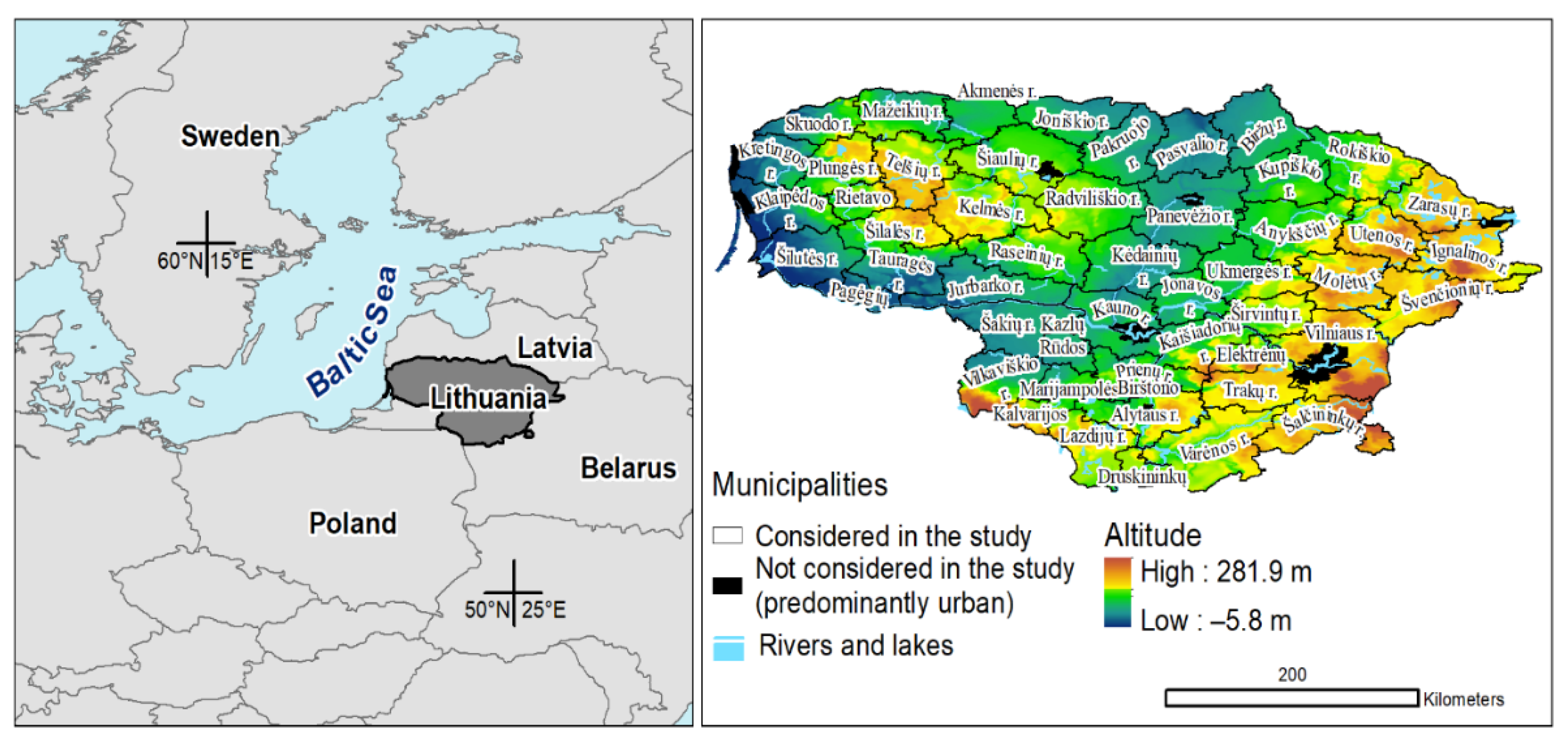
2.1. Study Area
2.2. Input Data
- CORINE databases were acquired from Copernicus Land Monitoring Services (https://land.copernicus.eu/pan-european/corine-land-cover, accessed on 21 December 2021). Here, we used CORINE Land Cover data referring to 1995, 2000, 2006, 2012, and 2018. Hereafter, this data source is referred to as COPERNICUS.
- The borders of municipalities (USE_3 level) available from EuroBoundaryMap (v3.0), which is a European reference database of administrative units and boundaries established within the framework of EuroGeographics (Available online: https://eurogeographics.org/maps-for-europe/ebm/, accessed on 21 December 2021). Hereafter, this data source is referred to as EuroBoundaryMap.
- Soil spatial dataset at a scale of 1:10,000 (Dirv_DR10LT), with the soil productivity grade for each soil polygon. The average soil productivity grade was estimated for agricultural lands in each municipality.
- Land reclamation and wetness dataset at a scale of 1:10,000 (Mel_DR10LT), which was used to estimate the proportion of drained lands for each municipality.
- Dataset of special land-use conditions at a scale of 1:10,000 (SŽNS_DR10LT), which was used to estimate the proportion of lands under specific use restrictions.
- Dataset of abandoned agricultural land (AŽ_DRLT), which was used to characterise the land use intensity in municipalities, estimating the proportion of abandoned land.
- Land parcel block database referring to 2004, 2008, and 2014 (KŽS), containing the borders of agricultural, built-up, miscellaneous (mostly forest), water, and road infrastructure blocks and used to estimate the proportion of specific land use in each municipality.
- River network data from Copernicus Land Monitoring Services (https://land.copernicus.eu/imagery-in-situ/eu-hydro/eu-hydro-river-network-database, accessed on 21 December 2021). The features available from this dataset were intersected with the borders of municipalities to estimate the length of streams per area unit in each municipality.
- Data on the number of residents (JRC-GEOSTAT 2018 dataset) were acquired from the Geographic Information System of the Commission (GISCO) (https://ec.europa.eu/eurostat/web/gisco/geodata/reference-data/population-distribution-demography/geostat, accessed on 21 December 2021). The JRC-GEOSTAT 2018 is a regular grid map of 1 × 1 km cells reporting the number of residents for the year 2018 in Europe. This grid was intersected with the borders of municipalities to obtain the number of residents in municipalities for the year 2018. Additionally, data from Population and Housing Census by Statistics Lithuania (https://osp.stat.gov.lt/gis-duomenys, accessed on 21 December 2021) were used to estimate the population density in each municipality, referring to three dates (1989, 2011, and 2018).
- Data on the transportation network were acquired from the OpenStreetMap project database (https://download.geofabrik.de/, accessed on 21 December 2021). For this study, we calculated the length of linear features per area unit in each municipality for the following road types: motorway/freeway, important roads (typically divided), primary roads (typically national), and secondary roads (typically regional).
- A raster digital terrain model (DTM) from the online service EuroGeographics Open Maps for Europe (https://www.mapsforeurope.org/datasets/euro-dem, accessed on 21 December 2021). In addition to mean, minimum, range, and standard deviation values based on the altitudes, we calculated the same characteristics for the slope and topographic wetness index [24], which were assumed to strongly correlate with soil moisture and provide indirect information on land cover and agricultural potential. Hereafter, this source of data is referred to as MapsForEurope.
- Data on various aspects characterising the agriculture in municipalities, including the intensity of agriculture, were available from the Lithuanian Department of Statistics (Statistics Lithuania).
2.3. Mapping and Evaluating the Land Cover Naturalness
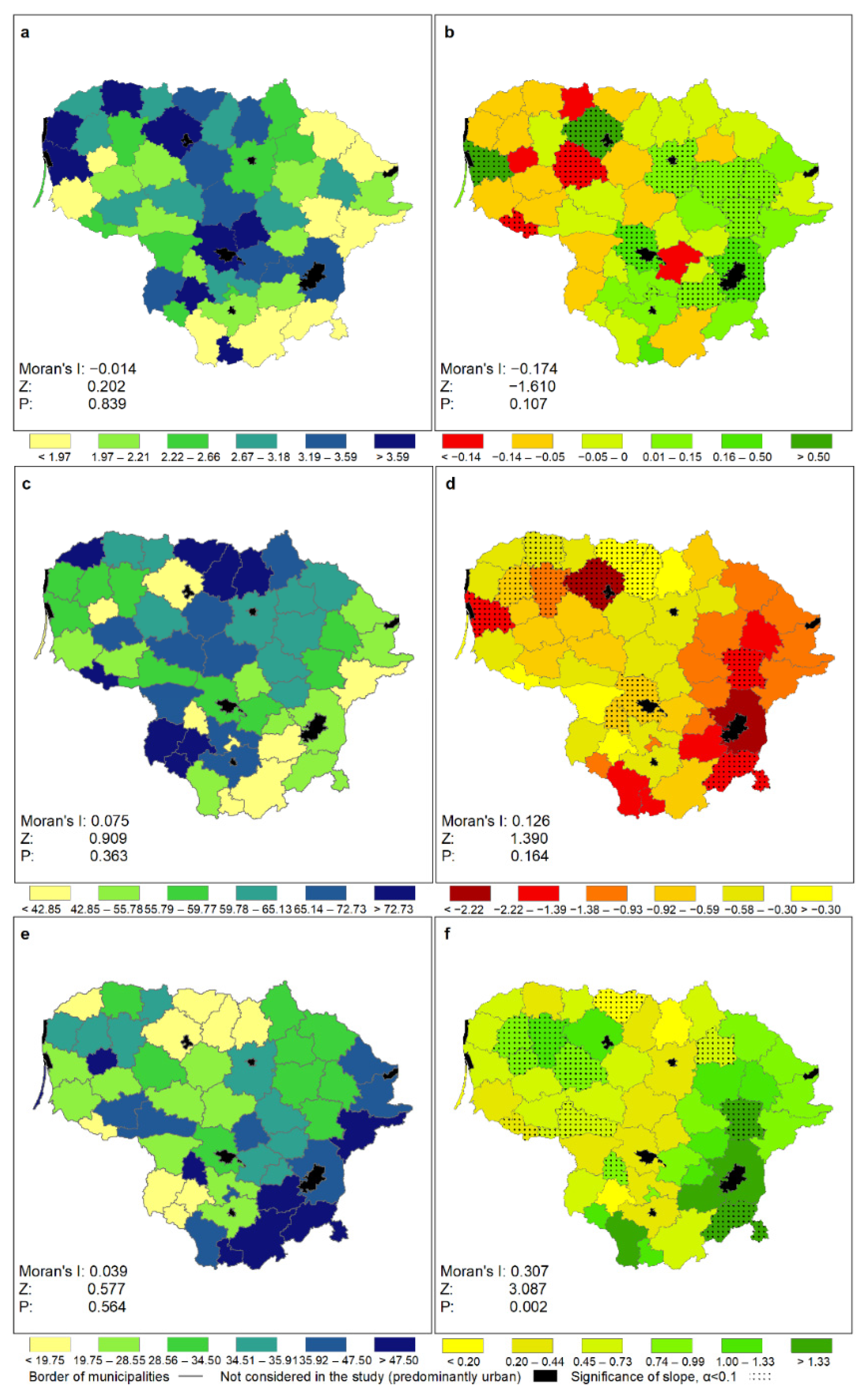
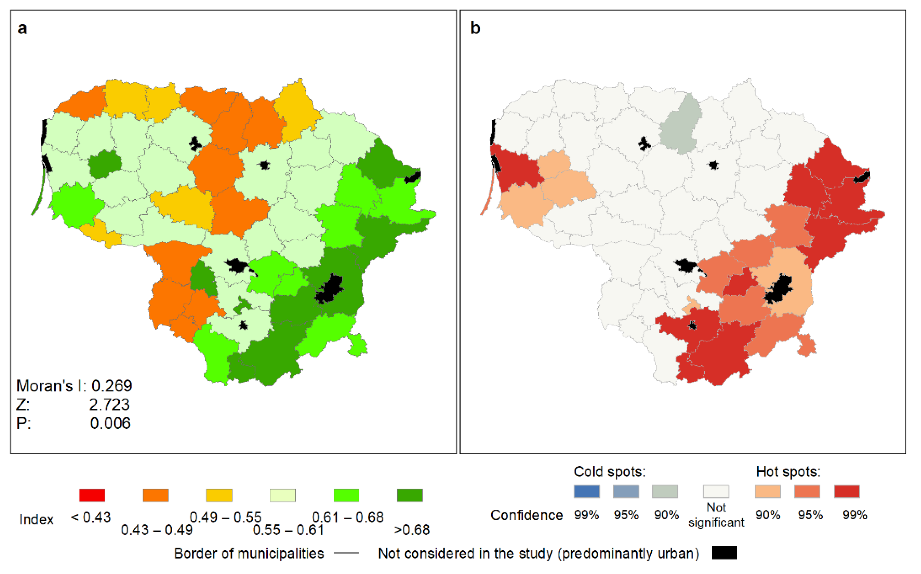
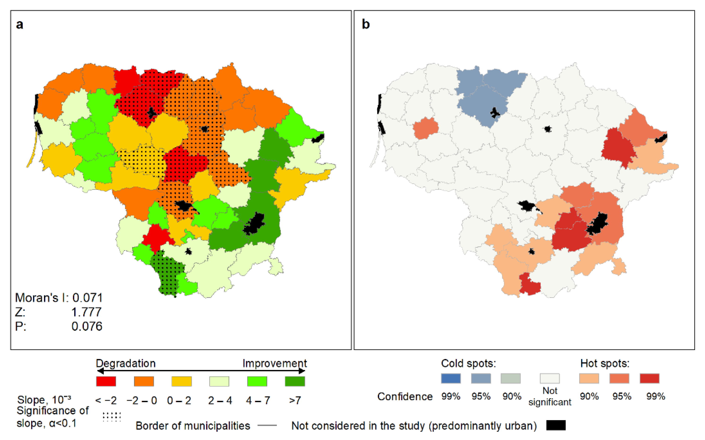
3. Results
4. Discussion
5. Conclusions
Author Contributions
Funding
Institutional Review Board Statement
Informed Consent Statement
Data Availability Statement
Conflicts of Interest
Appendix A

| Class Code | Class Name | Index Value |
|---|---|---|
| 1.1.1 | Continuous urban fabric | 0 |
| 1.1.2 | Discontinuous urban fabric | 0.10 |
| 1.2.1 | Industrial or commercial units | 0 |
| 1.2.2 | Road and rail networks and associated land | 0.10 |
| 1.2.3 | Port areas | 0 |
| 1.2.4 | Airports | 0.10 |
| 1.3.1 | Mineral extraction sites | 0.20 |
| 1.3.2 | Dump sites | 0.10 |
| 1.3.3 | Construction sites | 0.10 |
| 1.4.1 | Green urban areas | 0.50 |
| 1.4.2 | Sport and leisure facilities | 0.30 |
| 2.1.1 | Non-irrigated arable land | 0.30 |
| 2.2.2 | Fruit trees and berry plantations | 0.60 |
| 2.3.1 | Pastures | 0.50 |
| 2.4.1 | Annual crops associated with permanent crops | - |
| 2.4.2 | Complex cultivation patterns | 0.50 |
| 2.4.3 | Land principally occupied by agriculture, with significant areas of natural vegetation | 0.60 |
| 3.1.1 | Broad-leaved forest | 1.00 |
| 3.1.2 | Coniferous forest | 0.90 |
| 3.1.3 | Mixed forest | 1.00 |
| 3.2.1 | Natural grassland | 0.50 |
| 3.2.2 | Moors and heathland | 0.70 |
| 3.2.4 | Transitional woodland/shrub | 0.80 |
| 3.3.1 | Beaches, dunes, sands | 0.70 |
| 3.3.3 | Sparsely vegetated areas | 0.70 |
| 3.3.4 | Burnt areas | 0.50 |
| 4.1.1 | Inland marshes | 1.00 |
| 4.1.2 | Peatbogs | 0.20 |
| 5.1.1 | Water courses | 0.90 |
| 5.1.2 | Water bodies | 0.90 |
| 5.2.1 | Coastal lagoons | 0.90 |
| 5.2.2 | Estuaries | - |
| 5.2.3 | Sea and ocean | 1.00 |
Appendix B
| Alias | Description of the Variable | Source Dataset | Pearson’s Correlation Coefficient * |
|---|---|---|---|
| Characteristics of agriculture | |||
| Cattle number 2009 | Total number of cattle per area unit in the municipality in 2009 | Statistics Lithuania | −0.289 |
| Cattle number 2014 | Total number of cattle per area unit in the municipality in 2014 | Statistics Lithuania | −0.191 |
| Farm number 2009 | Number of farms per area unit, according to the Register of Farmers in 2009 | Statistics Lithuania | 0.228 |
| Farm number 2014 | Number of farms per area unit, according to the Register of Farmers in 2014 | Statistics Lithuania | 0.282 |
| Grassland agric. prop. 2009 | Proportion of the area of perennial grassland from the total agricultural land area in 2009, % | Statistics Lithuania | 0.693 |
| Grassland agric. prop. 2014 | Proportion of the area of perennial grassland from the total agricultural land area in 2009, % | Statistics Lithuania | 0.656 |
| Grassland per cattle unit 2009 | Area of the perennial grassland per one cattle unit in 2009 | Statistics Lithuania | 0.525 |
| Grassland per cattle unit 2014 | Area of the perennial grassland per one cattle unit in 2014 | Statistics Lithuania | 0.530 |
| Grassland total prop. 2009 | Area proportion of the perennial grassland in 2009 | Statistics Lithuania | 0.153 |
| Grassland total prop. 2014 | Area proportion of the perennial grassland in 2014 | Statistics Lithuania | 0.223 |
| Private agric. land prop. 2004 | Area proportion of agricultural land in private lands in 2004 | Statistics Lithuania | −0.523 |
| Private agric. land prop. 2009 | Area proportion of agricultural land in private lands in 2009 | Statistics Lithuania | −0.506 |
| Private agric. land prop. 2014 | Area proportion of agricultural land in private lands in 2014 | Statistics Lithuania | −0.538 |
| Private land per farmer 2009 | Area of private land per one farmer in 2009 | Statistics Lithuania | −0.281 |
| Private land per farmer 2014 | Area of private land per one farmer in 2014 | Statistics Lithuania | −0.305 |
| Private prop. 2009 | Proportion of private land area in 2009 | Statistics Lithuania | −0.262 |
| Private prop. 2014 | Proportion of private land area in 2014 | Statistics Lithuania | −0.300 |
| Conditions for land use | |||
| Drained area prop. | Proportion of drained areas | Mel_DR10LT | −0.773 |
| Soil productivity | Average soil productivity score for agricultural land | Dirv_DR10LT | −0.757 |
| Land covers | |||
| CORINE artificial 1995 | Area proportion of artificial surfaces in 1995 | COPERNICUS | −0.282 |
| CORINE artificial 2000 | Area proportion of artificial surfaces in 2000 | COPERNICUS | −0.278 |
| CORINE artificial 2006 | Area proportion of artificial surfaces in 2006 | COPERNICUS | −0.274 |
| CORINE artificial 2012 | Area proportion of artificial surfaces in 2012 | COPERNICUS | −0.266 |
| CORINE artificial 2018 | Area proportion of artificial surfaces in 2018 | COPERNICUS | −0.265 |
| CORINE agricultural 1995 | Area proportion of agricultural areas in 1995 | COPERNICUS | −0.265 |
| CORINE agricultural 2000 | Area proportion of agricultural areas in 2000 | COPERNICUS | −0.258 |
| CORINE agricultural 2006 | Area proportion of agricultural areas in 2006 | COPERNICUS | −0.259 |
| CORINE agricultural 2012 | Area proportion of agricultural areas in 2012 | COPERNICUS | −0.313 |
| CORINE agricultural 2018 | Area proportion of agricultural areas in 2018 | COPERNICUS | −0.312 |
| CORINE forest1995 | Area proportion of forest and seminatural areas in 1995 | COPERNICUS | 0.383 |
| CORINE forest2000 | Area proportion of forest and seminatural areas in 2000 | COPERNICUS | 0.380 |
| CORINE forest2006 | Area proportion of forest and seminatural areas in 2006 | COPERNICUS | 0.380 |
| CORINE forest2012 | Area proportion of forest and seminatural areas in 2012 | COPERNICUS | 0.443 |
| CORINE forest2018 | Area proportion of forest and seminatural areas in 2018 | COPERNICUS | 0.443 |
| CORINE wetland 1995 | Area proportion of wetlands in 1995 | COPERNICUS | −0.020 |
| CORINE wetland 2000 | Area proportion of wetlands in 2000 | COPERNICUS | −0.003 |
| CORINE wetland 2006 | Area proportion of wetlands in 2006 | COPERNICUS | −0.002 |
| CORINE wetland 2012 | Area proportion of wetlands in 2012 | COPERNICUS | −0.065 |
| CORINE wetland 2018 | Area proportion of wetlands in 2018 | COPERNICUS | −0.063 |
| CORINE water 1995 | Area proportion of water bodies in 1995 | COPERNICUS | 0.167 |
| CORINE water 2000 | Area proportion of water bodies in 2000 | COPERNICUS | 0.162 |
| CORINE water 2006 | Area proportion of water bodies in 2006 | COPERNICUS | 0.162 |
| CORINE water 2012 | Area proportion of water bodies in 2012 | COPERNICUS | 0.162 |
| CORINE water 2018 | Area proportion of water bodies in 2018 | COPERNICUS | 0.162 |
| Land use intensity | |||
| Abandoned prop. | Area proportion of abandoned agricultural land | AŽ_DRLT | 0.600 |
| Agricultural land 2009 | Area proportion of declared land used for agriculture in 2009 | Statistics Lithuania | −0.674 |
| Agricultural land 2014 | Area proportion of declared land used for agriculture in 2014 | Statistics Lithuania | −0.669 |
| Intensive use prop. agric. 2009 | Area proportion of land under intensive use in 2009 | Statistics Lithuania | −0.748 |
| Intensive use prop. agric. 2014 | Proportion of land area under intensive use from total agricultural land in 2009 | Statistics Lithuania | −0.701 |
| Intensive use prop. 2014 | Area proportion of land under intensive use in 2014 | Statistics Lithuania | −0.767 |
| Intensive use prop. 2014 | Proportion of land area under intensive use from total agricultural land in 2014 | Statistics Lithuania | −0.692 |
| Land use restrictions | |||
| Protection zones cult. heritage | Area proportion of cultural heritage protection zones | SŽNS_DR10LT | 0.420 |
| Protection zones electricity | Area proportion of protection zones around electricity lines | SŽNS_DR10LT | −0.021 |
| Protection zones gas | Area proportion of protection zones around gas pipelines | SŽNS_DR10LT | −0.005 |
| Protection zones graveyards | Area proportion of graveyards and protection zones around them | SŽNS_DR10LT | 0.060 |
| Protection zones oil | Area proportion of protection zones around oil pipelines | SŽNS_DR10LT | −0.292 |
| Protection zones protect. areas | Area proportion of protected areas | SŽNS_DR10LT | 0.211 |
| Protection zones railroads | Area proportion of protection zones around railroads | SŽNS_DR10LT | −0.243 |
| Protection zones roads | Area of protection zones around roads | SŽNS_DR10LT | 0.578 |
| Protection zones water | Area proportion of protection zones around water bodies | SŽNS_DR10LT | 0.057 |
| Land uses | |||
| Proportion agricultural 2004 | Area proportion of agricultural blocks in the municipality in 2004 | KŽS | −0.487 |
| Proportion agricultural 2008 | Area proportion of agricultural blocks in the municipality in 2008 | KŽS | −0.488 |
| Proportion agricultural 2014 | Area proportion of agricultural blocks in the municipality in 2014 | KŽS | −0.558 |
| Proportion built-up 2004 | Area proportion of built-up blocks in the municipality in 2004 | KŽS | −0.054 |
| Proportion built-up 2008 | Area proportion of built-up blocks in the municipality in 2008 | KŽS | −0.033 |
| Proportion built-up 2014 | Area proportion of built-up blocks in the municipality in 2014 | KŽS | 0.021 |
| Proportion miscellaneous 2004 | Area proportion of miscellaneous blocks in the municipality in 2004 | KŽS | 0.419 |
| Proportion miscellaneous 2008 | Area proportion of miscellaneous blocks in the municipality in 2008 | KŽS | 0.422 |
| Proportion miscellaneous 2014 | Area proportion of miscellaneous blocks in the municipality in 2014 | KŽS | 0.450 |
| Population | |||
| Pop. count 80th perc. | 80th percentile of the population count | GISCO | −0.327 |
| Pop. count 90th perc. | 90th percentile of the population count | GISCO | −0.305 |
| Pop. density 1989 | Population density in 2011, number of inhabitants/km2 | Statistics Lithuania | −0.141 |
| Pop. density 2011 | Population density in 2018, number of inhabitants/km2 | Statistics Lithuania | −0.017 |
| Pop. density 2018 | Population density in 1989, number of inhabitants/km2 | Statistics Lithuania | −0.427 |
| Terrain | |||
| Max top. wetness index | Maximum value of the topographic wetness index | MapsForEurope | −0.028 |
| Mean altitude | Average altitude within the borders of the municipality | MapsForEurope | 0.591 |
| Mean slope | Average terrain slope within the borders of the municipality | MapsForEurope | 0.591 |
| Mean top. wetness index | Average value of the topographic wetness index | MapsForEurope | −0.689 |
| Min altitude | Minimum altitude value within the borders of the municipality | MapsForEurope | −0.013 |
| Min top. wetness index | Minimum value of the topographic wetness index | MapsForEurope | −0.331 |
| Range altitude | Range of altitude values within the borders of the municipality | MapsForEurope | 0.235 |
| St. dev. altitude | Standard deviation of altitude values within the borders of the municipality | MapsForEurope | 0.427 |
| St. dev. slope | Standard deviation of relief slope values within the borders of the municipality. | MapsForEurope | 0.427 |
| St. dev. top. wetness index | Standard deviation value of the topographic wetness index | MapsForEurope | 0.374 |
| Sum top. wetness index | Sum of the topographic wetness index values | MapsForEurope | −0.211 |
| Topographic elements | |||
| Proportion roads 2004 | Area proportion of roadblocks in the municipality in 2004 | KŽS | 0.116 |
| Proportion roads 2008 | Area proportion of roadblocks in the municipality in 2008 | KŽS | 0.133 |
| Proportion roads 2014 | Area proportion of roadblocks in the municipality in 2014 | KŽS | 0.326 |
| Proportion streams 2004 | Length of streams per area unit in the municipality in 2004 | KŽS | −0.557 |
| Proportion streams 2008 | Length of streams per area unit in the municipality in 2008 | KŽS | −0.582 |
| Proportion streams 2014 | Length of streams per area unit in the municipality in 2014 | KŽS | −0.584 |
| Proportion water bodies 2004 | Area proportion of blocks around the water bodies in the municipality in 2004 | KŽS | 0.376 |
| Proportion water bodies 2008 | Area proportion of blocks around the water bodies in the municipality in 2008 | KŽS | 0.380 |
| Proportion water bodies 2014 | Area proportion of blocks around the water bodies in the municipality in 2014 | KŽS | 0.314 |
| Roads prop. | Length of roads per area unit in the municipality | OpenStreetMap | 0.149 |
| Streams prop. | Length of streams per area unit in the municipality | COPERNICUS | −0.407 |
References
- Houghton, R.A.; Hackler, J.L.; Lawrence, K.T. The U.S. carbon budget: Contributions from land-use change. Science 1999, 285, 575–578. [Google Scholar] [CrossRef] [PubMed]
- DeFries, R.S.; Field, C.B.; Fung, I.; Justice, C.O.; Los, S.; Matson, P.A.; Matthews, E.; Mooney, H.A.; Potter, C.S.; Prentice, P.J.; et al. Mapping the land surface for global atmosphere-biosphere models: Toward continuous distributions of vegetation’s functional properties. J. Geophys. Res. 1999, 100, 20867–20882. [Google Scholar] [CrossRef]
- Sala, O.E.; Chapin, F.S.; Armesto, J.J.; Berlow, E.; Bloomfield, J.; Dirzo, R.; Huber-Sanwald, E.; Huenneke, L.F.; Jackson, R.B.; Kinzig, A.; et al. Biodiversity: Global biodiversity scenarios for the year 2100. Science 2000, 287, 1770–1774. [Google Scholar] [CrossRef] [PubMed]
- Reid, R.S.; Kruska, R.L.; Muthui, N.; Taye, A.; Wotton, S.; Wilson, C.J.; Mulatu, W. Landuse and land-cover dynamics in response to changes in climatic, biological and socio-political forces: The case of southwestern Ethiopia. Landsc. Ecol. 2000, 15, 339–355. [Google Scholar] [CrossRef]
- Wickham, J.D.; O’Neill, R.V.; Jones, K.B. A geography of ecosystem vulnerability. Landsc. Ecol. 2000, 15, 495–504. [Google Scholar] [CrossRef]
- Costanza, R.; Arge, R.; de Groot, R.; Farber, S.; Grasso, M.; Hannon, B.; Limburg, K.; Naeem, S.; Oneill, R.V.; Paruelo, J.; et al. The value of the world’s ecosystem services and natural capital. Nature 1997, 387, 253–260. [Google Scholar] [CrossRef]
- Metzger, M.J.; Rounsevell, M.D.A.; Acosta-Michlik, L.; Leemans, R.; Schröer, D. The vulnerability of ecosystem services to land use change. Agric. Ecosyst. Environ. 2006, 114, 69–85. [Google Scholar] [CrossRef]
- Costanza, R.; de Groot, R.; Sutton, P.C.; van der Ploeg, S.; Anderson, S.; Kubiszewski, I.; Farber, S.; Turner, R.K. Changes in the global value of ecosystem services. Glob. Environ. Chang. 2014, 26, 152–158. [Google Scholar] [CrossRef]
- Brundtland, G. Our Common Future: The World Commission on Environment and Development; Oxford University Press: Oxford, UK, 1987; p. 416. [Google Scholar]
- Renetzeder, C.; Schindler, S.; Peterseil, J.; Prinz, M.A.; Mücher, S.; Wrbka, T. Can we measure ecological sustainability? Landscape pattern as an indicator for naturalness and land use intensity at regional, national and European level. Ecol. Indicators. 2010, 10, 39–48. [Google Scholar] [CrossRef]
- Sauer, C.O. The Morphology of Landscape; University California Press: Berkeley, CA, USA, 1925; Volume 2, p. 37. Available online: https://archive.org/stream/universityofc02univ/universityofc02univ_djvu.txt (accessed on 9 November 2021).
- Wrbka, T.; Erb, K.H.; Schulz, N.B.; Peterseil, J.; Hahn, C.H.; Haberl, H. Linking pattern and process in cultural landscapes. An empirical study based on spatially explicit indicators. Land Use Policy 2004, 21, 289–306. [Google Scholar] [CrossRef]
- Lamb, R.J.; Purcell, T. Perception of naturalness in landscape and its relationship to vegetation structure. Landsc. Urban Plan. 1990, 9, 333–352. [Google Scholar] [CrossRef]
- Tuluhan Yılmaz, K.; Alphan, H.; Gülçin, D. Assessing Degree of Landscape Naturalness in a Mediterranean Coastal Environment Threatened by Human Activities. J. Urban Plan. Dev. 2019, 145. [Google Scholar] [CrossRef]
- Vinclovaitė, G.; Veteikis, D. Kraštovaizdžio poliarizacijos metodologinės problemos [The problems of landscape polarization methodology]. Geogr. T. 2001, 47, 38–45. [Google Scholar]
- Skorupskas, R. Kraštovaizdžio Struktūros Geoekologinio Optimalumo Metodologija (Lietuvos Teritorijos Pavyzdžiu) [Methodology of Geoecological Optimization of Landscape Structure (Lithuania as a case)]. Ph.D. Thesis, Vilniaus Universitetas, Vilnius, Lithuania, 2006. [Google Scholar]
- Vaitkuvienė, D.; Dagys, M. Lietuvos CORINE Žemės Danga 2006. Ataskaita [Lithuanian CORINE Land Cover 2006. Final Report]; Ekologijos Institutas: Vilnius, Lithuania, 2008. [Google Scholar]
- Kairiūkštis, L. Miškų priešistorė ir teritorijos miškingumo kaita [Pre-History of Forests and Change of Forest Area Proportion]. In Lietuvos Miškų Metraštis XX a. [The Cronicle of Lithuanian Forests XX Century]; Kairiukštis, L., Ed.; Department of Forests, Ministry of Environment of the Republic of Lithuania: Vilnius, Lithuania, 2003; pp. 19–23. [Google Scholar]
- Juknelienė, D.; Mozgeris, G. The spatial pattern of forest cover changes in Lithuania during the second half of the twentieth century. Žemės Ūkio Moksl. 2015, 22, 209–215. [Google Scholar] [CrossRef] [Green Version]
- Juknelienė, D.; Valčiukienė, J.; Atkocevičienė, V. Assessment of regulation of legal relations of territorial planning: A case study in Lithuania. Land Use Policy 2017, 67, 65–72. [Google Scholar] [CrossRef]
- Juknelienė, D.; Kazanavičiūtė, V.; Valčiukienė, J.; Atkocevičienė, V.; Mozgeris, G. Spatiotemporal Patterns of Land-Use Changes in Lithuania. Land 2021, 10, 619. [Google Scholar] [CrossRef]
- Plan of the Territory of the Republic of Lithuania. Available online: file:///C:/Users/Daiva/AppData/Local/Temp/II%20dalis.%202.1.%20Kra%C5%A1tovaizd%C5%BEio%20naudojimas%20ir%20apsauga.pdf (accessed on 9 December 2021).
- Veteikis, D.; Jukna, L.; Jankauskaitė, M. Kraštovaizdžio Struktūros Pokyčių Probleminiuose Arealuose Vertinimas Vietiniu Lygmeniu. 2015 [Assessment of Landscape Structure in problematic Areas at Local Level]. Available online: https://old.gamta.lt/files/Ataskaita%202016-01-13.pdf (accessed on 9 December 2021).
- Moore, I.D.; Grayson, R.B.; Ladson, A.R. Digital terrain modelling: A review of hydrological, geomorphological, and biological applications. Hydrol. Processes 1991, 5, 3–30. [Google Scholar] [CrossRef]
- Salmi, T.; Anu Määttä, A.; Anttila, P.; Ruoho-Airola, T.; Amnell, T. Detecting Trends of Annual Values of Atmospheric Pollutants by the Mann-Kendall Test and Sen’s Slope Estimates—The Excel Template Application MAKESENS; Finnish Meteorological Institute: Helsinki, Finland, 2002; p. 35. Available online: https://www.researchgate.net/publication/259356944 (accessed on 9 December 2021).
- Veteikis, D.; Jankauskaitė, M. Urbanizuotos aplinkos monitoringo sistemos elementai ir jų skyrimo problema [Elements of urban environment monitoring system and problem of their distinguishing]. Geogr. Metraštis 2004, 37, 95–105. [Google Scholar]
- Antrop, M. Rural-Urban Conflicts and Opportunities. The New Dimensions of the European Landscape; Springer: Dordrecht, The Netherlands, 2004; pp. 83–91. [Google Scholar]
- Antrop, M. From Holistic Landscape Synthesis to Transdisciplinary Landscape Management. In From Landscape Research to Landscape Planning—Aspects of Integration, Education and Application; Tress, B., Tres, G., Fry, G., Opdam, P., Eds.; UGent Publication: Gand, Belgique, 2006; pp. 27–50. [Google Scholar]
- Veteikis, D. Polinė ląstelinė kultūrinio kraštovaizdžio struktūra. 1. Teoriniai aspektai. [Polarized cellular structure of cultural landscape: 1. Theoretic aspects]. Ann. Geogr. 2007, 40, 3–13. [Google Scholar]
- Bukantis, A.; Gedžiūnas, P.; Giedraitienė, J.; Ignatavičius, G.; Jonynas, J.; Kavaliauskas, P.; lazauskienė, J.; Reipšleger, R.; Sakalauskienė, G.; Sinkevičius, S.; et al. Lietuvos Gamtinė Aplinka, Būklė, Procesai ir Raida [Lithuanian Natural Environment, Condition, Processes and Development]; Petro Ofsetas: Vilnius, Lithuania, 2008. [Google Scholar]
- Tzanopoulos, J.; Vogiatzakis, I.N. Processes and patterns of landscape change on a small Aegean island: The case of Sifnos, Greece. Landsc. Urban Plan. 2011, 99, 58–64. [Google Scholar] [CrossRef]
- Li, J.; Pu, R.; Gong, H.; Luo, X.; Ye, M.; Feng, B. Evolution Characteristics of Landscape Ecological Risk Patterns in Coastal Zones in Zhejiang Province, China. Sustainability 2017, 9, 584. [Google Scholar] [CrossRef] [Green Version]
- Sowinska-Swierkosz, B.; Michalik-Sniezek, M. The Methodology of Landscape Quality (LQ) Indicators Analysis Based on Remote Sensing Data: Polish National Parks Case Study. Sustainability 2020, 12, 2810. [Google Scholar] [CrossRef] [Green Version]
- Wang, H.; Liu, X.; Zhao, C.; Chang, Y.; Liu, Y.; Zang, F. Spatial-temporal pattern analysis of landscape ecological risk assessment based on land use/land cover change in Baishuijiang National nature reserve in Gansu Province, China. Ecol. Indic. 2021, 124, 107454. [Google Scholar] [CrossRef]
- National Atlas [Nacionalinis Atlasas]. Available online: https://www.geoportal.lt/geoportal/lietuvos-nacionalinis-atlasas#savedSearchId={9A25FCCB-BCC2-4DDB-A5E5-A2D4F6B3952D}&collapsed=true; (accessed on 12 January 2022).
- Kulbokas, G.; Jurevičienė, V.; Kuliešis, A.; Augustaitis, A.; Petrauskas, E.; Mikalajūnas, M.; Vitas, A.; Mozgeris, G. Fluctuations in gross volume increment estimated by the Lithuanian National Forest Inventory compared with annual variations in single tree increment. Balt. For. 2019, 25, 105–112. [Google Scholar] [CrossRef]
- Kuliešis, A.; Kasperavičius, A.; Kulbokas, G. Lithuania (Book Chapter) National Forest Inventories: Assessment of Wood Availability and Use; Springer: Cham, Switzerland, 2016; pp. 521–547. [Google Scholar]
- Mozgeris, G.; Brukas, V.; Pivoriūnas, N.; Činga, G.; Makrickiene, E.; Byčenkienė, S.; Marozas, V.; Mikalajūnas, M.; Dudoitis, V.; Ulevičius, V.; et al. Spatial pattern of climate change effects on Lithuanian forestry. Forests 2019, 10, 809. [Google Scholar] [CrossRef] [Green Version]
- Maziliauskas, A.; Morkunas, V.; Rimkus, Z.; Šaulys, V. Economic incentives in land reclamation sector in Lithuania. J. Water Land Dev. 2007, 11, 17–30. [Google Scholar] [CrossRef]
- Mardosa, J. Lithuania’s Rural Settlements Structural Transformations in Soviet and Post-Soviet Period. In Liquid Structures and Cultures; Kozlova, O., Kołodziej, A., Eds.; Uniwersytet Szczeciński: Szczecin, Poland, 2017; pp. 161–176. [Google Scholar]
- Šaulys, V.; Barvidienė, O. Substantiation of the expediency of drainage systems renovation in Lithuania. In Proceedings of the 9th International Conference Environmental Engineering, Vilnius, Lithuania, 22–23 May 2014. [Google Scholar] [CrossRef]
- Order No. 3D-130/D1-144, 2004. Available online: https://e-seimas.lrs.lt/portal/legalAct/lt/TAD/TAIS.230808/asr (accessed on 12 January 2022).
- Dumbrauskas, A. Melioracijos Griovių Būklės Vertinimas Taikant Nuotolinius Tyrimo Metodus: Galutinė Ataskaita [Assessment of Condition of Drainage Systems Using Remote Sensing Methods: Final Report]; Aleksandro Stulginskio Universitetas: Kaunas, Lithuania, 2017; p. 112. Available online: https://zum.lrv.lt/uploads/zum/documents/files/LT_versija/Veiklos_sritys/Mokslas_mokymas_ir_konsultavimas/Moksliniu_tyrimu_ir_taikomosios_veiklos_darbu_galutines_ataskaitos/2017/Melioracijos%20griovi%C5%B3%20b%C5%ABkl%C4%97s%20vertinimas%20taikant%20nuotolinius%20tyrimo%20metodus.pdf (accessed on 25 January 2022).
- Bilsborrow, R.E.; Okoth-Ogendo, H.W.O. Population-Driven Changes in Land Use in Developing Countries. Ambio 1992, 21, 37–45. [Google Scholar]
- Heilig, G.K. Neglected Dimensions of Global Land-Use Change: Reflections and Data. Popul. Dev. Rev. 1994, 20, 831. [Google Scholar] [CrossRef]
- Azadi, H.; Ho, P.; Hasfiati, L. Agricultural land conversion drivers: A comparison between less developed, developing and developed countries. Land Degrad. Dev. 2010, 22, 596–604. [Google Scholar] [CrossRef]
- Chen, R.S.; Ye, C.; Cai, Y.L.; Xing, X.S.; Chen, Q. The impact of rural out-migration on land use transition in China: Past, present and trend. Land Use Policy 2014, 40, 101–110. [Google Scholar] [CrossRef]
- Skog, K.L.; Steinnes, M. How do centrality, population growth and urban sprawl impact farmland conversion in Norway? Land Use Policy 2016, 59, 185–196. [Google Scholar] [CrossRef]
- Haarsma, D.; Qiu, F. Assessing Neighbor and Population Growth Influences on Agricultural Land Conversion. Appl. Spat. Anal. Policy 2017, 10, 21–41. [Google Scholar] [CrossRef]
- Tong, Q.; Qiu, F. Population growth and land development: Investigating the bi-directional interactions. Ecol. Econ. 2020, 169, 106505. [Google Scholar] [CrossRef]
- Ministry of Environment. Lithuanian Statistical Yearbook of Forestry; Ministry of Environment, State Forest Service: Kaunas, Lithuania, 2020; Available online: http://www.amvmt.lt/index.php/leidiniai/misku-ukio-statistika/2020 (accessed on 4 January 2022).
- National Forest Agreement. Available online: https://nacionalinismiskususitarimas.lt (accessed on 4 January 2022).
- Decision No. 569, 2012. Available online: https://e-seimas.lrs.lt/portal/legalAct/lt/TAD/TAIS.425608 (accessed on 12 January 2022).
- Order No. D1-199, 2008. Available online: https://www.e-tar.lt/portal/lt/legalAct/TAR.E0061030F4E1/asr (accessed on 12 January 2022).
- Decision No. 1131, 2011. Available online: https://e-seimas.lrs.lt/portal/legalAct/lt/TAD/TAIS.407618?jfwid=-1n2mj1nis (accessed on 12 January 2022).
- 2014–2020 Rural Development Programme—Lithuania. Available online: https://ec.europa.eu/info/food-farming-fisheries/key-policies/common-agricultural-policy/rural-development/country/lithuania_lt (accessed on 12 January 2022).
- Regulation (EU) 2021/2115 of the European Parliament of the Council, 2021. Available online: https://eur-lex.europa.eu/eli/reg/2021/2115 (accessed on 12 January 2022).
- Order No. D1-703, 2015. Available online: https://e-seimas.lrs.lt/portal/legalAct/lt/TAD/TAIS.425608 (accessed on 12 January 2022).
- The European Green Deal. Available online: https://eur-lex.europa.eu/legalcontent/EN/TXT/?qid=1576150542719&uri=COM%3A2019%3A640%3AFIN (accessed on 18 February 2022).
- A Farm to Fork strategy. Available online: https://eur-lex.europa.eu/legal-content/EN/TXT/?uri=CELEX:52020DC0381 (accessed on 18 February 2022).
- EU Biodiversity Strategy for 2030. Available online: https://eur-lex.europa.eu/legal-content/EN/TXT/?qid=1590574123338&uri=CELEX:52020DC0380 (accessed on 18 February 2022).
- European Commission, Directorate-General for Research and Innovation, A Sustainable Bioeconomy for Europe: Strengthening the Connection Between Economy, Society and the Environment: Updated Bioeconomy Strategy, Publications Office, 2018. Available online: https://data.europa.eu/doi/10.2777/478385 (accessed on 19 February 2022).


| Variable | Ordinary Least Squares Linear Regression | Geographically Weighted Regression | ||||||
|---|---|---|---|---|---|---|---|---|
| Akaike Information Criterion | Adjusted R2 | Jarque–Bera Statistic | Koenker (BP) Statistic | Moran’s I of Residuals | Akaike Information Criterion | Adjusted R2 | Moran’s I of Residuals | |
| Average area proportion during the period since 1995 of: | ||||||||
| Artificial surfaces | −431 | 0.051 | 1.541 | 0.576 | 0.267 | −441 | 0.285 | 0.059 |
| Agricultural areas | −431 | 0.049 | 0.515 | 2.699 | 0.317 | −437 | 0.280 | 0.204 |
| Forest and seminatural areas | −435 | 0.110 | 1.355 | 0.679 | 0.277 | −438 | 0.237 | 0.184 |
| Wetlands | −428 | −0.017 | 1.761 | 0.283 | 0.343 | −437 | 0.304 | 0.140 |
| Water bodies | −429 | 0.007 | 0.937 | 5.599 | 0.319 | −446 | 0.382 | 0.179 |
| Slope of the linear trend in changes during the period since 1995 of: | ||||||||
| Artificial surfaces | −428 | −0.020 | 1.684 | 1.200 | 0.331 | −441 | 0.333 | 0.182 |
| Agricultural areas | −446 | 0.289 | 28.974 | 10.545 | 0.298 | −463 | 0.561 | 0.238 |
| Forest and seminatural areas | −463 | 0.474 | 10.578 | 1.493 | 0.392 | −475 | 0.691 | 0.220 |
| Wetlands | −430 | 0.030 | 1.734 | 0.394 | 0.310 | −437 | 0.245 | 0.147 |
| Water bodies | −428 | −0.018 | 1.573 | 0.000 | 0.336 | −436 | 0.261 | 0.154 |
| Adjusted R2 | Corrected Akaike Information Criterion | Jarque–Bera Statistic | Koenker (BP) Statistic | Variance Inflation Factor | Moran’s I of the Regression Residuals | Model |
|---|---|---|---|---|---|---|
| Three explanatory variables | ||||||
| 0.784 | −494.8 | 0.33 | 0.76 | 1.38 | 0.88 | 0.012869 − 0.000119 × [Drained area prop.] *** − 0.000076 × [Intensive use prop. 2014] *** − 0.001521 × [CORINE wetland 2012] *** |
| 0.781 | −494.2 | 0.33 | 0.63 | 1.29 | 0.91 | 0.006178 − 0.000125 × [Drained area prop.] *** + 0.000073 × [Grassland agric. prop. 2014] *** − 0.001522 × [CORINE wetland 2012] *** |
| 0.754 | −488.2 | 0.48 | 0.13 | 2.04 | 0.94 | −0.011206 + 0.000181 × [Grassland agric. prop. 2009] *** − 0.000258 × [Grassland total prop. 2009] *** − 0.000001 × [Protection zones roads] *** |
| Two explanatory variables | ||||||
| 0.715 | −482.0 | 0.97 | 0.08 | 1.01 | 0.71 | 0.002914 + 0.000124 × [Grassland agric. prop. 2009] *** − 0.000001 × [Proportion streams 2004] *** |
| 0.712 | −481.4 | 0.51 | 0.24 | 1.33 | 0.89 | 0.003456 − 0.000107 × [Drained area prop.] *** + 0.000079 × [Grassland agric. prop. 2009] *** |
| 0.711 | −481.4 | 0.90 | 0.10 | 1.01 | 0.82 | 0.014212 − 0.000124 × [Intensive use prop. agric. 2014] *** − 0.000001 × [Proportion streams 2004] *** |
| One explanatory variable | ||||||
| 0.589 | −464.7 | 0.57 | 0.09 | 1.00 | 0.62 | 0.008781 − 0.000145 × [Drained area prop.] *** |
| 0.580 | −463.5 | 0.52 | 1.00 | 1.00 | 0.28 | 0.006734 − 0.000187 × [Intensive use prop. 2014] *** |
| 0.565 | −461.7 | 0.85 | 0.16 | 1.00 | 0.43 | 0.023713 − 0.000534 × [Soil productivity] *** |
| 0.551 | −460.1 | 0.62 | 0.82 | 1.00 | 0.27 | 0.006237 − 0.000199 × [Intensive use prop. agric. 2009] *** |
Publisher’s Note: MDPI stays neutral with regard to jurisdictional claims in published maps and institutional affiliations. |
© 2022 by the authors. Licensee MDPI, Basel, Switzerland. This article is an open access article distributed under the terms and conditions of the Creative Commons Attribution (CC BY) license (https://creativecommons.org/licenses/by/4.0/).
Share and Cite
Juknelienė, D.; Česonienė, L.; Jonikavičius, D.; Šileikienė, D.; Tiškutė-Memgaudienė, D.; Valčiukienė, J.; Mozgeris, G. Development of Land Cover Naturalness in Lithuania on the Edge of the 21st Century: Trends and Driving Factors. Land 2022, 11, 339. https://doi.org/10.3390/land11030339
Juknelienė D, Česonienė L, Jonikavičius D, Šileikienė D, Tiškutė-Memgaudienė D, Valčiukienė J, Mozgeris G. Development of Land Cover Naturalness in Lithuania on the Edge of the 21st Century: Trends and Driving Factors. Land. 2022; 11(3):339. https://doi.org/10.3390/land11030339
Chicago/Turabian StyleJuknelienė, Daiva, Laima Česonienė, Donatas Jonikavičius, Daiva Šileikienė, Daiva Tiškutė-Memgaudienė, Jolanta Valčiukienė, and Gintautas Mozgeris. 2022. "Development of Land Cover Naturalness in Lithuania on the Edge of the 21st Century: Trends and Driving Factors" Land 11, no. 3: 339. https://doi.org/10.3390/land11030339