Article

A Multi-Scenario Land Expansion Simulation Method from Ecosystem Services Perspective of Coastal Urban Agglomeration: A Case Study of GHM-GBA, China

1
School of Architecture, Tianjin University, Tianjin 300072, China
2
Institute of Urban Space and Urban Design, School of Architecture, Tianjin University, Tianjin 300072, China
*
Author to whom correspondence should be addressed.
Land 2022, 11(11), 1934; https://doi.org/10.3390/land11111934
Submission received: 11 October 2022 / Revised: 24 October 2022 / Accepted: 27 October 2022 / Published: 30 October 2022
(This article belongs to the Special Issue Territory Spatial Planning toward High-Quality Development in China)

Abstract

:
Balancing urban development and ecosystem conservation in the context of natural resource scarcity can provide scientific guidance for land use planning. We integrated research methods, such as ecosystem services (ES) assessment, coastal vulnerability assessment, multi-objective linear planning, and land use change simulation, to develop a new model framework for multi-scenario urban land expansion simulation based on ecosystem services. In relation to the land use scale and constraints, we simulated three types of scenarios in 2035, including a status quo continuity scenario (SCS), economic development scenario (EDS), and ecological protection scenario (EPS), to explore the ideal land use optimization strategies to enhance ES and land use efficiency. The results indicated that the scale of construction land under the three scenarios grew, and arable land and grassland had the largest losses. The continued urban expansion in the Guangdong–Hong Kong–Macao Greater Bay Area has already had a significant negative impact on ecosystem services and could result in a total ESV loss of USD 28.1 billion by 2035 if an economic-first development model is adopted. Based on the hotspots of urban construction land expansion in the ecological–economic priority game, we proposed a classification and optimization strategy for land use, including proactive restoration of damaged ecological spaces with high ESVs (Zhaoqing City and Huizhou City), optimization of green space quality and formation of ecological corridors (Guangzhou City, Shenzhen City, Hong Kong, and Macao), and implementation of natural resource conservation planning and spatial regulation in the urban–rural integration area (Foshan City and Dongguan City). This research framework scientifically allocates the “quality” of ecosystem values and “quantity” of natural resources and provides a reference for regional “bottom-up” territorial spatial planning.

1. Introduction

Climate change exacerbates land degradation processes in the form of floods, heat stress, and sea level rises, causing irreversible impacts on ecosystems [1,2]. Many international environmental organizations, such as the Food and Agriculture Organization of the United Nations (FAO) and International Union of Nature Conservation (IUCN), have proposed the ecosystem approach as a climate change response strategy without negative effects, and countries worldwide should strive to achieve climate change mitigation through self-adaptation of ecosystems [3,4]. However, because of its past long-term rough economic development model, China’s urbanization process has driven rapid expansion of construction land, and urban agglomerations have become highly sensitive areas for intensification of conflicts between humans and nature [
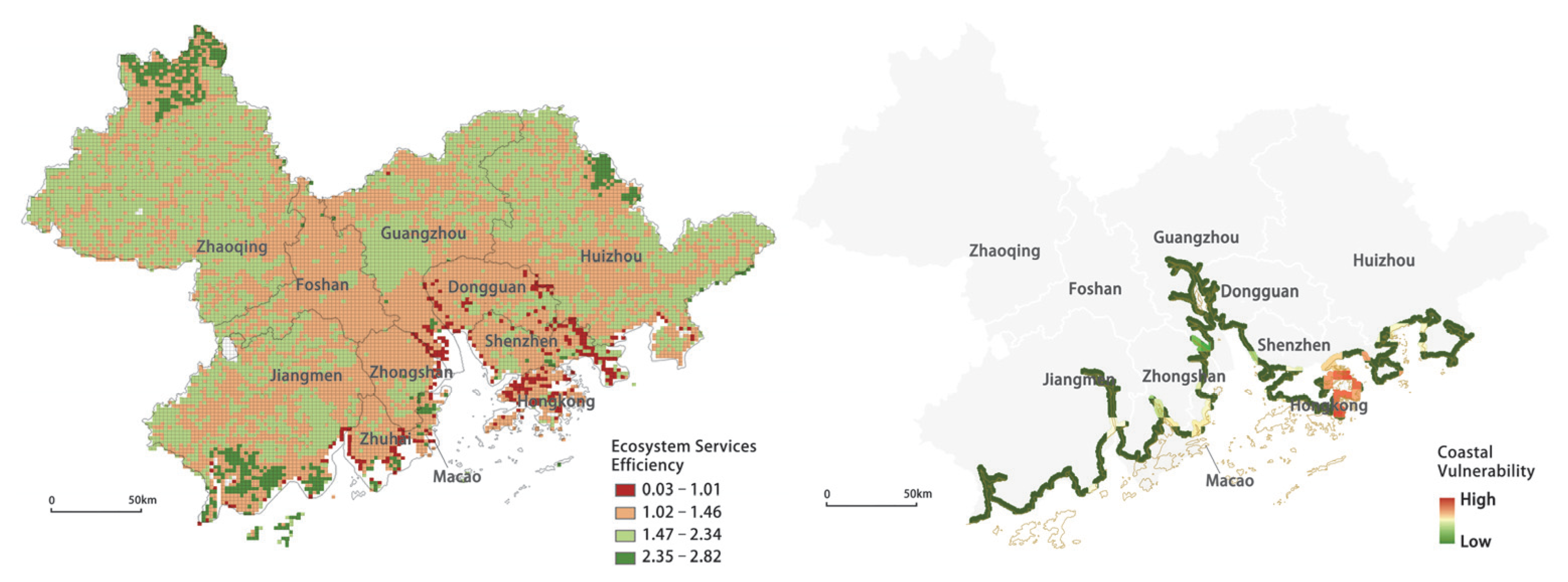
5]. Even in the process of urban cluster selection and cultivation, disregard for resources and ecological environment carrying capacity has led to a long-term spatial mismatch between construction land and ecological land, which has caused a variety of environmental problems. Especially in coastal areas, under the influence of industrial development and port and town expansion, ecological functions, such as the biodiversity and coastal zone nutrient circulation provided by coastal mangroves, are receding, and coastal cities are facing natural disasters and risks, such as sea level rise and storm surges [6]. Transmutation of urban form requires establishment of a new order of ecological civilization. As a new form of transformation and development of today’s cities from traditional single cities to urban communities, the cultivation and development process of urban agglomerations should take into full consideration resource and environmental bearing factors. Promoting the quality and stability of ecosystem services is of great significance to the construction of ecological civilization in urban agglomerations.
Urban spatial expansion is closely related to the rapid urbanization and spatial reconfiguration of urban agglomerations. Since the concept of growth management was proposed in the United States in the 1990s, a look at the 30-year history of urban spatial expansion and management has been accompanied by urban problems, such as urban sprawl, ecological space damage, and dependence on motor vehicles for land development, which have had a series of negative impacts on society, the economy, and ecosystems. In this context, the study of land expansion characteristics has become the focus of scholars at the domestic and international level in recent years, and rich results have been achieved through in-depth research on time sequence, space, and development quality of land expansion [7,8]. With the development of geographic information technology and improvement in statistical models, more scholars have conducted research on the intensity of land expansion and urban development factors. Ma et al. measured the urban expansion index (UEI) and spatial correlation index of 30 cities in five provinces of the Central Plains Urban Agglomeration, and the results showed that the urban agglomeration has experienced a process from “jumping discrete expansion” to “ladder circle expansion” since 2006, and the distribution of construction land in each city is more balanced [9]. Dutta et al. analyzed the spatial and temporal patterns of impervious surface growth in Delhi and its surrounding areas using remote sensing satellite images from 2003 and 2014 and showed a strong negative correlation between urban impervious surface and UEI [10]. Compared with the land expansion mechanism of individual cities, the expansion of construction land under the scale of urban agglomerations is influenced by economic, social, and geographical factors, and some scholars have turned to the flow of information elements and the spatial neighborhood effects of urban agglomerations to study the land expansion in recent years. New features and directions have emerged in the studies of expansion characteristics based solely on land use changes, but the core demand to solve the ecological problems that arise in the process of land expansion has not changed significantly.
Ecosystem services (ES) are the bridge between ecosystems and the urban environment and refer to the benefits that humans derive directly or indirectly from ecosystems. In other words, ES are the natural environmental conditions and utilities that ecosystems provide to sustain human existence [11]. Global ecosystem services have been extensively degraded, leading to irreversible loss of ecosystem service values (ESVs). ESVs estimate the ES and natural capital created using economic laws and are also an intuitive value for quantifying ES. Among all human activities, land use/land cover (LULC) change is the main factor affecting the functional degradation of multiple types of ES [12]. The impact of LULC on ES varies significantly across ecological, social, and economic environments and spatiotemporal scales, especially in mega-urbanized areas. In Delhi during the period 2003–2010, the net reduction increased to USD 40/ha/year in ecosystem services. Urban development activities are largely dependent on consumption of ecosystem services produced [13]. Coastal development and urbanization have led to severe degradation of about 30% of the mangrove forests in the southeastern coastal urban agglomeration of Brazil, and the biodiversity conservation, habitat provision, shoreline protection, and nutrient supply provided by mangroves is deteriorating [14]. In recent years, scholars have achieved a series of productive results in the study of ES and LULC [15]. At the research scale, the relationship between land use and ES in watersheds, coastal wetlands, water-bearing lands, and urbanized areas has been explored [16,17]. In terms of research content, ES is used as a basis for constructing ecological resistance surfaces, ecological safety patterns, and ecological health patterns and for predicting urban land expansion processes. In terms of simulation methods, urban expansion models (CLUE-S, SLEUTH, FLUS, PLUS) based on the principle of cellular automata are mostly used, which are compatible with various types of algorithms and closely integrated with the GIS spatial database and remote sensing data and can predict the scale and scope of urban land expansion under different scenarios [18,19]. Valuation of ecosystem services and their values has become one of the hot research areas in multiple disciplines. Research methods and research tools have been increasingly improved, but further research is needed on how to integrate ecosystem services from an eco-social system perspective into the spatial planning system and constrain the spatial expansion of land through the spatial heterogeneity of ecosystem services.
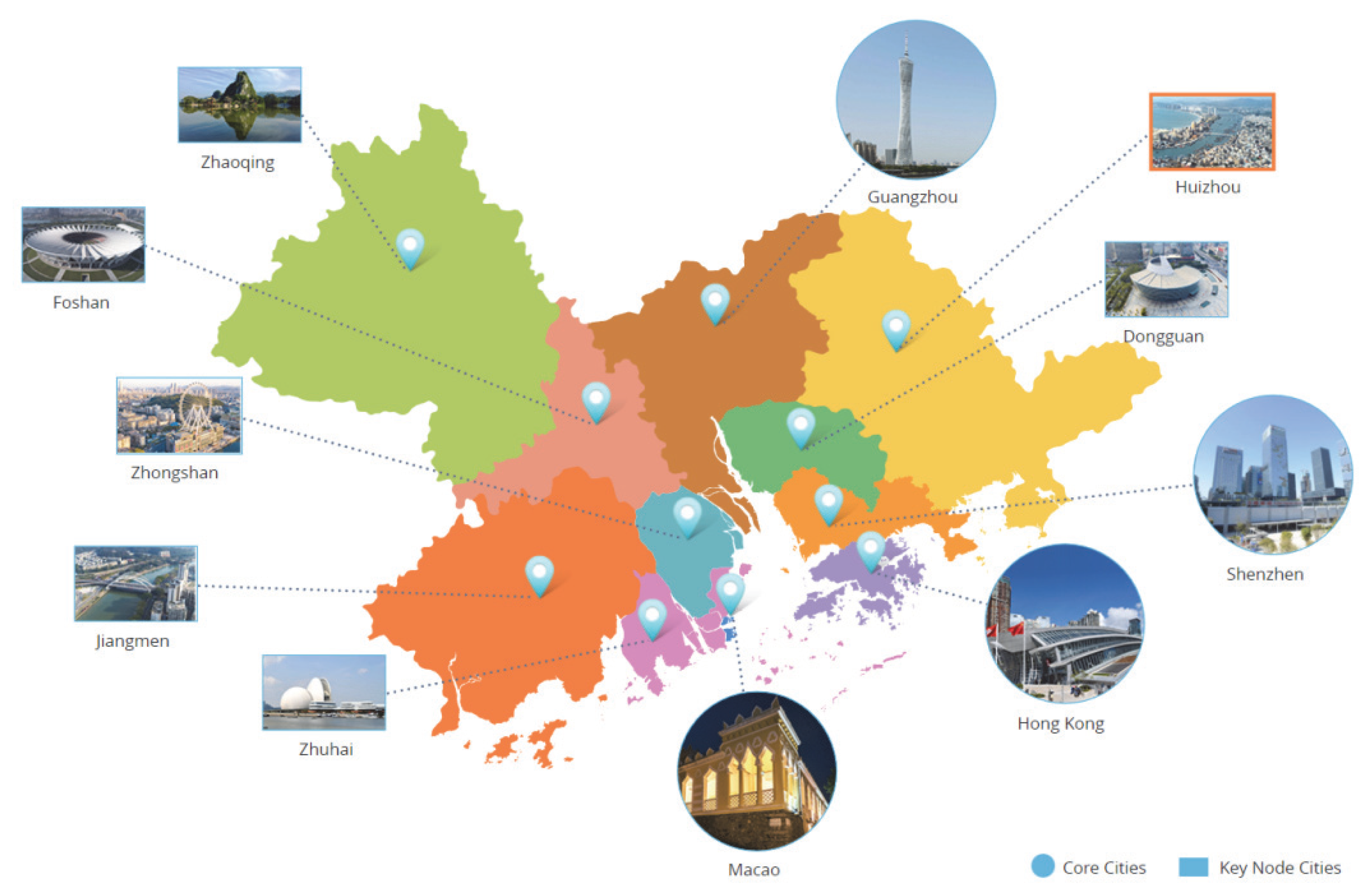
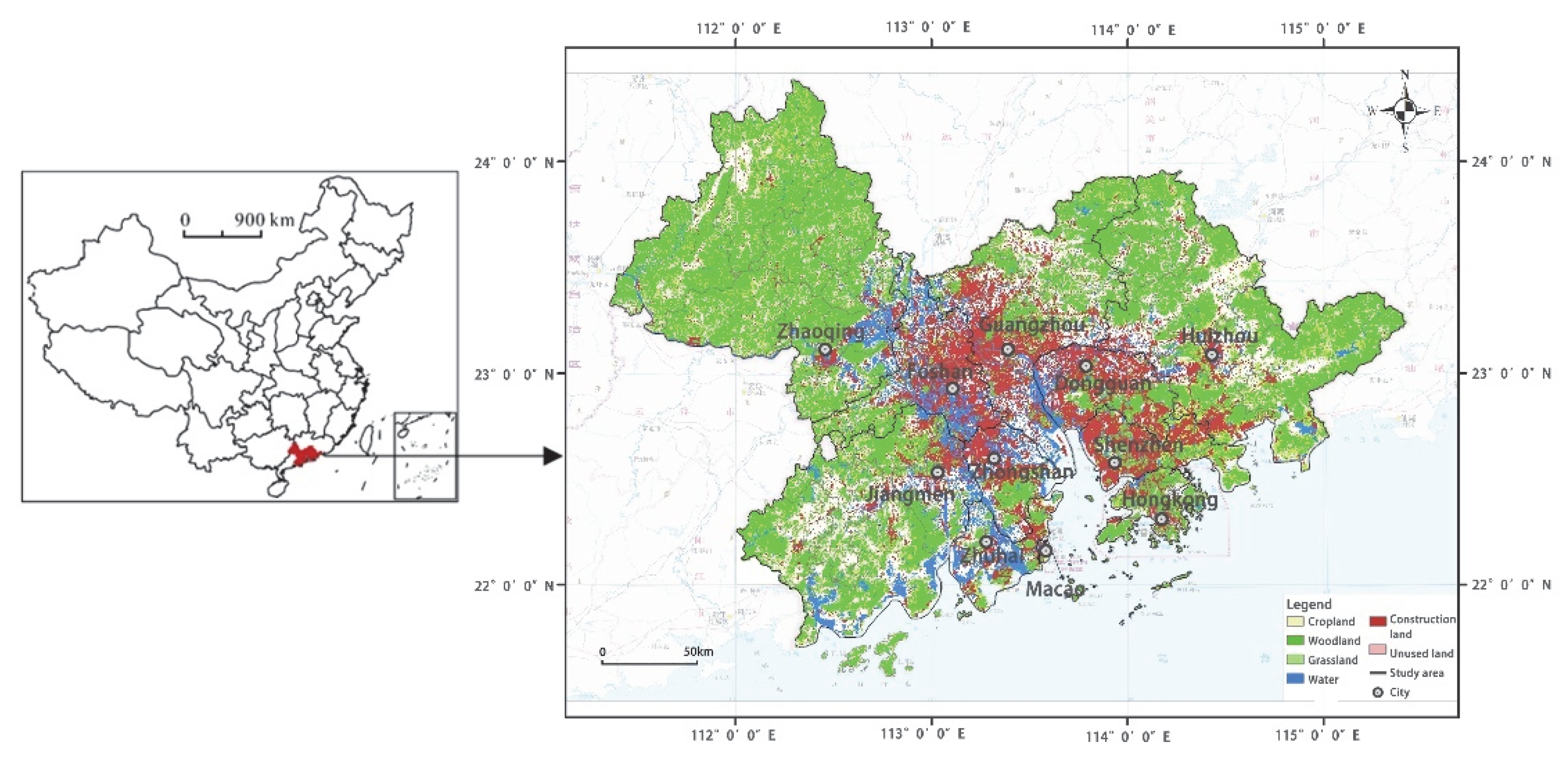
In summary, existing studies have focused on exploring the dynamic correlation patterns between historical land use and ESVs or exploring the spatial growth trends of towns and cities based on historical patterns. However, the impact of ecological space protection needs, policy regulation, and constraints on urban land expansion is less addressed, resulting in the ecological response always taking a passive defense position after major events in the process of urban development. Research scales are also mostly based on municipal and provincial perspectives, with fewer studies from the perspective of typical urban agglomerations. Therefore, this paper proposes a multi-scenario urban land expansion simulation model based on ES, builds a simulation model of urban land expansion coupled with the spatial pattern of ecosystem services based on the concept of ecosystem services, and quantitatively analyzes the spatiotemporal feedback between urban land expansion and ecosystem services in urban agglomerations. In this paper, the Guangdong–Hong Kong–Macao Greater Bay Area (GHM-GBA) is used as a case study. The San Francisco Bay Area and New York Bay Area in the US, the Tokyo Bay Area in Japan, and the GHM-GBA in China are all major global urban agglomerations [20]. Yang et al. (2021) found that the GHM Bay Area has the largest sprawl area and sprawl rate among the four major bay areas, and the crowding of ecological space leads to severe environmental problems [21]. We propose solutions and urban land planning optimization methods from the perspective of the binary synergy between urban development and ecological protection to achieve the goal of carbon peaking and carbon neutrality in China and provide a reference for regional “bottom-up” spatial planning and high-quality spatial development.

2. Materials and Methods

2.1. Study Area

The Guangdong–Hong Kong–Macao Greater Bay Area (GHM-GBA) is a city agglomeration consisting of nine cities, including Guangzhou, Shenzhen, Zhuhai, Foshan, Zhongshan, Jiangmen, Zhaoqing, Dongguan, Huizhou, and two special administrative regions, Hong Kong and Macao; it is one of the most economically developed and densely populated urban agglomerations in China (Figure 1). Based on the latest figures provided by Guangdong Province, the Hong Kong Special Administrative Region Government (SARG), and the Macao SARG, the GDP was USD 1668.8 billion in 2020. The GHM-GBA has an important strategic position in the overall national development (Figure 2). The total land area is about 57,000 km2, and the population was over 86 million in 2020. Because it is the fourth largest bay area in the world, the ecological environment is still the largest shortcoming of the GHM-GBA compared with New York Bay, Tokyo Bay, and San Francisco Bay. In the face of rapid urbanization and economic development intensity, the demand for urban land area is increasing, and problems, such as impaired ES function, imbalanced land use structure, and frequent occurrence of extreme climate weather, are increasingly prominent [22,23]. Taking Macao as an example, four serious storm surge disasters occurred in the past 10 years, causing casualties as well as hundreds of millions of dollars in economic losses. The Outline Development Plan for the Guangdong–Hong Kong–Macao Greater Bay Area issued in 2019 proposed that the future GHM-GBA be built into a world-class city agglomeration and a model of high-quality development for livability [24]. Therefore, it is important to deeply analyze the changes in ES patterns in the GHM-GBA and simulate the development trend of future urban land use to reveal the ecological benefits of urbanization.

2.2. Theoretical Framework

This paper proposes constructing a multi-scenario ES-based urban land expansion simulation model framework, integrating ecological carrying capacity and ES into the model operation logic. First, we summarized land use change patterns based on historical data and set the scientific and objective land use scale and morphological constraints. Second, we predicted simulated urban spatial growth and future land use changes and identified the relationship between the dynamic evolution characteristics of ES and land expansion patterns. Finally, we compared ESV spatiotemporal pattern evolution results under various scenarios and proposed urban agglomeration land use planning optimization recommendations (Figure 3).
The first step was to summarize the land use change pattern of the integrated ecological–artificial dual system. Land use change is effected by a combination of social, economic, natural, and other internal and external factors in the dual ecological–artificial system. To filter the driving factors and explore the urban suitability characteristics, current research has mainly used deep learning models, such as logistic regression (LR), artificial neural networks (ANNs), and random forest algorithms (RFAs) [25,26]. The RFA method introduces randomness into the decision tree generation process, which is more tolerant to the presence of random factors in urban expansion and explains the evolutionary mechanism of land expansion by measuring the importance of the input variables [27]. Therefore, based on the historical land use data from 2010 to 2020, we selected the driving factors with the dual system characteristics of ecological protection and urban development and finally chose 12 driving factors from the physical environment, spatial accessibility, socio-economy, and neighborhood effect for the random forest model to generate the land use conversion pattern.
The second step was to set the land demand, constraint conditions, and restricted areas for different scenarios. In order to further coordinate development and ecological protection in urban agglomerations, we set up three land use change simulation scenarios in this study. The corresponding preconditions were set to determine the scale of land use: S1, status quo continuity scenario (SCS); S2, economic development scenario (EDS); and S3, ecological protection scenario (EPS). We also set relevant constraint conditions according to the trend of land use changes and policy conditions to limit the expansion of land use mainly in vulnerable coastal areas and high-ESV areas. Since the Intergovernmental Panel on Climate Change (IPCC) proposed a standard methodology for assessing climate impacts, analytical methods have been developed to assess coastal zone vulnerability according to the target and purpose of vulnerability assessment [28,29]. The Coastal Vulnerability Index (CVI) has been widely used in coastal zone vulnerability assessment studies worldwide because it does not emphasize the internal causality of indicators and reduces their duplication [30,31]. It pays full attention to the development of social dimensions in coastal areas. The Coastal Vulnerability model in the Integrated Valuation of Ecosystem Services and Trade-offs (InVEST) was selected to quantify the coastal zone vulnerability (Figure 4). First, we obtained the point data of coastal zone geomorphic attributes along the coastline, vector graphics characterizing natural habitats, sea level change rate, digital elevation model of sea level, and storm wind speed. Second, various economic and social data, such as population density, GDP per capita index, and distribution of medical facilities, were visualized through the ArcGIS platform. Finally, we calculated the CVI and predicted the high-risk areas that would be inundated or eroded during storm surges.
In the third step, we compared the prediction results in response to the characteristics of land expansion and ecosystem service value change. The current prediction methods for urban land expansion include forward-driven, reverse-constrained, and integrated development types [32]. Among them, the integrated development type can more accurately predict the interaction process between urban expansion and ecological protection and realize the simulation of urban land expansion at a larger scale coupled with ES characteristics [33,34]. In this study, the patch-level land use simulation model (PLUS) of the integrated development type was used to simulate urban land expansion. Compared with other urban land expansion simulation models, the PLUS model integrates a CA based on multi-type random patch seeds (CARS), the land expansion rule mining framework (LEAS), and a multi-type stochastic seed mechanism, which obtain more accurate patch-level land use type simulation results, especially for natural land use types, such as woodland and grassland [16,35]. The spatiotemporal dynamic evolution characteristics of land use, ESVs, and the coupling relationship between them were quantified. Finally, based on the urban development hotspot map, we identified the critical game spaces for urban spatial growth and proposed corresponding optimization strategies.

2.3. Data Source and Processing

Table 1 shows the data used in this study. Socioeconomic data for the study were obtained from the China Energy Statistical Yearbook, the China Statistical Yearbook, the Guangdong Provincial Statistical Yearbook, and the statistical yearbooks of cities in the GHM-GBA; data on land use types were obtained from the global land cover data of the National Earth System Science Data Center, National Science and Technology Infrastructure of China; data on coastal vulnerability analysis were mainly obtained from the National Oceanic and Atmospheric Administration of the United States (NOAA); data on the global average yield of various crops were obtained from the database of the Food and Agriculture Organization of the United Nations.

3. Methodology

3.1. Scenario Setting

Considering the future development positioning of the GHM-GBA, we set different optimal targets and determined the parameters of the objective function in multi-objective planning (MOP) for three land expansion scenarios (See Section 4.2 for the constraints of MOP).
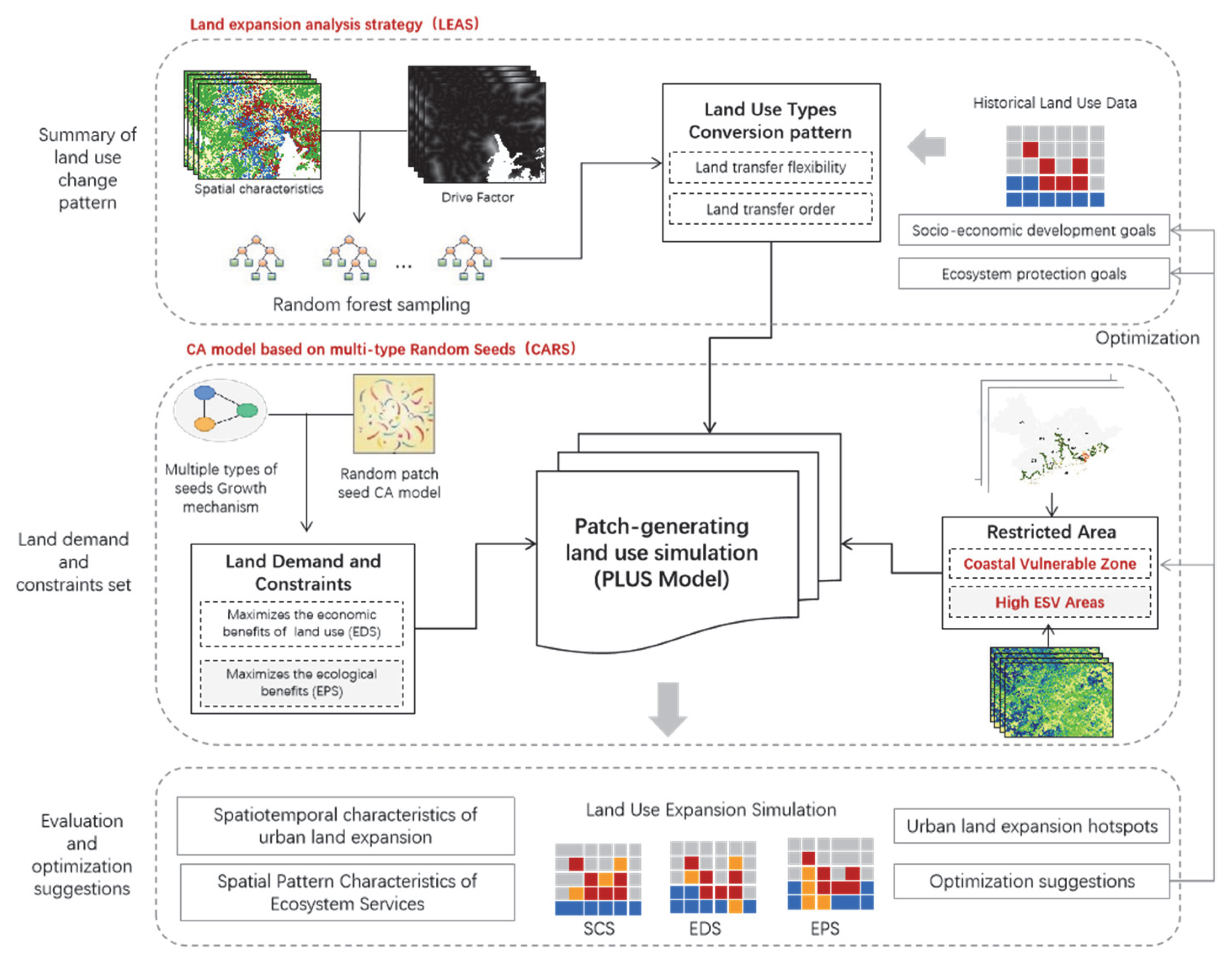
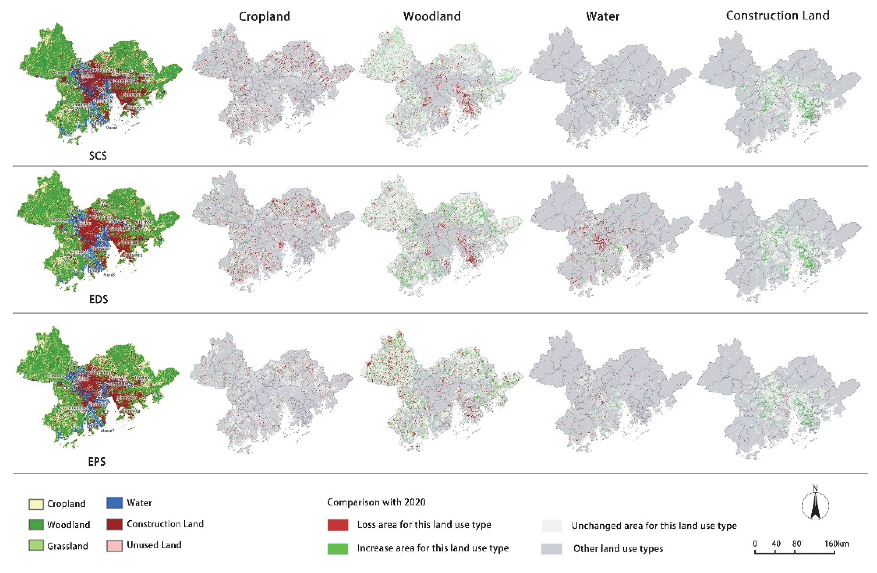
SCS maintains the current urban development concept and follows the historical development law, using historical land use data to forecast the area of each land use type in 2035.
EDS maximizes the economic benefits of each land use type to satisfy the ecological and population carrying capacity.
S 2 ( l ) = i = 1 6 Eco i × l i
where S 2 ( l ) is the sum of economic benefits of each land use type, and index I represents land use type i = 1, 2,…, 6, indicating cropland, woodland, grassland, water, construction land, and unused land; I is the economic benefits generated per unit area of the different land use types. The economic efficiency coefficients of the GHM-GBA were set based on the historical data from the Guangdong Provincial Bureau of Statistics (2001–2016). The total production value of agriculture, forestry, livestock, and fishery was used to estimate the economic benefits of cropland, woodland, grassland, and water, respectively. The GDP of the secondary and tertiary industries can be used as a proxy for the economic benefits of the construction land. Equation (2) can be rewritten as follows:
S 2 ( l ) = 19.44 l 1 + 1.10 l 2 + 31.94 l 3 + 22.76 l 4 + 1122.87 l 5 + 0 l 6
EPS adopts ecological carrying capacity to measure ecological benefits, maximizes the ecological benefits provided by different land use types, strictly protects areas with high ES effectiveness, and appropriately limits economic growth.
S 3 ( l ) = i = 1 6 Ec i × l i × ( 100 12 ) % = i = 1 6 Q i × Y i × l i × 88 %
In this paper, the ecological equilibrium factors for cropland, forest, grassland, watershed, construction land, and unused land were 2.49, 1.28, 0.46, 2.49, 0.37, and 1.28, respectively [36]. The yield factors were set to 1.94, 1.18, 0.81, 1.66, 1.27, and 0.00, respectively, according to the average yield factor in China. There is a requirement of reserving 12% of land for biodiversity conservation. The adjusted function can be expressed in Equation (4):
S 3 ( l ) = 4.83 l 1 + 1.51 l 2 + 0.37 l 3 + 4.13 l 4 + 0.47 l 5

3.2. Parameter Setting for PLUS Model

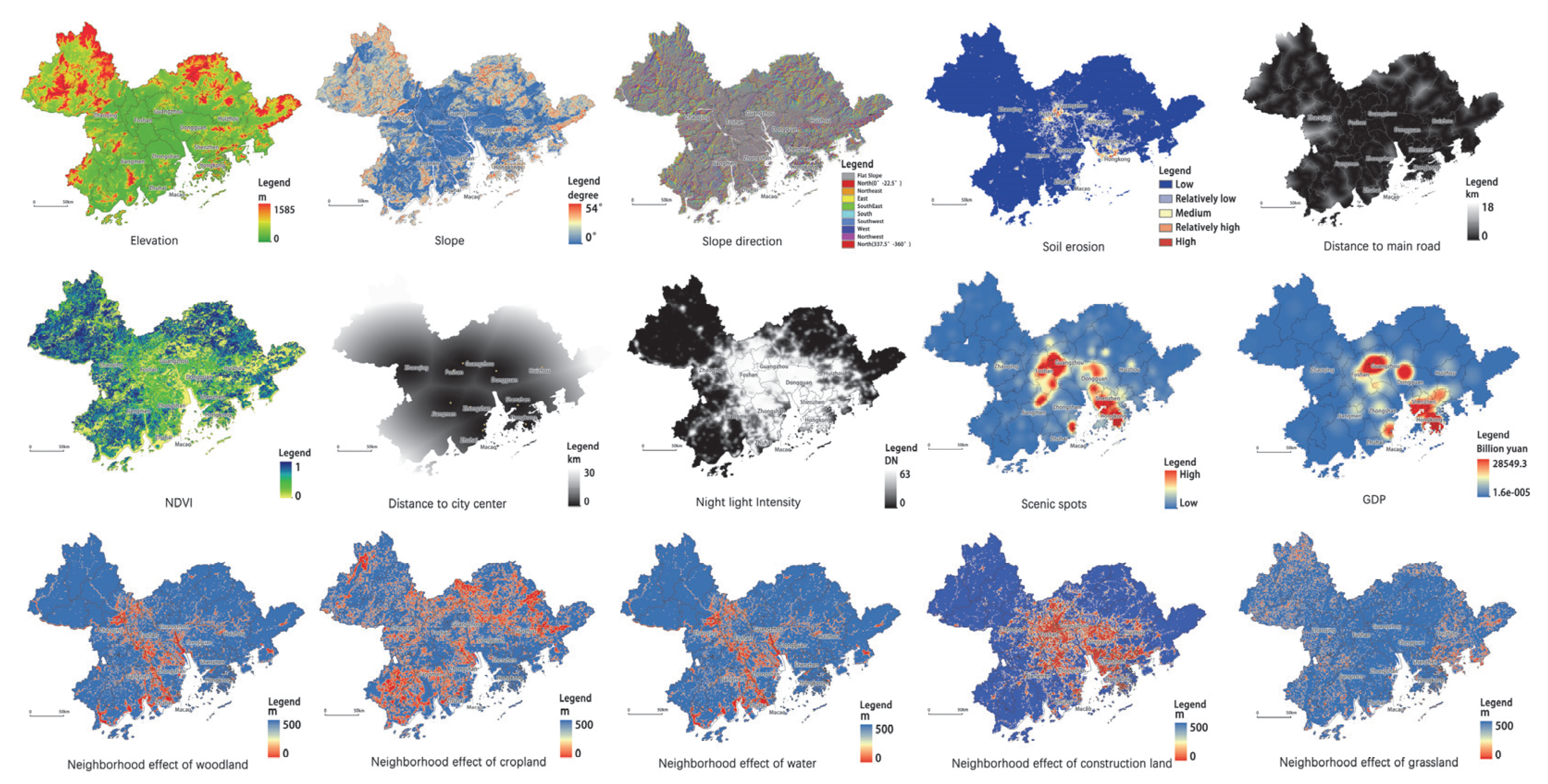
The drivers characterize specific land use suitability as influenced by physical and socioeconomic factors and play a dominant role in modeling future land expansion trends. First, the study selected 12 drivers to import into a random forest model to extract the high-level semantics of urban suitability for different land use type transitions (Figure 5).
Second, the land use conversion rules included the neighborhood parameter and the land use conversion cost matrix. The neighborhood parameter indicated the ease of land use type conversion, and higher values indicated that the land use type was less likely to occur. We defined this parameter based on the land use transfer rate between 2000 and 2020. Therefore, the neighborhood parameters were set as 0.8, 0.6, 0.5, 0.7, 0.9, and 0.2 for cropland, woodland, grassland, water, construction land, and unused land, respectively. The conversion cost matrix expressed the conversion cost between land types. Considering the actual situation and referring to the status quo statistics, the SCS setting allowed conversion among all land types. In contrast, the EDS and EPS settings did not allow the conversion of cropland, woodland, and construction land to unused land.
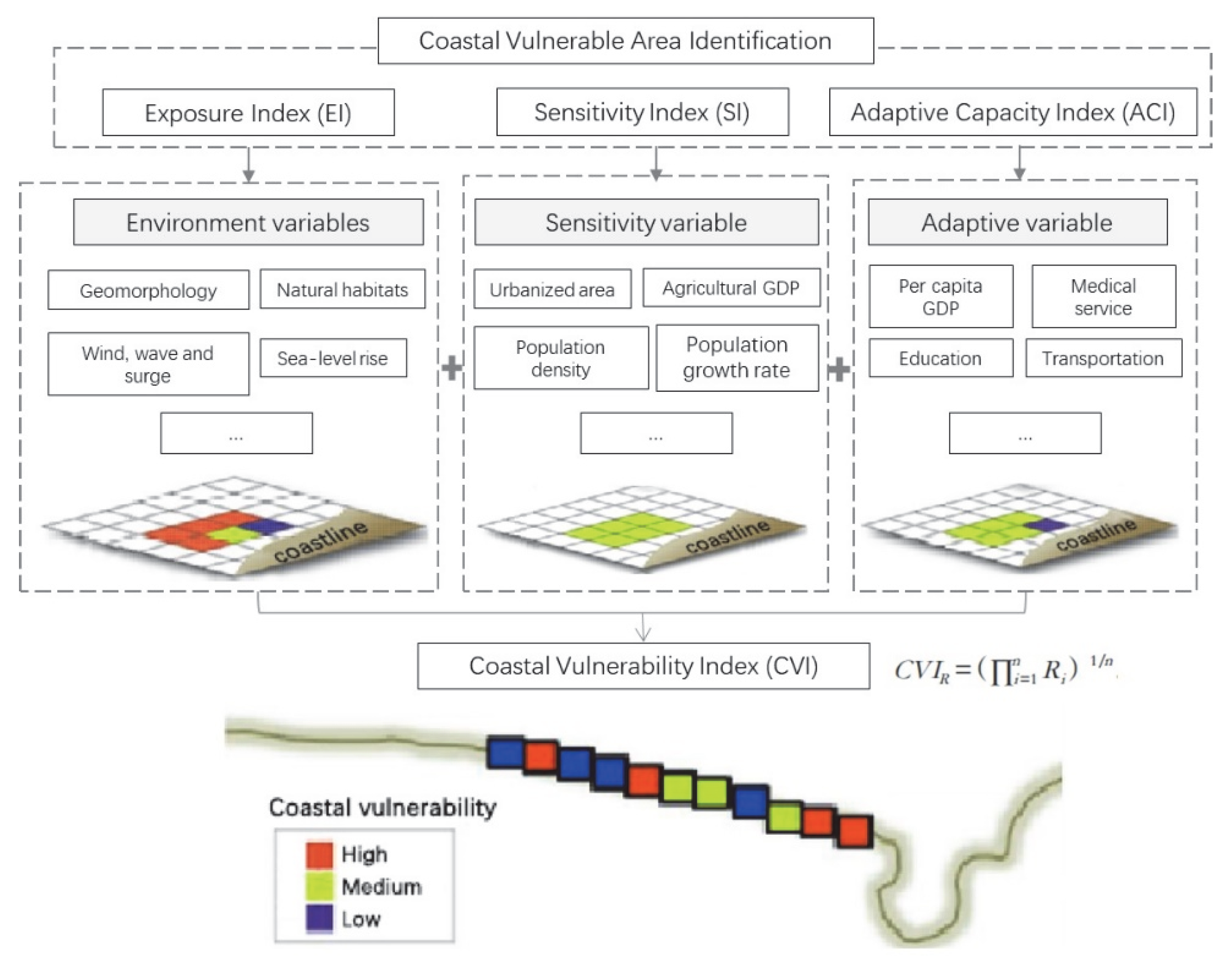
Third, based on a combination of historical data and planning information, we set separate projections for the future scale of demand for each type of site. SCS used Markov Chain to predict the quantitative relationship of each type of land in 2035, and the total land scale of EDS and EPS was consistent. The other constraints were set separately by combining the planning objectives with the land use economic efficiency (Formula (1)) and ecological efficiency (Formula (3)). The optimal solution for land demand was obtained by Python linear programming code calculation. At the same time, we set strict protection areas for EDS. We set the calculation indexes and classification criteria for ES effectiveness and vulnerable coastal zone, respectively (Table 2). We extracted high-ESV areas and highly vulnerable coastal zones with the ArcGIS reclassification function. Then, we realized the aggregation and integration of two types of restricted areas by overlay analysis. The land use of these areas was set to not be converted to construction land.
Finally, we imported the above parameters and the land use data of the GHM-GBA into the PLUS model and used the land use data from 2000 to 2020 for historical testing and optimization. The Kappa coefficient of the model was 0.84, and the overall accuracy was 89.6%, indicating that the model had high accuracy in simulating land use changes in urban agglomerations. The simulation results will guide spatial planning decisions.

3.3. Methods for Quantifying Land Use Change Patterns

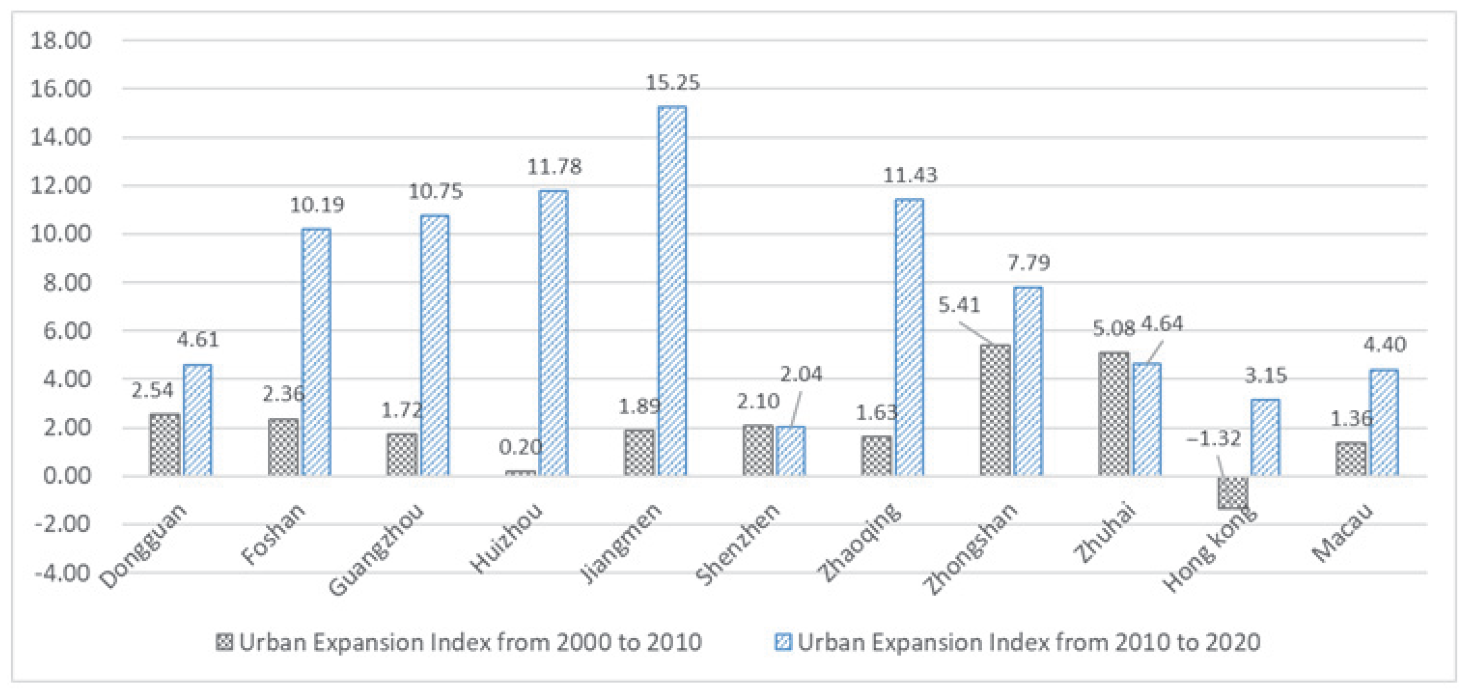
The urban expansion index (UEI) can reflect the degree and speed of land expansion within a specific time interval [37]. This study used UEI to measure the temporal changes in land expansion in the GHM-GBA. The calculation formula is as follows:
UEI = A n 1 A n 2 A n 1 × Δ n × 100 %
where UEI represents the intensity of urban land expansion; A n 1 and A n 2   represent the area of urban land in years n1 and n2, respectively; Δ n   is the interval time in years.
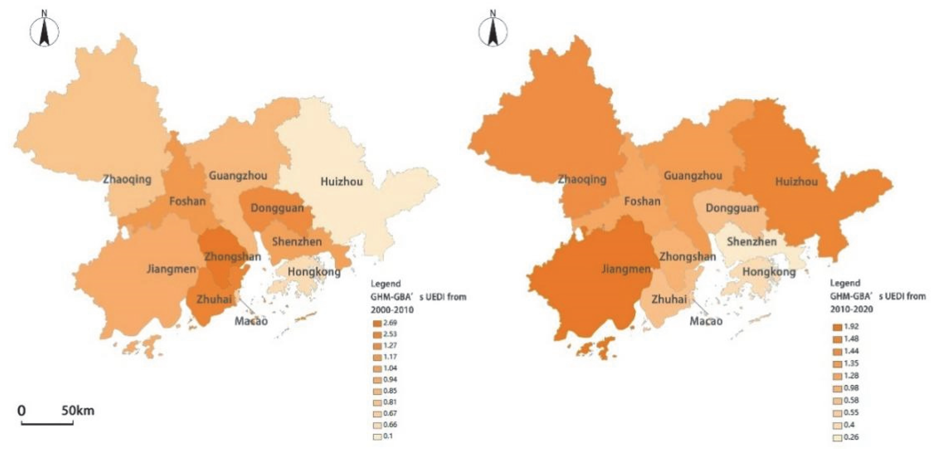
In addition, the land expansion trend of each city varied depending on the spatial elements, positioning, and development context. In order to exclude the influence of city size and further clarify the differences in expansion intensity among cities in the GHM-GBA, the Urban Expansion Difference Index (UEDI) was used to characterize the differences in land expansion. The formula is:
UEDI = ( A n 2 A n 1 ) × UA n 1 ( UA n 2 UA n 1 ) × A n 1 × 100 %
where UEDI represents the land expansion disparity index; A n 1   and   A n 2 represent the construction land area of individual cities in years n1 and n2, respectively; UA n 1 and UA n 2 represent the total construction land area of urban agglomerations in years n1 and n2, respectively.

3.4. Methods for Analyzing Spatial Patterns of ES and ESV

We used the Chinese terrestrial ES unit area service value equivalent to calculate ESVs to quantify ES effects in the three scenarios. Since the unit ESV equivalents estimated in developed countries do not reflect the “willingness to pay” of people in developing countries for ecosystems, Xie et al. improved the Costanza et al. ESV unit cost coefficients [12,38]. After combining two surveys of 700 Chinese ecologists, they developed a Chinese ESV equivalent scale. We followed that data and corrected it with the spatial heterogeneity of ES. To visualize the spatial pattern of ESVs, ES in this study were calculated using a spatial resolution of 90 m × 90 m.
Evaluation of ES at the spatial scale should also consider the spatial heterogeneity of ES in different land use types [39]. Established studies have shown that ES is positively correlated with vegetation cover type and biomass. Hence, the study chose to reflect the spatial heterogeneity of ES by calculating the carbon sink value in terms of carbon storage [40]. Carbon stock (CS) is the sum of aboveground organic carbon ( C above ), belowground biomass organic carbon ( C below ), soil organic carbon stock ( C soil ), and organic carbon in apoplastic matter ( C dead ) in an ecosystem [41,
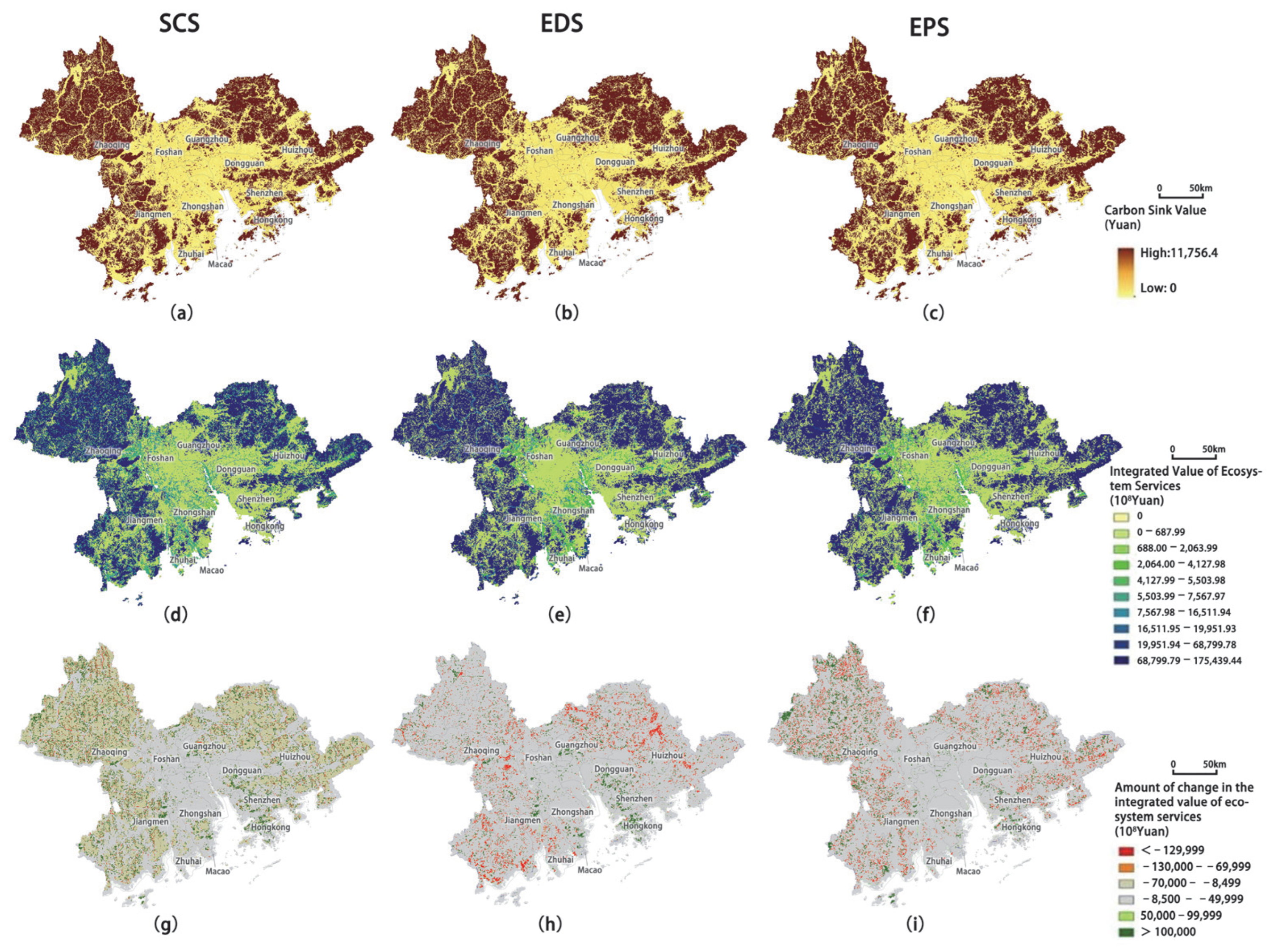
42]. Therefore, this paper adopted the Carbon Storage and Sequestration: Climate Regulation module in the InVEST model to calculate the ecosystem carbon storage and used the first carbon trading price in China (CNY 52.78/ton) as the unit price to calculate the carbon sink value, and finally measured the comprehensive ESV results. The calculation formula is as follows:
ESV = j = 1 6 a × E ij × CS i × 52.78
where ESV is the integrated ecosystem service value, index i represents land use type i = 1, 2,…, 6, indicating cropland, woodland, grassland, water, construction land, and unused land; E ij is the economic benefit derived from the unit area of the different land use types. CS i represents the total carbon stock and is calculated by the formula:
CS i = C above + C below + C soil + C dead
where C above ,   C below ,   C soil ,   C dead represent aboveground carbon stock, belowground carbon stock, soil carbon stock, and dead biological carbon stock, respectively.

4. Results

4.1. Step 1: Summary of Land Use Change Pattern

Figure 6 shows that, since 2010, the urbanization development of the GHM-GBA has accelerated significantly. From 2000 to 2010, Zhongshan had the highest UEI at 5.41%, followed by Zhuhai and Dongguan with 5.08% and 2.54%, respectively. From 2010 to 2020, Jiangmen City, Huizhou City, and Zhaoqing City and other node cities showed urban development with UEI values of 15.25%, 11.78%, and 11.43%, respectively. As the geometric center of the GHM-GBA and the important transportation hub in the future, Zhongshan City has risen rapidly with the help of the construction of major regional transportation infrastructures, such as the Hong Kong–Zhuhai–Macao Bridge and the Shenzhen–Maoming Railway.
Applying the UEDI index to measure the difference in urban spatial expansion in the GHM-GBA showed a significant difference in the expansion intensity of different cities and an uneven pattern of urban spatial expansion in the study area (Figure 7). During 2000–2010, from the overall spatial distribution, the cities with high urban spatial expansion were concentrated in the central part of the urban agglomeration. The urban spatial expansion difference indices of Zhongshan, Zhuhai, and Dongguan were significantly higher than the urban agglomeration average of 1.16, especially the UEDI index of Zhongshan, which was 2.69. The urban construction land increased from 235.22 km2 in 2000 to 362.58 km2, experiencing a rapid urbanization development higher than the overall level of the GHM-GBA. Other cities’ urban land expansion rates were lower than the average of urban agglomerations, with values ranging from 0.1 to 1.04. During 2010–2020, the overall spatial distribution differed from the previous period, with the distribution of cities with high urban space expansion gradually expanding from coastal to inland; Jiangmen, Huizhou, and Zhaoqing showed strong urban land expansion, with UEDI indices of 1.92, 1.48, and 1.44, respectively. Jiangmen City had the most noticeable increase in construction land, from 315.79 km2 in 2010 to 797.34 km2 in 2020, with nearly 1.5 times the new construction land area. The construction land area of Zhaoqing increased from 268.31 km2 in 2010 to 575.09 km2 in 2020. The average level of urban agglomeration was also lower than the previous period, with a UEDI index of only 0.98. The UEDI of Foshan coincided with the average level of urban agglomeration, and the UEDIs of Dongguan, Huizhou, and Jiangmen were all lower than the average urban agglomeration level.

4.2. Step 2: Land Demand and Constraints Set for EDS and EPS

4.2.1. Land Demand, Demand Analysis, and Formula

The total area did not change, and we set the sum of land use area types in the three scenarios equal to the total land use area of the GHM-GBA (56,972 km2). Based on the population growth rate from 2015 to 2020, the upper limit of the population number in 2035 was set to 120 million people. Other land demands are shown in Table 3.

4.2.2. Restricted Area

The construction land has expanded greatly, increasing by about 115% in the last 20 years. The spatial distribution of ESV variation showed a “high center, low periphery” pattern of loss. The regions where a higher degree of ESV gains occurred were mainly located in Jinwan District, Zhuhai, and Dinghu District, Zhaoqing, where higher values of regulation and supply services were obtained owing to the transfer of a small amount of cropland to the water (Figure 8). The high-value areas of ESV loss were concentrated in Foshan City and Shunde District, the coast of Jiaoyi Bay in the Pearl River Estuary, the Cotai Reclamation Area in Macau, and the Gaolan Port Economic Zone in Zhuhai. It was not difficult to determine that these areas were in the water-rich land and water ecological transition zone. During the 20 years of rapid urban development, urban construction activities in these areas encroached on ecological lands, such as high-intensity lake enclosure and land reclamation, resulting in conversion of a large amount of ecological land with high ESVs to construction land. Larger areas of medium to low ESV loss occurred in Guangzhou and Dongguan, where the transfer out of forest and water areas and the transfer in of cropland and construction land were the leading causes of ESV loss. It is worth noting that, as one of the most densely populated regions in the world, Hong Kong has scarce land resources. However, its total loss in the last two decades has been minimal, and some areas have even experienced ESV gains. This was due to the strict legislative protection policy for ecological space in effect since the 1970s. Its vegetation cover and biomass were much higher than those of other cities of the GHM-GBA. Nearly 40% of the land still belonged to forest parks, where ES were fully utilized within the limited land resources. We extracted high ES areas and coastal high vulnerability areas through the ArcGIS reclassification function, and set this area as restricted area (Figure 9).

4.3. Step 3: Land Expansion Simulation

4.3.1. The Pattern of Land Expansion of Predicted Scenarios

The land use type of the GHM-GBA was dominated by forest, followed by cropland and construction land. In 2020, the area of forest had the highest proportion (48.1%), followed by cropland (18.8%) and construction land (16.9%). The simulation results indicate that forest, cropland, and grassland area all showed a decreasing trend from 2020 to 2035 (Table 4). A comparison of land use changes under the three scenarios showed a significant increase in construction land between 2020 and 2035, with EDS showing a much higher rate of construction land expansion than SCS and EPS (25% increase relative to 2020). Since construction land expansion comes at the expense of other land types, cropland and grassland were the land types with the most extensive area loss of all scenarios. Comparing the EDS and EPS scenarios indicated the importance of ecological conservation policies in controlling urban sprawl: the EPS scenario had a relatively stable area of grassland and forest and a low rate of cropland contraction. The EDS showed a significant loss of water area and cropland area, with the extensive loss of water area occurring around the East China Sea waterway and the Xijiang River fork of Zhongshan City, and the immense loss of cropland area occurring mainly in Nansha District, Guangzhou City, and Boluo County, Huizhou City (Figure 10).

4.3.2. Ecosystem Services Characteristics of Predicted Scenarios

The ESV changes from 2020 to 2035 were calculated based on land use types and the ecosystem service equivalent value per unit area (Table 5). The results showed that climate regulation and hydrological regulation were the two dominant ES in the GHM-GBA, accounting for 24% and 37% of the total ESVs in 2020, respectively (Table 6). Between 2020 and 2035, all the ESVs exhibited different degrees of loss, except for water supply, with the food supply function declining the most (−4.07%). A cross-sectional comparison of the three scenarios showed that EDS had the highest ESV loss, with a 3.05% decrease compared to 2020, followed by SCS (2.89%) and EPS (1.33%). The continued urban expansion in the GHM-GBA has already had a profound negative impact on ES, which could lead to a total ESV loss of USD 28.1 billion in 2035 if an economic-first development model is adopted.
In terms of spatial layout, Figure 11a–c shows the carbon sink values of SCS, EDS, and EPS, among which the carbon sink values of EPS were generally higher and more compactly distributed in the region, which is essential for protecting the overall carbon balance and ecosystem stability of the construction area. In areas such as Baiyunshan Scenic Area in Guangzhou, Dalingshan Forest Park in Dongguan, and woodlands on both sides of Provincial Road 262 in northern Zhaoqing, the carbon sink values of EPS were significantly higher than those of other scenarios, indicating that the EPS helped to maintain the carbon stocks of different land uses at a high level. It is worth noting that, although the land area of Hong Kong is small, accounting for only 2% of the area of the GHM-GBA, its carbon storage per unit area is much higher than that of Guangzhou, Shenzhen, Dongguan, and other cities. This is due to the fact that Hong Kong has protected about 40% of the total forest park area through legislation since the 1970s. The vegetation coverage and biomass are much higher than those of other cities, so the advantage of carbon storage is obvious. ESV distribution generally showed a more apparent spatial heterogeneity, with relatively high ESVs in the ecological barrier areas in the northeast and west wings of the GHM-GBA, corresponding to the vital node cities of Zhaoqing, Jiangmen, and Huizhou (Figure 11d–f). The spatial layout characteristics of the integrated ESV gains and losses of the three scenarios differed significantly: SCS showed a large area of low to moderate ESV loss attributed to the transformation of some woodland to cropland and construction land. In addition, because of physical geography and forest age structure, the carbon initially stored in woodland was released into the atmosphere, and forest carbon stocks were significantly reduced, resulting in a total ESV loss. Figure 11g–i indicates the spatial agglomerations with severe ESV losses in the EDS scenario distributed along the highways or urban fringe areas in Boro County, Huizhou City, eastern Taishan City, and Foshan City.

4.4. Analysis of the Interaction between Urban Land Expansion and Ecosystem Services

4.4.1. Correlation of Urban Land Expansion Drivers with ESVs

Table 7 illustrates that gas regulation and climate regulation services were significantly correlated with various factors. The value of areas with lower population density, far from roads and gentle terrain, tended to be higher. Areas with a high value of soil support were usually located in areas with low population density and far from main roads. Areas with a high value of biodiversity and recreation culture were located in areas with high soil quality, good vegetation cover, and far from main roads. Areas with high values of water supply and food supply were located in areas with high soil quality and far from main roads and city centers. High-value areas for biodiversity and recreation were located in areas with high soil quality, good vegetation cover, and far from main roads. High-value areas for water supply and food supply were located in areas with high soil quality and far from main roads and city centers. The urbanization element showed the most apparent depletion of ESVs and became the main driver of the decline in each individual ESV.

4.4.2. Analysis of Urban Land Expansion Hotspots and ESV Correlation

Based on the simulation results under different land use scale conditions, the priority expansion directions and locations of future urban land development in the GHM-GBA were analyzed (Figure 12). By extracting the overlapping areas of construction land under the three scenarios to identify hotspots of urban land expansion, the results indicated that urban construction land showed a trend of expansion to the southeast. These areas will experience rapid urbanization in 2020–2035. By 2035, Shenzhen’s Guangming District and Futian District will have expanded significantly, followed by Jiangmen’s Pengjiang District, Dongguan City, and Zhuhai’s Xiangzhou District. New construction land often appears at the edge of urban and rural residential areas, converted from cropland and forest to construction land. Owing to differences in geographic, natural, and socioeconomic conditions, the expansion hotspots showed different patterns of construction and expansion, such as “infill expansion” in Shunde District in Foshan City; “outward expansion” in Yuexiu District in Guangzhou City and Futian District in Shenzhen City; and “leapfrog expansion” in Dongguan City. In addition, overlaying the spatial pattern of construction land expansion hotspots and ESVs, we found that the construction land expansion hotspots in Shatin, Zhaoqing City, and the Xiangzhou District of Zhuhai are likely to encroach on high-ESV land. For such critical areas of the economic–ecological game, it is important to promote renewal of urban stock resources, such as the redevelopment of shantytowns and abandoned factories, to avoid the disorderly spread of urban construction land encroaching on high-quality cropland and woodland.

5. Discussion and Conclusions

5.1. Discussion

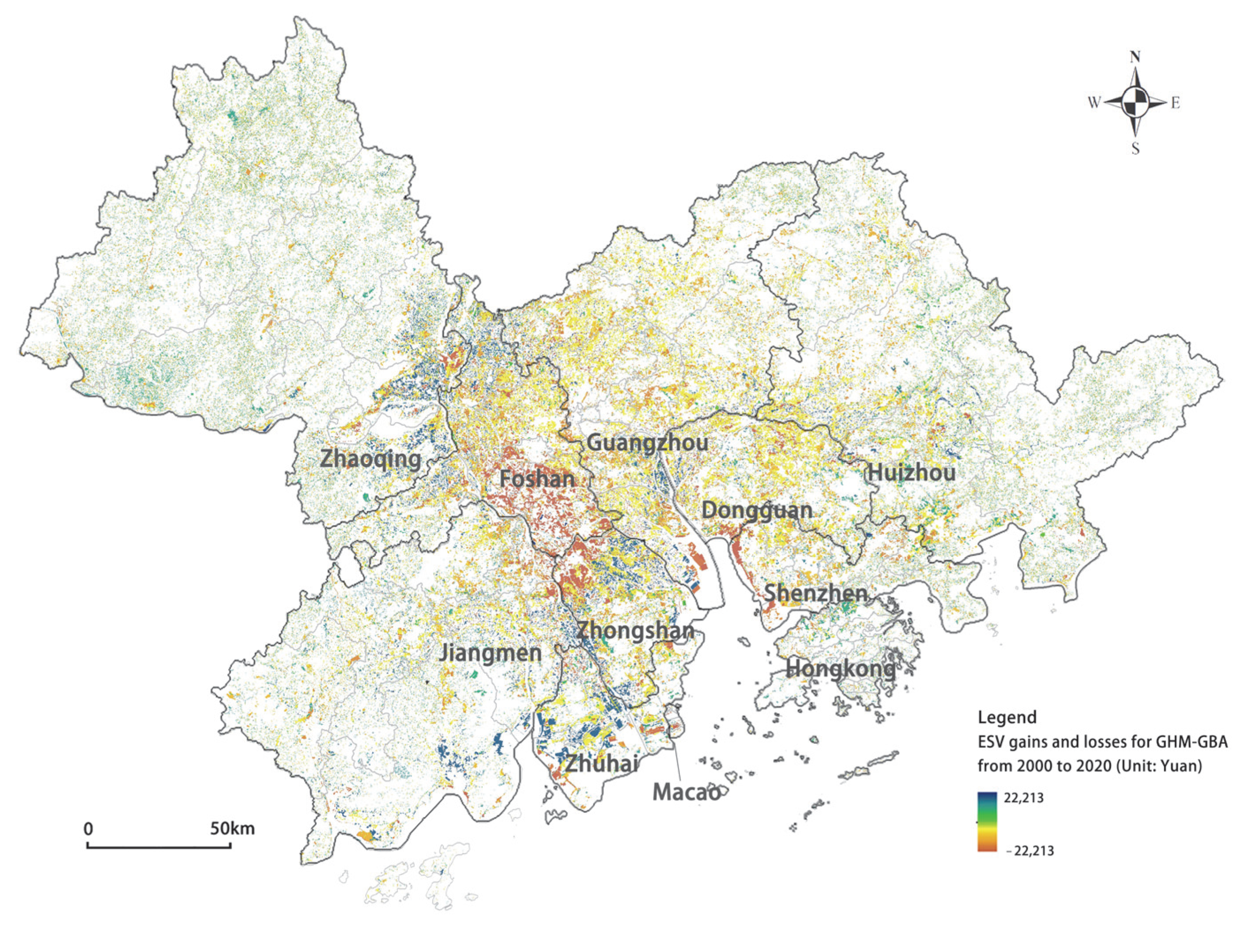
In the last two decades, the ecological land area in the Greater Bay Area has experienced significant declines, with the highest decline in cropland (−22.5%), followed by grassland and forest at −14.98% and −3.7%, respectively. Most of these ecological lands were converted to urban construction land, thus leading to a significant loss in ecosystem services. Compared with S1, the loss of cropland and forest land in S2 is not significant; however, a large area of grassland and water is converted to urban construction land, and these two types of land also provide considerable ESV. Therefore, the focus should be on protecting grassland and water areas in the GMH-GBA construction hotspot. Specifically, ideal land use planning should be addressed in the following discussion, with methods, results, and optimization strategies.

5.1.1. Simulation of Land Expansion from the Ecosystem Services Perspective Provides a Unified Perspective

The ES-perspective-based land expansion simulation method provided a unified perspective on natural resource status, spatiotemporal trade-offs and synergistic effects, and human welfare for the ecological spatial classification system, optimizing land development patterns and regulating spatial order. The multi-scenario land expansion simulation model constructed in this paper can provide a basis for preparation of spatial planning in ecological civilization construction and strengthen the consensus on the ecological bottom line in urban planning. In the GHM-GBA case study, the modified ES equivalent and carbon sink values can effectively reflect the integrated ESV spatial heterogeneity, which can be used as an entry point to realize the multidisciplinary cross-coupling of ecosystems and social systems. In current ES quantification studies, ESVs are primarily measured based on the equivalent coefficients of land use types. Talukdar et al. (2020) classified LULCs in the lower Gangetic plain of India into six categories and calculated ESV values by multiplying the sum of land use area with the ESV of that LULC type, showing that the area of water decreased by 15% and the ES provided by water have decreased accordingly. Land use has changed over the last decade, so the ecosystem service values have also changed [43]. Mendoza-González et al. (2012) used a benefit transfer approach to calculate ESV using land use changes and found that land use changes increased economic benefits but lost ES, such as coastal protection or scenic values [44]. However, the same land use type often carries multiple ES, and quantification of ESVs by land use type alone ignores the spatial heterogeneity and is prone to ES measurement homogenization. Compared with other studies, this study adopted the carbon storage module of the InVEST platform, which combines the traditional ESV calculation method with carbon sink value. It comprehensively evaluated the ESV distribution spatial pattern under different urban development scenarios. The technical approach can build a comprehensive data platform for ecological structures, processes, services, and benefits, enhance the monitoring technology of ecological environment and socioeconomic attributes, help to achieve China’s carbon peaking and carbon neutrality goals, and provide a reference for regional “bottom-up” spatial planning and high-quality urban development.

5.1.2. Multiple Scenario Simulation Results: A possible Optimal Path to Realizing Ecological Civilization

The coupling of multi-objective linear planning of land scale prediction and the PLUS model of urban land expansion simulation analysis scientifically allocated the “quality” value of ecosystems and the “quantity” of natural resources. Previous studies on land expansion have mainly set constraints and predicted land use scale based on historical data or empirical values. In contrast with other studies, Das et al. (2022) used CA-Markov models to predict land use land cover and the causes of ecosystem service change in the Kolkata urban agglomeration by 2040 [45]. Barred and Demicheli (2003) proposed a bottom-up approach that combines land use factors with a dynamic approach to simulate land use scenarios in Lagos, offering the possibility of exploring future spatial patterns of land use under specific assumptions [46]. Chang and Ko (2014) developed an interactive dynamic multi-objective planning (IDMOP) model to derive compromising quantitative land use optimization solutions that balance the conflicting objectives of various stakeholders [47]. However, GHM-GBA is in the stage of rapid land use expansion, and the guidance of its land use planning should not be limited to a single aspect of the land use scale quantitative optimization or land use spatial pattern. In other words, focusing only on the quantity of land use type cannot allocate land use to the ideal location, and focusing only on the spatial pattern may lead to a land use scale that cannot meet the needs of ecological protection and economic development. Therefore, the coupled model constructed in this study integrated the “top-down” and “bottom-up” perspectives, which optimized the scale and spatial pattern of various land uses from the ES perspective. First, the essence of the MOP algorithm was to seek the optimal structural effect of land use. Simulating a top-down macroscopic decision-making process optimized allocation of various land use scales under a series of socioeconomic and ecological constraints to achieve the specific purpose of maximizing economic or ecological objectives under three scenarios of constraints. Second, the PLUS model allocated the predicted land use demand to the most appropriate spatial location and participated in the spatial development and restriction policies according to a bottom-up process to achieve an intersection of land use scale and spatial pattern. According to the prediction results of the coupled model, EPS improved the spatial agglomeration of ESVs and construction land in urban agglomerations. It promoted the “win–win” situation of high-quality economic development and high-level ecological environment protection. In addition, the research results provided various simulation scenarios for urban land expansion by combining climate change and ES as the basis for delineating the control lines of ecology, agriculture, and urban function space. Based on the relationship between ES and urban land expansion, we explored the framework of spatial planning methods from the perspective of ES and the preferred path to realize ecological civilization.

5.1.3. Land Use Optimization Strategies for Urban Agglomeration in the GHM-GBA Based on Simulation Results

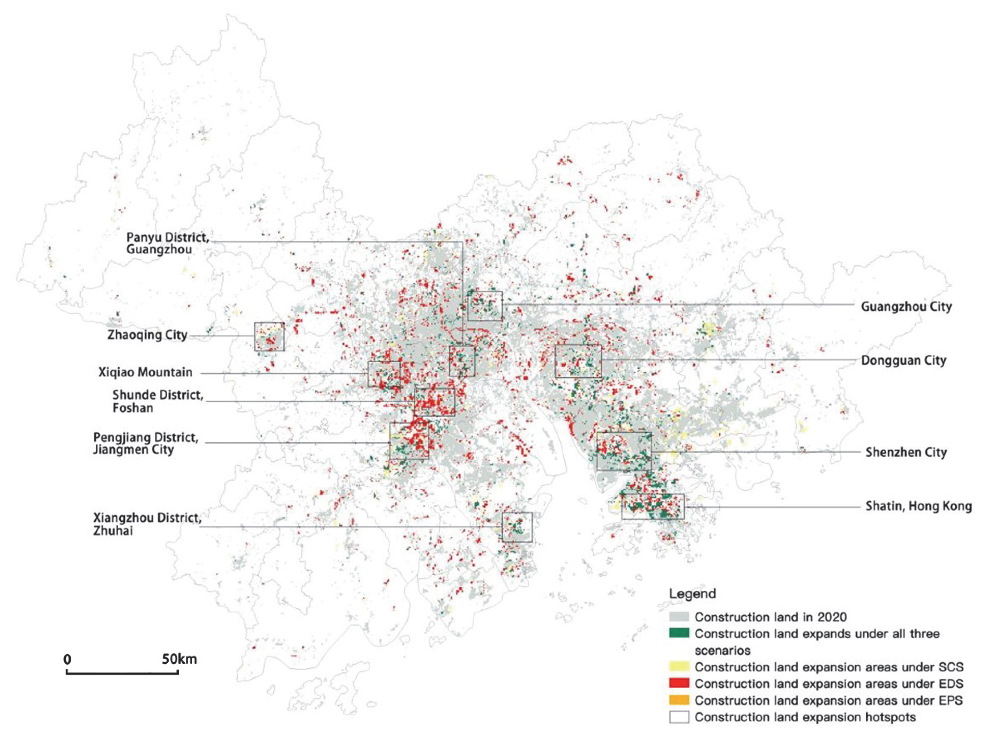
China’s territorial spatial control focuses on strategic (conceptual) content, with a preference for top-down decomposition and transmission of indicators, such as target goals and policy content. One of the strengths of ES is representation of ESV variation patterns on spatial and temporal scales, thus revealing the dual role of constraints and guidance between ES and land resource allocation. Therefore, the coupled model provided a research basis for realizing multidimensional, multi-objective, and multi-level urban growth management. The research results revealed the hotspots of urban construction land expansion in the ecological–economic game process, and we proposed corresponding optimization strategies, including focusing on efficient use of urban stock resources in high-ESV areas, such as Zhaoqing City and Xiangzhou District, promoting transformation of traditional passive defenses of ecological space into active restraint, and, finally, realizing a comprehensive management path of land use. In terms of planning strategies, Guangdong has launched several new ecological protection plans, including the Guangdong Province Climate Change Response Program and the Pearl River Delta National Forest City Cluster Construction Plan, effectively restoring degraded ecosystems. However, the proposed target of carbon emission intensity reduction in the GHM-GBA brings enormous pressure and challenges. Thus, predicting future land use changes and their possible impacts on ecosystems under different development scenarios can help to address the challenges. Based on the above background, differentiated planning optimization suggestions were made for each city in the GHM-GBA: (1) an adjustment-type policy was proposed for the three high-quality ES areas of Zhaoqing, Jiangmen, and Huizhou. As the ecological barrier of the study area, it has high forest cover and carbon storage levels and should adjust the boundary line of cropland protection and ecological protection. It should adopt strict protection policies according to the ES prediction results and control urban expansion to guarantee the primary source of carbon storage in the GHM-GBA. (2) Guideline policies should be formulated for the highly urbanized areas of Guangzhou, Shenzhen, Hong Kong, and Macao. This study found that high-ESV areas easily encroached on by urban land were mostly located in and around urban built-up areas. We recommend optimizing the quality of green areas in built-up areas based on safeguarding the existing ecological environment quality to enhance ES and guide formation of ecological corridors within a limited area. (3) A controlled policy should be formulated for Foshan, Zhongshan, Zhuhai, and Dongguan regions. They must improve the construction of multi-level green space systems within the cities, strengthen the implementation of natural resource protection planning and spatial regulations in the urban–rural combination areas, and strictly control cropland conversion to other land types.

5.1.4. Study Limitations

The present study still has the following shortcomings, which need to be explored more deeply in the future: this study focuses on land use planning theories, methods, and optimization strategies at the macro urban agglomeration scale. In the future, we should continue to promote multi-scale land use spatial evolution processes and mechanisms, form a multi-spatial-scale integrated decision-making toolbox, and improve the land use planning and optimization system under the perspective of ecosystem services.

5.2. Conclusions

Against the background of natural resource scarcity, a consensus to explore the balance between urban development and ecological protection has been reached. This paper integrated the research methods of ES assessment, coastal vulnerability evaluation, multi-objective linear planning, and land use change simulation and constructed a multi-scenario urban land expansion simulation model framework from the perspective of ecosystem services. Using the Guangdong–Hong Kong–Macao Greater Bay Area as the research object, the framework was applied to simulate the spatial and temporal evolutionary characteristics of land use changes and ecosystem service values under the three scenarios of status quo continuation, economic development, and ecological protection. The results of the land use simulation indicated that the scale of construction land under the three scenarios will grow significantly. Cropland and grassland were the types of land with the most significant losses. The continued urban expansion in the GHM-GBA has already had a profound negative impact on ecosystem services. If an economic-first development model is adopted, it could result in a total ESV loss of CNY 28.1 billion by 2035. Shenzhen Guangming District and Futian District, Jiangmen Pengjiang District, Dongguan City, and Zhuhai Xiangzhou District will become hotspots for land expansion in 2035. Because of differences in geographic, natural, and socioeconomic conditions, the expansion hotspots showed different patterns of built-up expansion, such as “infill expansion” in the Shunde District of Foshan City, “outward expansion” in the Yuexiu District of Guangzhou City, and, in Dongguan City, “leapfrog expansion”. In addition, new construction land often appeared at the edge of urban and rural residential areas, converted from cropland and woodland, for which spatial regulation of land use should be enforced to prevent potential disorderly urban expansion. The multi-scenario urban land expansion simulation framework from the perspective of ecosystem services scientifically allocates the “quality” value classification of ecosystems and “quantity” stock allocation of natural resources and provides a reference for regional “bottom-up” territorial spatial planning.

Author Contributions

Conceptualization, J.W. and T.C.; methodology, J.W.; software, J.W.; validation, J.W. and T.C.; formal analysis, J.W.; investigation, J.W.; resources, T.C.; data curation, T.C.; writing—original draft preparation, J.W.; writing—review and editing, T.C.; visualization, J.W.; supervision, T.C.; project administration, T.C.; funding acquisition, T.C. All authors have read and agreed to the published version of the manuscript.

Funding

This research was funded by International Cooperation and Exchange of the National Natural Science Foundation of China, grant number 52061160366; Fundo para o Desenvolvimento das Ciências e da Tecnologia, grant number 0039/2020/AFJ; The national Natural Science Foundation of China (NSFC), grant number 52078329.

Data Availability Statement

The sources and preprocessing of data can be found in Section 2.3 and Section 3. Other data to support this research are available from the authors upon request.

Conflicts of Interest

The authors declare no conflict of interest.

References

  1. Mooney, H.; Larigauderie, A.; Cesario, M.; Elmquist, T.; Hoegh-Guldberg, O.; Lavorel, S.; Mace, G.; Palmer, M.; Scholes, R.; Yahara, T. Biodiversity, climate change, and ecosystem services. Curr. Opin. Environ. Sustain. 2009, 1, 46–54. [Google Scholar] [CrossRef]
  2. Bai, Y.; Ochuodho, T.O.; Yang, J. Impact of land use and climate change on water-related ecosystem services in Kentucky, USA. Ecol. Indic. 2019, 102, 51–64. [Google Scholar] [CrossRef]
  3. Nelson, E.; Sander, H.; Hawthorne, P.; Conte, M.; Ennaanay, D.; Wolny, S.; Polasky, S. Projecting global land-use change and its effect on ecosystem service provision and biodiversity with simple models. PLoS ONE 2010, 5, e14327. [Google Scholar] [CrossRef] [Green Version]
  4. Garcia, S.M.; Cochrane, K.L. Ecosystem approach to fisheries: A review of implementation guidelines. ICES J. Mar. Sci. 2005, 62, 311–318. [Google Scholar] [CrossRef] [Green Version]
  5. Wang, S.; Jia, M.; Zhou, Y.; Fan, F. Impacts of changing urban form on ecological efficiency in China: A comparison between urban agglomerations and administrative areas. J. Environ. Plan. Manag. 2020, 63, 1834–1856. [Google Scholar] [CrossRef]
  6. Xu, W.; Yan, W.; Li, X.; Zou, Y.; Chen, X.; Huang, W.; Miao, L.; Zhang, R.; Zhang, G.; Zou, S. Antibiotics in riverine runoff of the Pearl River Delta and Pearl River Estuary, China: Concentrations, mass loading and ecological risks. Environ. Pollut. 2013, 182, 402–407. [Google Scholar] [CrossRef]
  7. Estoque, R.C.; Murayama, Y. Intensity and spatial pattern of urban land changes in the megacities of Southeast Asia. Land Use Policy 2015, 48, 213–222. [Google Scholar] [CrossRef]
  8. Maimaiti, B.; Ding, J.; Simayi, Z.; Kasimu, A. Characterizing urban expansion of Korla City and its spatial-temporal patterns using remote sensing and GIS methods. J. Arid Land 2017, 9, 458–470. [Google Scholar] [CrossRef] [Green Version]
  9. Ma, X.; He, S.; Huang, T.; Wang, Y. Analysis of the spatial and temporal pattern characteristics and driving factors of urban land expansion, taking the Central Plains urban agglomeration as an example. Ecol. Econ. 2020, 3, 105–111. [Google Scholar]
  10. Dutta, D.; Rahman, A.; Paul, S.K.; Kundu, A. Impervious surface growth and its inter-relationship with vegetation cover and land surface temperature in peri-urban areas of Delhi. Urban Clim. 2021, 37, 100799. [Google Scholar] [CrossRef]
  11. Burkhard, B.; Kroll, F.; Nedkov, S.; Müller, F. Mapping ecosystem service supply, demand and budgets. Ecol. Indic. 2012, 21, 17–29. [Google Scholar] [CrossRef]
  12. Xie, G.; Zhen, L.; Lu, C.; Xiao, Y.; Chen, C. An expert knowledge-based approach to valorizing ecosystem services. J. Nat. Resour. 2008, 5, 911–919. [Google Scholar]
  13. Morya, C.P.; Punia, M. Impact of urbanization processes on availability of ecosystem services in National Capital Region of Delhi (1992–2010). Environ. Dev. Sustain. 2022, 24, 7324–7348. [Google Scholar] [PubMed]
  14. Moschetto, F.A.; Ribeiro, R.B.; de Freitas, D.M. Urban expansion, regeneration and socioenvironmental vulnerability in a mangrove ecosystem at the southeast coastal of São Paulo, Brazil. Ocean Coast. Manag. 2021, 200, 105418. [Google Scholar] [CrossRef]
  15. Ouyang, Z.; Wang, X.; Miao, H. A preliminary study of terrestrial ecosystem service functions and their ecological and economic values in China. Acta Ecol. Sin. 1999, 5, 19–25. [Google Scholar]
  16. Yang, S.; Su, H.; Zhao, G. Multi-scenario Simulation of Urban Ecosystem Service Value Based on the PLUS Model: The Case of Hanzhong City. J. Arid Land Resour. Environ. 2022, 38, 86–95. [Google Scholar] [CrossRef]
  17. Li, X.; Hou, X.; Di, X.; Su, H. Exploring the ecological imbalance caused by land use change from the perspective of ecosystem services: The case of the coastal zone of Laizhou Bay. Sci. Geogr. Sin. 2016, 8, 1197–1204. [Google Scholar]
  18. Chen, Z.; Huang, M.; Zhu, D.; Altan, O. Integrating remote sensing and a markov-FLUS model to simulate future land use changes in Hokkaido, Japan. Remote Sens. 2021, 13, 2621. [Google Scholar] [CrossRef]
  19. Luo, G.; Yin, C.; Chen, X.; Xu, W.; Lu, L. Combining system dynamic model and CLUE-S model to improve land use scenario analyses at regional scale: A case study of Sangong watershed in Xinjiang, China. Ecol. Complex. 2010, 7, 198–207. [Google Scholar] [CrossRef]
  20. Okada, T.; Mito, Y.; Akiyama, Y.B.; Tokunaga, K.; Sugino, H.; Kubo, T.; Endo, T.; Otani, S.; Yamochi, S.; Kozuki, Y.; et al. Green port structures and their ecosystem services in highly urbanized Japanese bays. Coast. Eng. J. 2021, 63, 310–322. [Google Scholar] [CrossRef]
  21. Yang, C.; Li, Q.; Hu, Z.; Chen, J.; Shi, T.; Ding, K.; Wu, G. Spatiotemporal evolution of urban agglomerations in four major bay areas of US, China and Japan from 1987 to 2017: Evidence from remote sensing images. Sci. Total Environ. 2019, 671, 232–247. [Google Scholar] [CrossRef] [PubMed]
  22. Gan, L.; Chen, Y.; Wu, Z.; Qian, Q.; Zheng, Z. Changes in ecological sensitivity in the Guangdong-Hong Kong-Macao Greater Bay Area in the past 20 years. Chin. J. Ecol. 2018, 37, 2453–2462. [Google Scholar] [CrossRef]
  23. Yang, Z.; Chen, Y.; Wu, Z.; Zheng, Z. Study on the Coupling of Construction Land Expansion and Urban Heat Island Expansion in Guangdong-Hong Kong-Macao Greater Bay Area. J. Geo-Inf. Sci. 2018, 20, 1592–1603. [Google Scholar]
  24. Liu, Y.; Wang, Y.; Li, H. Implications of World-class Bay Area Industrial Development for the Construction of Guangdong, Hong Kong and Macao Greater Bay Area. Bull. Chin. Acad. Sci. 2020, 3, 312–321. [Google Scholar] [CrossRef]
  25. Liang, X.; Guan, Q.; Clarke, K.C.; Liu, S.; Wang, B.; Yao, Y. Understanding the drivers of sustainable land expansion using a patch-generating land use simulation (PLUS) model: A case study in Wuhan, China. Comput. Environ. Urban Syst. 2021, 85, 101569. [Google Scholar] [CrossRef]
  26. Hamdy, O.; Zhao, S.; Salheen, M.A.; Eid, Y.Y. Analyses the driving forces for urban growth by using IDRISI® Selva models Abouelreesh-Aswan as a case study. Int. J. Eng. Technol. 2017, 9, 226. [Google Scholar] [CrossRef] [Green Version]
  27. Chaturvedi, V.; Kuffer, M.; Kohli, D. Analysing urban development patterns in a conflict zone: A case study of Kabul. Remote Sens. 2020, 12, 3662. [Google Scholar] [CrossRef]
  28. Sharma, J.; Ravindranath, N.H. Applying IPCC 2014 framework for hazard-specific vulnerability assessment under climate change. Environ. Res. Commun. 2019, 1, 051004. [Google Scholar] [CrossRef]
  29. Vellinga, P.; Klein, R.J. Climate change, sea level rise and integrated coastal zone management: An IPCC approach. Ocean. Coast. Manag. 1993, 21, 245–268. [Google Scholar] [CrossRef]
  30. Zhang, Y.; Wu, T.; Arkema, K.K.; Han, B.; Lu, F.; Ruckelshaus, M.; Ouyang, Z. Coastal vulnerability to climate change in China’s Bohai Economic Rim. Environ. Int. 2021, 147, 106359. [Google Scholar] [CrossRef]
  31. Sathiya Bama, V.P.; Rajakumari, S.; Ramesh, R. Coastal vulnerability assessment of Vedaranyam swamp coast based on land use and shoreline dynamics. Nat. Hazards 2020, 100, 829–842. [Google Scholar] [CrossRef]
  32. Tayyebi, A.; Pijanowski, B.C.; Tayyebi, A.H. An urban growth boundary model using neural networks, GIS and radial parameterization: An application to Tehran, Iran. Landsc. Urban Plan. 2011, 100, 35–44. [Google Scholar] [CrossRef]
  33. Liu, Y.; Geng, H.; Sun, W.; Li, C.; Chu, X. Explanation to the Driving Factors for the Construction Land Expansion’s Regional Differences in the Yangtze River Delta Urban Agglomeration—Based on the Shapley Value Decomposition Method of the regression Equation. Resour. Environ. Yangtze Basin 2017, 26, 1547–1555. [Google Scholar]
  34. Xu, K.; Wu, S.; Chen, D.; Dai, L.; Zhou, S. The Urban Growth Boundary Determination Based on Hydrology Effect: Taking Xinminzhou as An Example. Sci. Geogr. Sin. 2013, 33, 979–985. [Google Scholar]
  35. Gao, L.; Tao, F.; Liu, R.; Wang, Z.; Leng, H.; Zhou, T. Multi-scenario simulation and ecological risk analysis of land use based on the PLUS model: A case study of Nanjing. Sustain. Cities Soc. 2022, 85, 104055. [Google Scholar] [CrossRef]
  36. Crop Yields. Available online: https://ourworldindata.org/crop-yields?fbclid=IwAR0-3vo_GuCC4alkWJRJcGtfv9149VHpKgk_EF9ja9P1CNV8PSl2KHpVZnI (accessed on 15 September 2022).
  37. Jiao, L.; Mao, L.; Liu, Y. Multi-order landscape expansion index: Characterizing urban expansion dynamics. Landsc. Urban Plan. 2015, 137, 30–39. [Google Scholar] [CrossRef]
  38. Costanza, R.; d’Arge, R.; De Groot, R.; Farber, S.; Grasso, M.; Hannon, B.; Limburg, K.; Naeem, S.; O’Neill, R.; Paruelo, J.; et al. The value of the world’s ecosystem services and natural capital. Nature 1997, 387, 253–260. [Google Scholar] [CrossRef]
  39. Alongi, D.M. Coastal Ecosystem Processes; CRC Press: Florida, FL, USA, 2020. [Google Scholar]
  40. Jiang, W.; Deng, Y.; Tang, Z.; Lei, X.; Chen, Z. Modelling the potential impacts of urban ecosystem changes on carbon storage under different scenarios by linking the CLUE-S and the InVEST models. Ecol. Model. 2017, 345, 30–40. [Google Scholar] [CrossRef]
  41. Li, Y.; Qiu, J.; Li, Z.; Li, Y. Assessment of blue carbon storage loss in coastal wetlands under rapid reclamation. Sustainability 2018, 10, 2818. [Google Scholar] [CrossRef] [Green Version]
  42. Nel, L.; Boeni, A.F.; Prohászka, V.J.; Szilágyi, A.; Tormáné Kovács, E.; Pásztor, L.; Centeri, C. InVEST Soil Carbon Stock Modelling of Agricultural Landscapes as an Ecosystem Service Indicator. Sustainability 2022, 14, 9808. [Google Scholar] [CrossRef]
  43. Talukdar, S.; Singha, P.; Shahfahad; Mahato, S.; Praveen, B.; Rahman, A. Dynamics of ecosystem services (ESs) in response to land use land cover (LU/LC) changes in the lower Gangetic plain of India. Ecol. Indic. 2020, 112, 106121. [Google Scholar] [CrossRef]
  44. Mendoza-González, G.; Martínez, M.L.; Lithgow, D.; Pérez-Maqueo, O.; Simonin, P. Land use change and its effects on the value of ecosystem services along the coast of the Gulf of Mexico. Ecol. Econ. 2012, 82, 23–32. [Google Scholar] [CrossRef]
  45. Das, S.; Kumar Shit, P.; Bera, B.; Adhikary, P.P. Effect of urbanization on the dynamics of ecosystem services: An analysis for decision making in Kolkata urban agglomeration. Urban Ecosyst. 2022, 25, 1541–1559. [Google Scholar]
  46. Barredo, J.I.; Demicheli, L. Urban sustainability in developing countries’ megacities: Modelling and predicting future urban growth in Lagos. Cities 2003, 20, 297–310. [Google Scholar] [CrossRef]
  47. Chang, Y.C.; Ko, T.T. An interactive dynamic multi-objective programming model to support better land use planning. Land Use Policy 2014, 36, 13–22. [Google Scholar] [CrossRef]
Figure 1. The GHM-GBA’s core cities and key node cities.
Land 11 01934 g001
Figure 2. Location of the GHM-GBA.
Land 11 01934 g002
Figure 3. Simulation model framework of urban expansion in a multi-scenario based on ES.
Land 11 01934 g003
Figure 4. Framework of coastal vulnerable area identification.
Land 11 01934 g004
Figure 5. Drive factors in the GHM-GBA.
Land 11 01934 g005
Figure 6. Urban Expansion Index of the GHM-GBA from 2000 to 2020.
Land 11 01934 g006
Figure 7. UEDI in the GHM-GBA, 2000–2020.
Land 11 01934 g007
Figure 8. ESV gains and losses for the GHM-GBA from 2000 to 2020.
Land 11 01934 g008
Figure 9. ES efficiency and coastal vulnerability spatial distribution.
Land 11 01934 g009
Figure 10. Forecast results of land expansion and changes in cropland, woodland, water area, and construction land in 2035 under scenarios S1, S2, and S3.
Land 11 01934 g010
Figure 11. (ac) Carbon sink values under SCS, EDS, and EPS scenarios; (df) the integrated ESVs; (gi) the amount of change in the integrated ESVs.
Land 11 01934 g011
Figure 12. Hotspots of built-up land expansion.
Land 11 01934 g012
Table 1. Details of all the data.
Data TypeData NameYearData ProcessingData source
Land use DataLand use type2010, 2015, 2020Classification using 30 m multispectral images.Department of Natural Resources Global Land Cover Data (http://www.globallandcover.com (accessed on 8 August 2021))
Normalized difference vegetation index2020The annual average NDVI was calculated by inversion of LANDSAT8 remote sensing impact.United States Geological Survey (https://www.usgs.gov/ (accessed on 12 August 2021))
Coastal Vulnerability Analysis DataBathymetric2017Generated bathymetric difference maps based on bathymetric scatter by ArcGIS kriging interpolation.National Oceanic and Atmospheric Administration (https://www.noaa.gov/ (accessed on 7 June 2022))
Continental shelf vector data2010Compiled from data provided by the InVEST model dataset.InVEST model dataset
Wave energy, maximum tidal difference, maximum wind speed, effective wave heightPredicted valueBased on the numerical wave prediction model (WAVEWATCH III), wave height and wave energy were calculated based on the average wind speed in each of the 16 equal-angle domains.National Oceanic and Atmospheric Administration (https://www.noaa.gov/ (accessed on 7 June 2022))
Natural habitat2018–2020Extract mangroves and coral clusters as natural habitat background data and translate them into vector data.Chinese Academy of Sciences Data Cloud (www.scidb.cn (accessed on 22 June 2022))
Socioeconomic DataPopulation density2020Visualized with QGIS platform based on Guangdong Statistical Yearbook (2020) using Heatmap tool.Guangdong Bureau of Statistics
GDP density
Scenic spots2021Crawl POI data through the Python language converted to spatial drop to obtainGeode Map API Interface
TopographyElevation2020Acquisition of DEM data based on SRTM (Shuttle Radar Topography Mission) radar images.United States Geological Survey (https://www.usgs.gov/ (accessed on 17 September 2021))
SlopeExtraction of slope and slope direction from DEM using ArcGIS.
Slope direction
Spatial accessibilityNight light intensity2013Derived from the ArcGIS platform based on the average number of visible bands for cloud-free light detection multiplied by the percentage frequency of light detection.National Geophysical Data Center (http://www.ngdc.noaa.gov/ (accessed on 27 September 2021))
Distance to main road2020The distance of each raster from the main city road and city center, the European distance calculated in ArcGIS.OpenStreetMap Open Source Data
Distance to city center
Table 2. Indexes and classification criteria for ES effectiveness and vulnerable coastal zones.
Strictly Protected AreasIndicatorsCalculation Method/Classification Criteria
Ecosystem Services High Value AreaRegulation ServicesBased on the Carbon module of the InVEST model, the carbon stocks of land ecosystems were assessed by raster calculations based on the multiple carbon pool data of different land use types.
Support ServicesBiodiversity data were collected in county units for species distribution data. They were compiled from the 2010 China Ecosystem Services Spatial Dataset.
Supply
Services
The sum of calories of food produced in kcal/a was calculated for each county through the food production expression, compiled from the 2010 China Ecosystem Services Spatial Dataset.
Cultural ServicesCrawling “scenic spots” POI data to spatial drop by Python language.
Coastal Vulnerable ZoneWave ExposureWWIII was used as input data to calculate the relative exposure index of storm waves reaching the shoreline based on the results of the calculation with 20%, 40%, 60%, and 80% thresholds, in order of very low (1 point), low (2 points), medium (3 points), high (4 points), and very high (5 points).
Wind ExposureWWIII was used as input data to calculate the exposure index of wave surges easily formed by strong wind motion according to the calculation results of 20%, 40%, 60%, and 80% of the critical value, in order of very low (1 point), low (2 points), medium (3 points), high (4 points), very high (5 points).
Natural HabitatAccording to the vulnerability grading of natural habitat categories, mangroves and coral reefs were very low (1 point) and no habitat was very high (5 points).
TerrainWhen facing marine hazard erosion, high-elevation areas were at lower risk compared to low-elevation areas. Surface relief was calculated and graded according to DEM.
Table 3. Land demand and formula.
Land DemandDemand AnalysisFormula
Landscape diversityBetween 2010 and 2020, the proportion of grassland and unused land in the GHM-GBA decreased from 6.43% to 5.35%. In order to maintain landscape diversity and reserve space for urban development, we assumed that at least 5% of the total land area should be grassland and unused land by 2035.l3 + l6 ⩾ 5% × 56,972 km2
Cropland areaWe set cropland area constraints based on per capita food demand, food production per unit of cropland area, and the proportion.l1 × f2 × f3 × f4 ⩾ P × f0 × f12, where P is the projected total population; f0 is the quantitative per capita demand for cereals, which is expected to reach 406 kg/person by 2035; f1 is the food self-sufficiency rate (24%); f2 is the food production (5749 kg/ha); f3 is the proportion of food crops grown (49.6%); and f4 is the replanting index (3.27)
Woodland areaFrom 2000 to 2020, the area of forest land in Guangdong, Hong Kong, and Macao decreased from 28,656 to 27,580 km2. Considering the policy of returning farmland to forest in Guangdong Province, we set the current area as the upper limit and the predicted area according to the historical development trend as the lower limit.25,908 km2 ⩽ l2 ⩽ 27,580 km2
GrasslandSince the 1990s, large areas of grassland have been converted to construction land and water, with the area of grassland decreasing from 3748 to 3122 km2 from 2000 to 2020. Therefore, 2567 km2 is predicted as the upper limit of grassland in 2035 based on historical data.0 ⩽ l3 ⩽2567 km2
Water areaConsidering the low possibility of conversion of other land uses to waters, and assuming that the decreasing trend in water area will slow down, the water area in 2020 was set as the upper limit and the projected area was used as the lower limit for waters.4386 km2 ⩽ l4 ⩽4939 km2
Construction land areaAccording to the current trend of construction land growth, the urban agglomeration will remain high in order to ensure normal socioeconomic development. Therefore, we predict that the construction land area will be between 9445 km2 and 14,700 km2 in 2035.9445 km2 ⩽ l5 ⩽ 14,700 km2
Unused land areaIn order to achieve efficient land use, the GHM-GBA will further develop unused land so that the area of unused land in 2035 will be lower than the 8 km2 in 2020.0 ⩽ l6 ⩽ 8 km2
Table 4. Land use area and relative change rate under multiple scenarios from 2020 to 2035.
Type of Land UsePercentage of Land Use (%)Relative Rate of Change (%)
2020S1S2S32020-S12020-S22020-S3
Cropland18.80717.1117.02217.24−9.023−9.491−8.332
Woodland48.07546.01946.01447.015−4.277−4.287−2.205
Grassland7.6887.4907.2107.545−2.575−6.217−1.860
Water8.4998.4188.0488.537−0.953−5.3070.447
Construction land16.91720.95221.70419.65823.85228.29716.203
Unused land0.0140.0110.0020.005−21.429−85.714−64.286
Table 5. Ecosystem service equivalent value per unit area of the GHM-GBA.
ES ClassificationType of Land Use
Primary ServiceSecondary ServiceCroplandConstruction LandWoodlandWaterGrasslandUnused land
Regulation ServicesGas regulation2348.5815.1513,160.521629.2013,160.5242.32
Climate regulation1206.03039,354.624845.2720,248.590
Hydrological regulation5755.0630.3124,522.59216,323.4814,832.0463.48
Waste regulation32.7601204.47990.443.7550.48
Support ServicesSoil Support21.16016,016.911967.739330.8542.32
Biodiversity444.3315.1514,578.145395.398484.5242.32
Nutrient Cycling402.0101227.19148.11719.390
Supply ServicesWater Supply−5564.6602073.5217,540.311206.030
Food Supply2877.5401734.991692.671481.090
Cultural ServicesRecreation and Culture190.4306389.843998.943745.0421.16
Table 6. Changes in ESVs of the GHM-GBA under three scenarios.
ES ClassificationESV (CNY 104)Relative Rate of Change (%)
2020S1S2S3S1-2020S2-2020S3-2020
Primary ServiceSecondary Service
Regulation ServicesGas regulation450.19432.18429.96440.26−4.00%−4.50%−2.21%
Climate regulation1199.121153.471150.151176.64−3.81%−4.08%−1.87%
Hydrological regulation1844.111812.441813.781832.08−1.72%−1.64%−0.65%
Waste regulation38.0436.7236.7337.43−3.46%−3.42%−1.60%
Support ServicesSoil Support487.70469.50468.00478.93−3.73%−4.04%−1.80%
Biodiversity466.05449.11447.81457.79−3.64%−3.91%−1.77%
Nutrient Cycling41.7039.8839.7740.63−4.37%−4.65%−2.57%
Supply ServicesWater Supply86.6190.3890.4991.584.35%4.47%5.73%
Food Supply93.1588.0787.8689.35−5.45%−5.67%−4.07%
Cultural ServicesRecreation and Culture212.19204.77204.23208.62−3.50%−3.75%−1.68%
Total4918.864776.524768.784853.32−2.89%−3.05%−1.33%
Table 7. Correlation analysis of urban agglomeration land expansion factors and individual ESVs. * Statistically significant at 10%; ** Statistically significant at 1%.
ES ClassificationElevationSlopeSlope DirectionNDVISoil ErosionDistance from Main RoadDistance from City CenterScenic Spots
Gas regulation0.545 *0.501 **−0.031 *0.230 **−0.232 **0.230 **−0.255 **0.302 *
Climate regulation0.538 **0.495 **−0.031 *0.220 **−0.220 **0.225 *−0.241 **0.286 *
Hydrological regulation0.289 **0.293 **−0.019 *0.088 **−0.205 **0.128 **−0.200 *0.229 *
Waste regulation0.525 *0.484 **−0.030 **0.209 **−0.2190.219 *−0.238 *0.282
Soil support0.539 **0.496 **−0.031 **0.219 **−0.219 **0.225 **−0.239 **0.285 **
Biodiversity0.537 **0.495 **−0.031 **0.219 **−0.222 **0.225 **−0.242 **0.288 **
Nutrient cycling0.540 **0.495 **−0.030 **0.232 **−0.237 **0.231 **−0.261 **0.309 **
Water supply0.312 **0.312 **−0.024 **0.048 **−0.092 **0.105 *−0.077 *0.095 *
Food supply0.475 *0.430 *−0.022 *0.263 **−0.307 **0.233 *−0.344 **0.398 *
Recreation and culture0.534 **0.493 **−0.031 **0.216 **−0.223 **0.224 **−0.243 **0.288 **
Publisher’s Note: MDPI stays neutral with regard to jurisdictional claims in published maps and institutional affiliations.

