The Trade-Offs between Supply and Demand Dynamics of Ecosystem Services in the Bay Areas of Metropolitan Regions: A Case Study in Quanzhou, China

Abstract

Bay areas are endowed with unique sea and land resources, location advantages, and high environmental carrying capacities. The rapid urbanization process has intensified the demand for limited natural resources, leading to a series of problems in coastal zones such as land use conflicts and the degradation of ecosystem services. Taking Quanzhou, a bay city in a metropolitan region, as an example, this paper established an accounting model of ecosystem services supply and consumption demand based on multisource data (meteorological site data, land use data and statistical data). We estimated the supply capacity and consumption demand of provisioning services, regulating services, and cultural services in Quanzhou from 2005 to 2015. In addition, the supply and demand of ecosystem services were simulated for 2030 under different scenarios. The results showed that the supply capacity of ecosystem services in Quanzhou was greater than the demand in general, but the supply-demand difference showed a gradual decrease. The high-value areas of supply capacity were concentrated in the upstream basin in the non-bay area, while the high-value areas of consumption demand were located downstream of the river basin in the bay area. The supply-demand difference in the bay area was negative, indicating that it was in a state of supply-demand imbalance and that the ecological security was under threat. Among the three simulated scenarios in 2030, the balance between supply and demand declined compared with the results of 2015, with the most serious decline in the natural scenario. The method to quantify the evolution of spatial and temporal patterns in supply and demand of ecosystem services could provide a decision-making reference for natural resource management in Quanzhou. This is conducive to the improvement and establishment of urban ecological security research systems, especially in bay areas that are lacking research.

1. Introduction

Bay areas are laid out along bay shorelines, and development typically concentrates along the bay. By virtue of their rich land and sea resources and high environmental carrying capacities, bay areas have become centers of regional economic and policy activities [1]. In recent years, accelerated urbanization and economic growth have caused bay areas to be environmentally fragile and sensitive to human activities, and their ecosystem service function has gradually deteriorated [2]. Supply and demand are important research components of ecosystem services. The supply of ecosystem services refers to the ability of a specific region to provide specific ecosystem goods and services within a period of time, while the demand for ecosystem services is the ecosystem services that are consumed or used within a specific time and place [3,4]. In essence, the supply and demand of ecosystem services is the interaction between human society and nature [5]. However, the total value generated by ecosystems, the type of services, and the ecological supply required by humans often do not exactly match, and they are influenced by a combination of factors such as the natural environment, population structure, and spatial pattern [6,7]. When the effective supply of ecosystem services is insufficient or overconsumed, the spatial mismatch between supply and demand is significant [8,9]. This may directly affect human well-being and threaten regional ecological security to a large extent [10].

Ecosystem services are different from ordinary commodities. It is difficult to achieve balanced resource allocation through market regulation, thus requiring analysis of the supply-demand load relationship and spatial linkage of ecosystems [11]. Early studies focused on the supply side of ecosystem services and have not yet recognized the role of ecosystem services in human well-being [12,13,14,15]. Supply and demand together constitute the flow of ecosystem services from the natural resource space to human society [4,16]. Without human demand, ecosystem functions and processes will not be able to form ecosystem services [17]. Qualitative and quantitative assessments of the supply and demand for ecosystem services at a specific spatiotemporal scale can assist decision makers in weighing the pros and cons, which has become a key concern in coupling ecosystem services to regional ecological security patterns [18]. The difficulty lies in the complexity and interaction of ecological and economic systems [19], as well as the variability of demand among regions and groups with different degrees of dependence on natural resources [9].

Humans often change land use functions and patterns to meet development demands which, in turn, feeds back into ecological processes, such as energy exchange, the water cycle, and the biochemical cycle, and affects the supply capacity of the ecosystem [20,21]. For example, the degradation of natural forest leads to declines in biodiversity and increases the potential of natural hazards [22]. In contrast, scientific ecological restoration policies and land use planning can effectively improve the relationship between the supply and demand of ecosystem services and promote the sustainable use of natural resources [23,24,25]. Burkhard et al. [26] proposed the first matrix model of the supply and demand of ecosystem services assessed by experts based on land use/land cover (LULC) and socioeconomic data. The different land cover types are linked to their capacities to provide various ecosystem services and potential demands for the services, assigning scores on a scale of 0–5. A higher value indicates that a certain landscape has a higher relevant capacity or demand. Naturally, expert hypothetical judgements from spatial information depend much on experience and perspective as on which services are supposed to be relevant. However, the spatial visual assessment of the supply and demand of ecosystem services can be quickly realized by combining expert knowledge and LULC. This matrix model requires less input data and shows great potential in identifying a mismatch between supply and demand, which has been widely applied in cities, watersheds, countries, and at other scales [27,28,29].

The trade-offs between the supply and demand of ecosystem services have obvious scale effects. On the basis of analyzing the current problems, it is more important to ensure that the environmental capacity and supply of the ecosystem can carry the demand for ecological services by humans’ social and economic activities over a long time [30]. Meanwhile, there are differences between short-term and long-term interests in the demand for ecosystem services by different stakeholders [31]. Existing studies mostly focus on static accounting supply and demand and explore the quantitative relationship between supply and demand only at a certain point in time. There is limited support for long-term, sustainable supply and resource allocation patterns [32,33]. Scenario simulations set up various scenarios according to different priority objectives, such as environmental protection or economic development, which can predict ecosystem service functions and their interrelationships in different scenarios [34]. This method is helpful for revealing the impact of land use/cover changes on future ecosystem service functions and overall benefits through spatiotemporal dynamic simulation to guide supply and demand matching of ecosystem services and land use management [35,36].

Most bay areas have become core growth poles of socioeconomic development in coastal regions, and the expansion of construction continues to change the land use structure. On the one hand, the population concentration brought by urbanization expands the demand for gulf ecosystems. On the other hand, the export-oriented economy developed by ports further aggravates the imbalance between the supply and demand upstream and downstream of the basin. Exploring regional ecological security from the perspective of supply and demand of ecosystem services can reflect the carrying capacity of ecosystems and the impact of human disturbance. This paper examined Quanzhou, a bay city with a central watershed, as a case study and established an accounting model of ecosystem services supply and demand based on the land use status. We investigated the provisioning services, regulation services, and cultural services from 2005 to 2015. Comparing the bay area with the non-bay area, this thesis also simulated different development scenarios to explore the spatial and temporal dynamics of supply and demand in 2030. This research can help realize the systematic regulation of ecological security patterns in this bay area and provide a decision-making reference for development in similar areas.

2. Materials and Methods

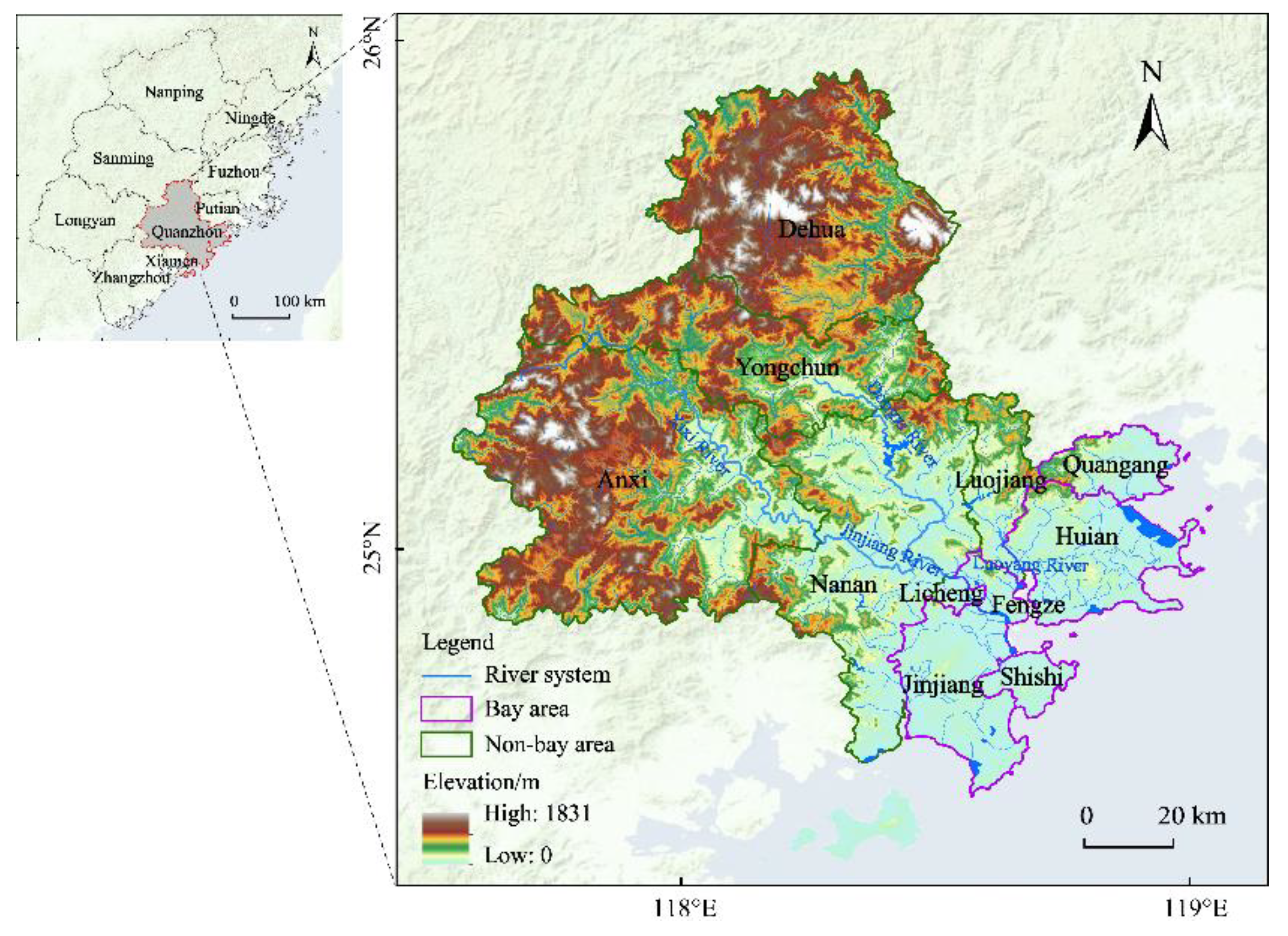
2.1. Study Area

The municipality of Quanzhou is located at a low latitude in the southeast coastal area of China, and it features a subtropical, maritime monsoon climate with relatively moderate weather. It is one of the three central cities in the Fujian Province to the south of Fuzhou City (the capital of Fujian Province), north of Xiamen Special Zone, and west of Taiwan island (Figure 1). The city borders the sea and rolling mountains, and it covers a land area of 11,015 km² (including Jinmen not involved in this study). There are 34 rivers with watershed areas greater than 100 km² originating here, with a total length of 1549 km. The Jinjiang River and Luoyang River converge into the sea at Quanzhou Bay. It has a twisting coastline of 541 km and active deep-sea ports with abundant coastal resources and higher environmental carrying capacities.

2.2. Data Sources

In this paper, five types of data sets were applied: land use classification maps, digital elevation model (DEM) data, demographic data, transportation data, and socioeconomic data as listed in

Table 1. Summary of the data sets used in this study.

Dataset Types	Source	Time Period
Land use and cover (1 km × 1 km)	the Resource and Environmental Science Data Center of the Chinese Academy of Sciences (http://www.resdc.cn, accessed on 5 March 2021)	2005; 2010; 2015
Digital elevation model (30 m × 30 m)	Geospatial Data Cloud (https://www.gscloud.cn, accessed on 5 March 2021)	-
Transportation data	91 Satellite Image Assistant	-
Socioeconomic data	Quanzhou Statistics Yearbook (http://www.quanzhou.gov.cn, accessed on 12 March 2021)	2006; 2011; 2016
Demographic data	Quanzhou Land Use Overall Planning (2006–2020)	-

.

2.3. Methods

2.3.1. Evaluation Model of Supply Capacity of Ecosystem Services

Ecosystem services are mainly classified into provisioning services, regulation services, cultural services, and supporting services. As supporting services are the basis and premise of the first three types of services, and they are not directly related to human well-being, this paper only evaluated provisioning services, regulation services, and cultural services [37]. On the basis of previous foundations, a quantitative model was developed to measure the supply capacity of ecosystem services using land use classification maps. The following formula reflects the spatialization of supply capacity of ecosystem services on a 1 km grid:

$$E_s={{\displaystyle \sum }}_{u=1}^n{{\displaystyle \sum }}_{i=1}^6\frac{S_{iu}}{S}\left(k_{ia}+k_{ib}+k_{ic}\right) \left(i=1,2,3,4,5,6\right)$$

(1)

where $E_s$ is the dimensionless evaluation index of the supply capacity of ecosystem services, and $i$ represents six types of land use including arable land, forest, grassland, water area, construction land, and unused land. $a$, $b$, and $c$ represent provisioning services, regulation services, and cultural services, respectively. $S_{iu}$ is the area of land use $i$ in cell $u$, and $S$ is the total area of the grid cells in the study site. $k_{ia}$ is the correlation intensity among provisioning services and various land use types; analogously, $k_{ib}$ is the intensity among regulating services and land use types, and $k_{ic}$ is associated with cultural services. The specific values are shown in

Table 2. The intensity and K value of ecosystem services supply of various land use types.

Land Use	K Value Assignment Based on the Subdivision of Various Land Use Types
	Land Cover (Subdivision)	Provisioning Services		Regulating Services		Cultural Services
		Intensity	K	Intensity	K	Intensity	K
Arable land	Non-irrigated land	21	20	5	5	1	0
	Irrigated land	18		5		1
Forest	Broadleaf forest	21	21	39	39	10	10
	Mixed forest	21		39		10
Grassland	Natural grassland	30	30	8	8	3	3
Water area	Channel	12	12	10	8	10	10
	Water area	12		7		9
Construction land	Mean value of urban land use	2	2	0	0	0	0
Unused land	Unused land	0	0	2	2	0	0

.

The arable land in Quanzhou is mainly paddy field, and irrigated land accounts for most of the basic farmland. The research used the average value of irrigated land and non-irrigated land to represent the K value of arable land. According to the land use data and statistical data, forestry resources are concentrated in northwestern Quanzhou, where forest is the largest land cover type. The K value of forestland depends on the average value of broadleaf forest and mixed forest, which provide two main kinds of local resources. Grasslands serve the functions of providing food for livestock and enhancing soil and water conservation. Given the underdevelopment of animal husbandry in the study area, natural grassland was selected as a reference for the grassland K value. There are many rivers and streams in Quanzhou, but lakes occupy only a small area. Therefore, the correlation coefficient was based on the mean value of the two water types. For construction land, the K value was based on the average value of 11 secondary types in the land use classification system. Unused land in Quanzhou only occupies a small space, while saline land occupies most of the space. Hence, unused land was assigned the value that was assigned to saline land in the relevant literature.

2.3.2. Evaluation Model of Consumption Demand of Ecosystem Services

Consulting the study by Burkhard and Kroll [4], this paper constructed another evaluation model to quantify the consumption demand of ecosystem services:

$$E_d={{\displaystyle \sum }}_{u=1}^n{{\displaystyle \sum }}_{i=1}^6\frac{S_{iu}}{S}\left(d_{ia}+d_{ib}+d_{ic}\right) \left(i=1,2,3,4,5,6\right)$$

(2)

where $E_d$ is the dimensionless evaluation index of the consumption demand of ecosystem services and $d_{ia}$, $d_{ib}$, and $d_{ic}$ are the correlation coefficients among the three kinds of ecosystem services and various land use types. The other parameters are explained in Equation (1). The assignment principles are identical to those of the supply capacity of ecosystem services (

Table 3. The intensity and K value of ecosystem services demand of various land use types.

Land Use	K Value Assignment Based on Subdivision of Various Land Use Types
	Land Cover (Subdivision)	Provisioning Services		Regulating Services		Cultural Services
		Intensity	K	Intensity	K	Intensity	K
Arable land	Non-irrigated land	3	6	15	20	0	0
	Irrigated land	9		25		0
Forest	Broadleaf forest	3	3	0	0	0	0
	Mixed forest	3		0		0
Grassland	Natural grassland	9	9	8		0	0
Water area	Channel	1	1	0	8	0	0
	Water area	1		0	0	0
Construction land	Mean value of urban land use	43	43	32	32	6	6
Unused land	Unused land	0	0	0	32	0	0

).

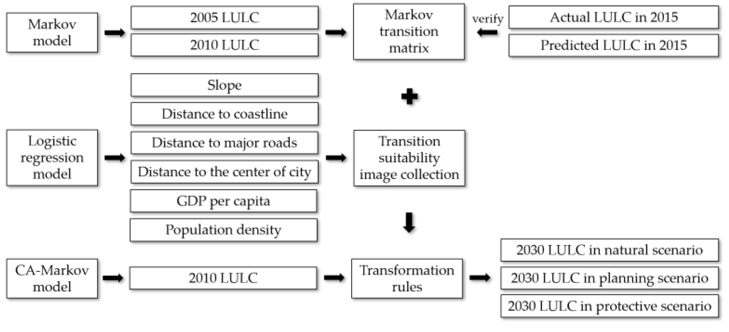
2.3.3. Markov–Logistic–CA Model

The Markov model is a trend prediction model used to calculate the land use area transfer matrix, which assumes that the future state can be simulated by the previous state [38]. The Markov process is the prediction of land use structural change based on the land use transfer probability [39]. As in Equation (3):

$$N_{\left(t+1\right)}=R_{ij}\times N_{\left(t\right)}$$

(3)

where $N_{\left(t+1\right)}$ is the state of the land use type at time $t+1$ and $N_{\left(t\right)}$ is the state at time $t$.

Then, the driving factors influencing land use change are analyzed using a binary logistic regression model. At present, the allocation model primarily based on land use suitability evaluation has become the basis of the spatial prediction model [40]. The logistic regression algorithm can select a series of explanatory variables (topography, population density, distance from cities, accessibility) to describe the potential possibility of land use change [41,42]. The standard linear regression model is as follows [43]:

$$Logit\left(B_i\right)=\ln \left(\frac{B_i}{1-B_i}\right)={\beta }_0+{\beta }_1{x}_1+{\beta }_2{x}_2+{\beta }_3{x}_3+\cdots +{\beta }_n{x}_n$$

(4)

where $B_i$ is the probability of a particular land use type $i$ that appears in each grid, and $X$ is an independent variable representing various driving forces. The model can be regarded as an empirical approach to deriving the probability of one land use type converting to another in the next period of time. It also demonstrates the relationship between observations and dependent variables. The study used the ROC curve as an indicator to verify the factors’ significance.

Finally, we ran the CA model to simulate the spatiotemporal dynamic evolution of land use types. The cellular automata model can map the quantitative predictions of the Markov model in space, emphasizing the neighborhood interactions among the cells scattered in the regular grid [44]. Space and time are discrete, while the interaction is local. The state of each cell at the next moment is jointly determined by itself and its surrounding neighbor cells [45], following the transition rule corrected by the logistic regression model for simultaneous updates [46]. The state of the system moves forward in discrete time steps [47]. It can be expressed as follows [48]:

$$D_{\left(t+1\right)}=f\left(D_{\left(t\right)},G\right)$$

(5)

where $D$ is the set of all possible states of the cells, and $f$ is a transition function defining the rules of the state changing from $t$ to $t+1$. $G$ represents the neighbourhood of the cells as input values for the function $f$.

2.4. Data Pre-Proceeding

As a basic for research, logistic regression was used to filter the main drivers of land use change, including slope, distance to coastline, GDP per capita, distance to the center of city, distance to major roads, and population density. Then combined the suitability images of spatial distribution probability with Markov transition matrix, we defined the transformation rules for CA (Figure 2). To confirm the effectiveness of the model, the simulated LULC map in 2015 was compared with the actual map. The areas of various land use types in Quanzhou from 2005 to 2015 are listed in

Table 4. Land use changes in Quanzhou during 2005–2015.

Year	Area (km2)
	Arable Land	Forest	Grassland	Water	Construction Land	Unused Land
2005	2599	5489	1659	126	972	8
2010	2526	5480	1640	125	1075	9
2015	2475	5482	1634	124	1131	8

. The kappa coefficient was 0.9197, indicating that the model was reliable as a predictive tool [38,45]. With respect to Quanzhou’s planning strategy and ecological security protection, the study set three kinds of scenarios, including natural scenario, planning scenario, and protection scenario. Using the LULC map in 2010, the CA–Markov model, available in the IDRISI 7.0 software, was able to predict the LULC maps in 2030 and corresponding areas of various land use types (

Table 5. Land use area in Quanzhou in 2030 under different scenarios.

Scenario	Area (km2)
	Arable Land	Forest	Grassland	Water	Construction Land	Unused Land
Current situation in 2015	2475	5482	1634	124	1131	8
Natural scenario in 2030	2266	5040	1480	145	1895	28
Planning scenario in 2030	2366	5300	1500	141	1519	28
Protective scenario in 2030	2386	5340	1520	165	1415	28

) in different scenarios.

3. Results

3.1. Evaluation Results of Supply and Demand of Ecosystem Services

Applying Equations (1) and (2), we quantized the supply capacity and consumption demand of ecosystem services. Supply-demand balance can reflect regional ecological security to a certain extent.

Table 6. The change in supply and demand of ecosystem services in Quanzhou (dimensionless).

Ecosystem Services		2005	2010	2015
Provisioning services	Supply capacity	182,752	180,974	179,999
	Consumption demand	92,485	96,307	98,729
	Supply-demand difference	90,267	84,667	81,720
Regulating services	Supply capacity	241,488	240,611	240,269
	Consumption demand	47,630	50,422	51,892
	Supply-demand difference	193,858	190,189	188,377
Cultural services	Supply capacity	63,726	63,496	63,457
	Consumption demand	20,076	20,645	20,975
	Supply-demand difference	43,650	42,851	42,482
Total	Supply capacity	487,966	485,081	483,725
	Consumption demand	92,485	96,307	98,729
	Supply-demand difference	90,267	84,667	81,720

shows how these factors changed over time. During 2005–2015, the supply capacity was greater than the consumption demand in any year, meaning that the supply could meet the demand of consumption and the supply-demand structure of ecosystem services in Quanzhou was acceptable. The total supply capacity and difference decreased, while the overall demand increased by 6.8% in 10 years. Specifically, the supply capacity of all three services continuously decreased. Among the three types of services, regulating services had the largest gap, which illustrated that they were the most sustainable. In addition, the difference between the supply and demand of the provisioning services was the lowest, and it showed the fastest decline. Although in a relatively safe range, they were the most prone to imbalance.

According to the supply and demand of the ecosystem services valuation model, the types of land use providing services are mainly arable land, forestland, and grassland, while the demand for ecosystem services comes primarily from human residential areas. This reminds us to protect ecological land properly so as to curb this trend that might affect ecological security in Quanzhou.

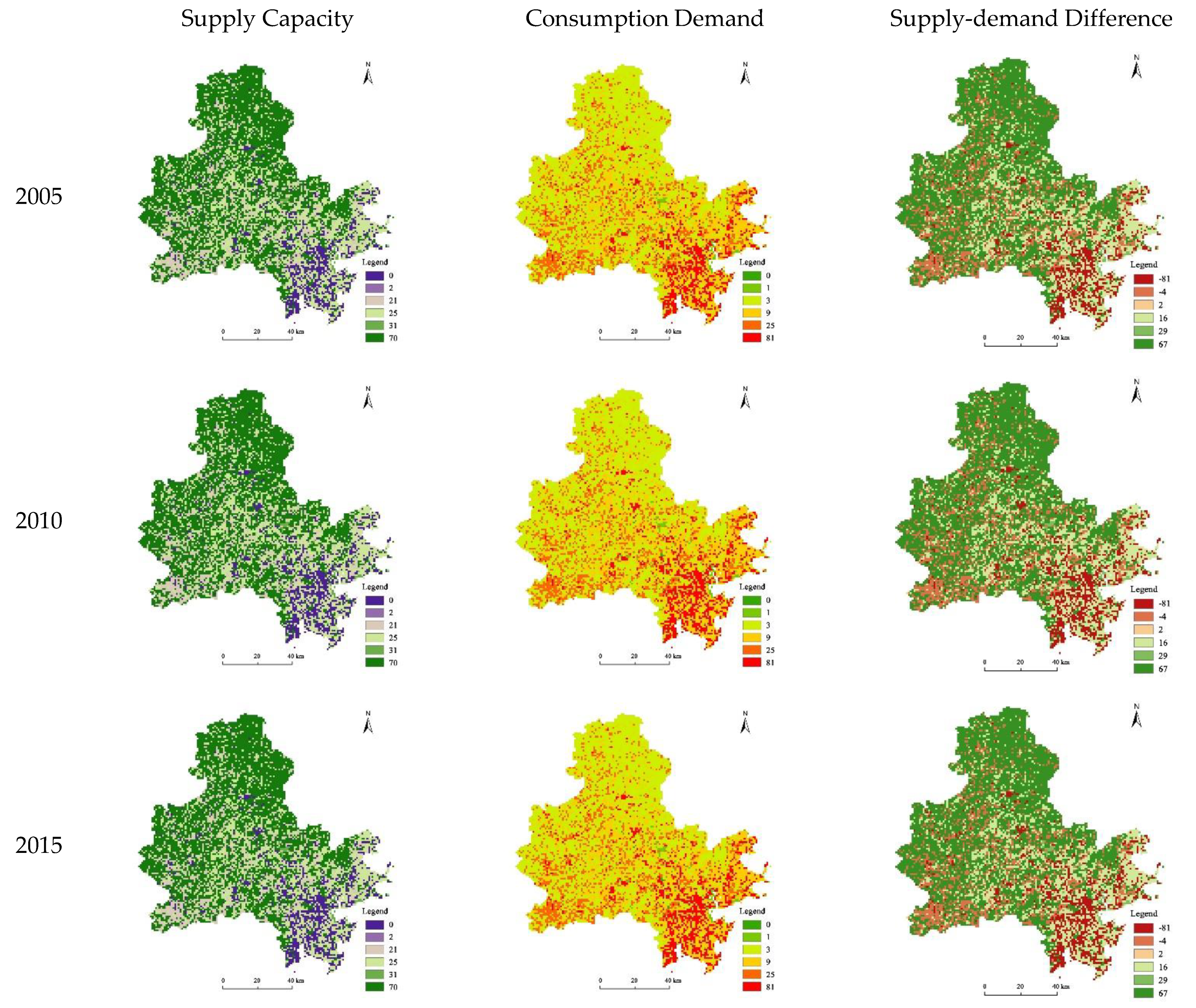
3.2. Spatial Pattern of Supply and Demand of Ecosystem Services

We used ArcGIS to realize the spatialization of supply capacity and consumption demand in Quanzhou based on a 1 km × 1 km raster layer of land use from 2005 to 2015. The spatial heterogeneity in different years enabled the identification of supply and demand hotspots of ecosystem services as well as the change features.

Figure 3 demonstrates that there was apparent spatial regularity in the supply and demand status that was caused by factors of geographical conditions and regional economic development differences. The supply capacity of ecosystem services showed a decreasing trend from northwest to southeast. Concurrently, the high-value areas were mainly concentrated in the upper reaches of the river basin, including Anxi, Yongchun and Dehua, mountainous counties just north of Quanzhou. Anxi had the highest forest coverage in Quanzhou. Extensive forests and grasslands provided higher ecosystem services, while less construction land reduced the demand in this region. The low-value areas were distributed in downstream watersheds, such as Jinjiang, Shishi, Nanan, and a part of the main urban area.

The consumption demand was opposite to the supply capacity in the spatial distribution law. High-value areas of consumption demand were mostly found in the southeast bay area, where arable land and construction land occupy most of the space and ecological land is minimal. Drastic changes in land use and continuous reductions in ecological land were attributed to this area’s in situ urbanization with regional characteristics, further resulting in a low supply capacity of ecosystem services. The spatial distribution law of the supply-demand difference was consistent with that of the consumption demand. The superposition of less supply and more demand made this law more obvious, and even the gap in some areas was negative.

Table 7. Contrast of supply and demand of ecosystem services between bay area and non-nay area in 2015 (dimensionless).

Region	Supply Capacity	Consumption Demand	Supply-Demand Difference
Bay area	24.07	31.05	−6.98
Non-bay area	48.79	12.60	36.19

illustrates the contrast of the mean supply and demand of ecosystem services between bay areas and non-bay areas in 2015. We found that the supply capacity in the bay area was only approximately half of that in the non-bay area, while the consume demand was 2.5 times higher in the bay area. The bay area exerted significantly more pressure on supply and demand. In terms of the difference, the negative value in the bay area indicated that the supply and demand of ecosystem services was in a state of imbalance, which calls for sustainable development and signals a threat to ecological security.

3.3. Analysis of Supply and Demand of Ecosystem Services in Different Scenarios

Currently, we have summarized the reasons for the imbalance between supply and demand of ecosystem services in Quanzhou. Predicting the situation in the future will help us deeply examine the spatial pattern to explore how factors influence the balance of supply and demand of ecosystem services. Meanwhile, scenario simulations can be used to study alterations in supply and demand under different scenarios to provide a decision-making reference for regional ecological security protection. This paper predicted LULC changes in 2030 according to trends in the dynamics, and then the supply and demand of ecosystem services were assessed.

The extent of land area change was limited in the planning scenario in accordance with the planning objectives. The conversion of forest land, arable land, and grassland to construction land was reduced by 10% in the protective scenario and the conversion of water bodies to construction land is prohibited. Overall,

Table 8. Contrast of ecosystem services supply and demand in 2030 under different scenarios (dimensionless).

Ecosystem Services		Current Situation in 2015	Natural Scenario in 2030	Planning Scenario in 2030	Protective Scenario in 2030
Provisioning services	Supply capacity	179,999	201,090	208,390	210,270
	Consumption demand	98,729	123,666	108,886	105,026
	Supply-demand difference	81,270	77,424	99,504	105,254
Regulating services	Supply capacity	240,269	220,946	231,746	233,726
	Consumption demand	51,892	117,800	107,800	105,160
	Supply-demand difference	188,377	103,146	123,946	128,566
Cultural services	Supply capacity	63,457	56,290	58,950	59,610
	Consumption demand	20,975	23,210	21,090	20,650
	Supply-demand difference	42,482	33,080	37,860	38,960
Total	Supply capacity	483,725	478,326	499,086	503,606
	Consumption demand	171,146	264,676	237,776	230,836
	Supply-demand difference	312,579	213,650	261,310	272,770

displays that the total supply capacity in the natural scenario (478,326) was lower than that in 2015 (483,725), while an upwards trend was shown in the planning scenario and protection scenario. The result demonstrated that the protection and planning of ecological security can improve the supply capacity of ecosystem services. The total consumption demand increased by a large margin, and the rising range was highest in the natural scenario, which explained why the human demand for ecological services was increasing. In 2030, the supply-demand difference declined in the three simulated scenarios. The magnitude of the drop was greatest in the natural scenario, followed by the planning scenario and the protection scenario. In terms of provisioning services, the supply and demand in 2030 were higher than those in 2015, and the difference decreased only in the natural scenario. For regulating services and cultural services, there were declines in supply capacity and differences and increases in demand in the future. Among them, the gap in the natural scenario was the lowest.

4. Discussion

4.1. The Contradiction between Supply and Demand under Rapid Urbanization

The unique resources of bay areas and their complex “human–environment” ecosystems are the basis for their development. The natural and open characteristics of bay areas have been proven to be of special value in the long-term urban development process [49]. The gathering of labor, capital, technology, and other production factors brings significant momentum to urbanization. It increases the demand for limited natural resources in coastal areas. At the same time, rural areas are faced with the challenges of rural–urban migration and its effect on land transfer [50]. The sharp conflicts in land use may affect frequent material exchange, energy flow, and other ecological processes within the watershed, resulting in a mismatch between the supply and demand of ecosystem services [51], especially at small and medium scales. Research has been carried out on the value assessment and functional spatial optimization of ecosystem services in bay areas under rapid urbanization [52,53,54], but few studies have explored the ecosystem response to human activities from the perspective of supply and demand of ecosystem services.

In general, the supply and demand of ecosystem services in Quanzhou are in surplus. The provisioning services, regulating services, and cultural services provided by ecosystems are able to meet local consumption demand. However, the tension between supply and demand is reflected not only in the total amount but also in the types, values, and diversity demands in the spatial and temporal distribution of ecosystem services that regions can provide [15]. During the period from 2005 to 2015, along with the changes in land use and the transformation of ecological land to construction land, the difference between the supply and demand of all three ecosystem services showed a decreasing trend with the most obvious decrease in provisioning services. This warns us of the potential ecological security risks in the future supply and demand pattern of ecosystem services in Quanzhou. This is similar to the evolutionary characteristics of ecosystem services supply and demand in developing countries resulting from massive land development and utilization due to the fact of urbanization demands [55]. In terms of spatial patterns, the bay area of Quanzhou corresponds to the offshore area of the lower reaches of the basin, while the non-bay area corresponds to the inland area of the upper reaches. The supply capacity of ecosystem services is spatially characterized as low offshore and high inland, while the consumption demand shows the opposite pattern, creating a state of imbalance between supply and demand in the bay area as confirmed by Huang et al. [56]. Some studies have indicated that in bay area basins, the value of ecosystem services tends to be higher in the inland hinterland than in the lower reaches offshore [57]. The areas where significant changes occur on a temporal scale are usually concentrated at the sea-land boundary [58]. This illustrates that the economic activities of stakeholders have become the main factors in the supply and demand patterns of ecosystem services [59]. The spatial relationship between service provision areas and beneficiary areas and the contradiction between supply and demand are challenges to be faced in the urbanization process.

4.2. Policy Implications for Land Use Management

The mismatch between the supply and demand of ecosystem services is multidimensional, not only in terms of temporal and spatial variability but also in trade-offs between costs and benefits for stakeholders [60,61]. The negative impacts of a supply-demand mismatch often have a time-lag effect. Sustainable management of natural resources depends on scientific and reasonable prediction of the spatial distributions and changing trends of the supply and demand of ecosystem services [62]. The scenario simulation method provides technical support for dynamic monitoring and early warning of supply and demand trends as well as a reference for policy on weighing ecological construction and urbanization expansion.

Among the three scenarios simulated for 2030, the difference between the supply and demand of ecosystem services in Quanzhou under the natural scenario decreased the most compared to those in 2015. Although the difference also decreased in the protective scenario and planning scenario under development target constraints and land use control, the decline was much smaller than that in the natural scenario, indicating that the imbalance between the supply and demand of ecosystem services can be reduced through the optimal allocation of land use [63]. Managers could exercise strict control over the amount of green space and blue space to maintain the supply of ecosystem services [64], but that may not necessarily achieve the policy goal of minimizing the imbalance between supply and demand [65]. What we need to recognize is that the complexity of natural-economic ecological systems poses enormous challenges in trade-offs and synergies between ecosystem services and human well-being, different types of services and multiple stakeholders.

As key regions in the spatial extent of the blue economy, the utilization and management of bays is a priority for coastal development [66]. Watersheds with different dominant land use patterns may respond differently to supply and demand of ecosystem services. Typically, ecosystem services tend to be provided from the upstream supply areas of the watershed to the downstream demand areas along hydrologic flow paths. Potential intervention points can be determined by referring to the simulation results of the supply and demand relationship of ecosystem services in Quanzhou. According to the objectives of different decision-making priorities in the region, we should comprehensively consider the ecological and economic benefits, measures what needs to be adjusted and the aspects of well-being that need to be improved. It is vital to facilitate hierarchical management. The core focus in the southeast bay area is limiting the direction and scale of expansion of construction land instead of the crude land use pattern that grabs important ecological land such as forests and water bodies. While in the northwest mountainous counties with higher capacity to supply ecosystem services of Quanzhou, compensation protection zones and buffer zones should be established to develop an ecological economy and improve the effective supply and value realization of ecological services from the inland hinterland to the bay area. At the same time, the government needs to play a leading role in promoting the interregional flow of supply and demand of ecosystem services on a larger scale. It is helpful to implement rational resource development, ecological compensation formulations, and bay protection decisions in a planned and organized manner.

4.3. Limitations and Future Research Direction

This study used an advanced matrix to measure the supply and demand of ecosystem services with reference to the results of a study by German researchers that semi-quantitatively reflected on the differences in supply and demand among different LULC types. The choice of regions and the research focus of the experts may have affected the evaluation of the results to a certain extent [67,68]. Meanwhile, data without dimensions have not been able to provide a basis for horizontal comparison between different ecosystem services. Considering the influence of land classification methods and data accuracy, the matrix method based on LULC was not sufficient to fully reflect the internal heterogeneity of supply and demand of the same land use type. Undeniably, the method still has a certain applicability in general, especially in areas where data are scarce for quickly identifying key spatial points and providing useful information for environmental management [69,70,71].

In addition, this paper only identified and predicted the spatial differences and contradictions between the supply and demand of ecosystem services at the local scale within a city. However, the supply and demand areas of ecosystem services do not completely coincide geographically [72]. In fact, only a few ecosystem services are consumed locally in the supply areas, while most ecosystem services flow between the supply and benefit areas and are influenced by a variety of human and natural factors, such as water provisioning and cultural services [73], which are remotely coupled. Ecosystem service flows can dynamically couple ecosystem service supply with human demand and clarify the impacts of changes in ecosystem services on human well-being [74]. In the future, the current research system should be improved by combining ecosystem service flows to analyze the structural match between supply and demand in terms of the flow rate, outflow, flow direction, and accessibility of different types of ecosystem services. The delivery pathways and flow processes of ecosystem services from supply areas to beneficiary areas could be considered, which would reveal the driving mechanisms and causal links between supply and demand of ecosystem services. Furthermore, the model’s predictive capability should be enhanced to provide future scenarios with high confidence levels to explore regional-scale cooperation from the perspective of multiple stakeholders.

5. Conclusions

Using Quanzhou as a case study, this study estimated the supply capacity and consumption demand of three important ecosystem services, provisioning services, regulating services, and cultural services from 2005 to 2015 with an accounting model based on multisource data. On this basis, the paper discussed the spatiotemporal dynamic evolution of the supply and demand of ecosystem services under different scenarios in 2030. We found that, on the whole, the supply capacity of ecosystem services could meet the demand of consumption and the supply-demand balance was relatively healthy in Quanzhou. However, the supply-demand difference of the three services showed a downwards trend (most dramatically in provisioning services). The high-value areas of supply capacity were concentrated in the upper reaches of the river basin, while the high-value areas of consumption demand were mostly found in the southeast bay area. The superposition of less supply and more demand led to an imbalance between supply and demand in the bay area as well as a threat to the ecological security. Among the three simulated scenarios in 2030, the supply-demand difference decreased to a certain extent compared with that in 2015. The magnitude of the drop was greatest in the natural scenario followed by the planning scenario and the protection scenario. We expect these findings to provide a decision-making reference for ecological security and natural resource management in bay areas and to promote the exploration of territorial spatial planning based on ecological bottom lines.

References

1. Al-Mohannadi, A.S.; Furlan, R. The practice of city planning and design in the gulf region: The case of Abu Dhabi, Doha and Manama. Archnet-IJAR 2018, 12, 126–145. [Google Scholar] [CrossRef]
2. Niu, B.; Ge, D.; Yan, R.; Ma, Y.; Sun, D.; Lu, M.; Lu, Y. The evolution of the interactive relationship between urbanization and land-use transition: A case study of the yangtze river delta. Land 2021, 10, 804. [Google Scholar] [CrossRef]
3. Boyd, J.; Banzhaf, S. What are ecosystem services? The need for standardized environmental accounting units. Ecol. Econ. 2007, 63, 616–626. [Google Scholar] [CrossRef] [Green Version]
4. Burkhard, B.; Kroll, F.; Nedkov, S.; Mueller, F. Mapping ecosystem service supply, demand and budgets. Ecol. Indic. 2012, 21, 17–29. [Google Scholar] [CrossRef]
5. Zhang, Z.; Peng, J.; Xu, Z.; Wang, X.; Meersmans, J. Ecosystem services supply and demand response to urbanization: A case study of the Pearl River Delta, China. Ecosyst. Serv. 2021, 49, 101274. [Google Scholar] [CrossRef]
6. Wei, H.; Liu, H.; Xu, Z.; Ren, J.; Lu, N.; Fan, W.; Zhang, P.; Dong, X. Linking ecosystem services supply, social demand and human well-being in a typical mountain-oasis-desert area, Xinjiang, China. Ecosyst. Serv. 2018, 31, 44–57. [Google Scholar] [CrossRef]
7. Schirpke, U.; Candiago, S.; Vigl, L.E.; Jager, H.; Labadini, A.; Marsoner, T.; Meisch, C.; Tasser, E.; Tappeiner, U. Integrating supply, flow and demand to enhance the understanding of interactions among multiple ecosystem services. Sci. Total Environ. 2019, 651, 928–941. [Google Scholar] [CrossRef]
8. Zander, K.K.; Straton, A. An economic assessment of the value of tropical river ecosystem services: Heterogeneous preferences among Aboriginal and non-Aboriginal Australians. Ecol. Econ. 2010, 69, 2417–2426. [Google Scholar] [CrossRef]
9. Bai, Y.; Wang, M.; Li, H.; Huang, S.; Alatalo Juha, M. Ecosystem service supply and demand: Theory and management application. Acta Ecol. Sin. 2017, 37, 5846–5852. [Google Scholar]
10. Syrbe, R.-U.; Walz, U. Spatial indicators for the assessment of ecosystem services: Providing, benefiting and connecting areas and landscape metrics. Ecol. Indic. 2012, 21, 80–88. [Google Scholar] [CrossRef]
11. Yan, Y.; Zhu, J.; Wu, G.; Zhan, Y. Review and prospective applications of demand, supply, and consumption of ecosystem services. Acta Ecol. Sin. 2017, 37, 2489–2496. [Google Scholar]
12. Ayanu, Y.Z.; Conrad, C.; Nauss, T.; Wegmann, M.; Koellner, T. Quantifying and mapping ecosystem services supplies and demands: A review of remote sensing applications. Environ. Sci. Technol. 2012, 46, 8529–8541. [Google Scholar] [CrossRef] [PubMed]
13. Burkhard, B.; Kandziora, M.; Hou, Y.; Müller, F. Ecosystem service potentials, flows and demands—Concepts for spatial localisation, indication and quantification. Landsc. Online 2014, 34, 1–32. [Google Scholar] [CrossRef]
14. Wolff, S.; Schulp, C.J.E.; Verburg, P.H. Mapping ecosystem services demand: A review of current research and future perspectives. Ecol. Indic. 2015, 55, 159–171. [Google Scholar] [CrossRef]
15. Ma, L.; Liu, H.; Peng, J.; Wu, J. A review of ecosystem services supply and demand. Acta Geogr. Sin. 2017, 72, 1277–1289. [Google Scholar]
16. Semmens, D.J.; Diffendorfer, J.E.; Lopez-Hoffman, L.; Shapiro, C.D. Accounting for the ecosystem services of migratory species: Quantifying migration support and spatial subsidies. Ecol. Econ. 2011, 70, 2236–2242. [Google Scholar] [CrossRef]
17. Fisher, B.; Turner, R.K.; Morling, P. Defining and classifying ecosystem services for decision making. Ecol. Econ. 2009, 68, 643–653. [Google Scholar] [CrossRef] [Green Version]
18. Pataki, D.E.; Carreiro, M.M.; Cherrier, J.; Grulke, N.E.; Jennings, V.; Pincetl, S.; Pouyat, R.V.; Whitlow, T.H.; Zipperer, W.C. Coupling biogeochemical cycles in urban environments: Ecosystem services, green solutions, and misconceptions. Front. Ecol. Environ. 2011, 9, 27–36. [Google Scholar] [CrossRef]
19. Zhao, W.; Liu, Y.; Feng, Q.; Wang, Y.; Yang, S. Ecosystem services for coupled human and environment systems. Prog. Geogr. 2018, 37, 139–151. [Google Scholar]
20. Fu, B.; Forsius, M. Ecosystem services modeling in contrasting landscapes. Landsc. Ecol. 2015, 30, 375–379. [Google Scholar] [CrossRef] [Green Version]
21. Peng, J.; Tian, L.; Zhang, Z.; Zhao, Y.; Green, S.M.; Quine, T.A.; Liu, H.; Meersmans, J. Distinguishing the impacts of land use and climate change on ecosystem services in a karst landscape in China. Ecosyst. Serv. 2020, 46, 101199. [Google Scholar] [CrossRef]
22. Wang, J.; Sui, L.; Yang, X.; Wang, Z.; Ge, D.; Kang, J.; Yang, F.; Liu, Y.; Liu, B. Economic globalization impacts on the ecological environment of inland developing countries: A case study of laos from the perspective of the land use/cover change. Sustainability 2019, 11, 3940. [Google Scholar] [CrossRef] [Green Version]
23. Sturck, J.; Poortinga, A.; Verburg, P.H. Mapping ecosystem services: The supply and demand of flood regulation services in Europe. Ecol. Indic. 2014, 38, 198–211. [Google Scholar] [CrossRef]
24. Larondelle, N.; Lauf, S. Balancing demand and supply of multiple urban ecosystem services on different spatial scales. Ecosyst. Serv. 2016, 22, 18–31. [Google Scholar] [CrossRef]
25. Wang, L.; Zheng, H.; Wen, Z.; Liu, L.; Robinson, B.E.; Li, R.; Li, C.; Kong, L. Ecosystem service synergies/trade-offs informing the supply-demand match of ecosystem services: Framework and application. Ecosyst. Serv. 2019, 37, 100939. [Google Scholar] [CrossRef]
26. Burkhard, B.; Kroll, F.; Müller, F.; Windhorst, W. Landscapes‘ capacities to provide ecosystem services—A concept for land-cover based assessments. Landsc. Online 2009, 15, 1–12. [Google Scholar] [CrossRef]
27. Pena, L.; Casado-Arzuaga, I.; Onaindia, M. Mapping recreation supply and demand using an ecological and a social evaluation approach. Ecosyst. Serv. 2015, 13, 108–118. [Google Scholar] [CrossRef]
28. Li, J.; Jiang, H.; Bai, Y.; Alatalo, J.M.; Li, X.; Jiang, H.; Liu, G.; Xu, J. Indicators for spatial-temporal comparisons of ecosystem service status between regions: A case study of the Taihu River Basin, China. Ecol. Indic. 2016, 60, 1008–1016. [Google Scholar] [CrossRef]
29. Cai, W.; Gibbs, D.; Zhang, L.; Ferrier, G.; Cai, Y. Identifying hotspots and management of critical ecosystem services in rapidly urbanizing Yangtze River Delta Region, China. J. Environ. Manag. 2017, 191, 258–267. [Google Scholar] [CrossRef]
30. Gonzalez-Garcia, A.; Palomo, I.; Gonzalez, J.A.; Lopez, C.A.; Montes, C. Quantifying spatial supply-demand mismatches in ecosystem services provides insights for land-use planning. Land Use Policy 2020, 94, 104493. [Google Scholar] [CrossRef]
31. Palacios-Agundez, I.; Onaindia, M.; Potschin, M.; Tratalos, J.A.; Madariaga, I.; Haines-Young, R. Relevance for decision making of spatially explicit, participatory scenarios for ecosystem services in an area of a high current demand. Environ. Sci. Policy. 2015, 54, 199–209. [Google Scholar] [CrossRef]
32. Sauter, I.; Kienast, F.; Bolliger, J.; Winter, B.; Pazur, R. Changes in demand and supply of ecosystem services under scenarios of future land use in Vorarlberg, Austria. J. Mt. Sci. 2019, 16, 2793–2809. [Google Scholar] [CrossRef]
33. Jager, H.; Peratoner, G.; Tappeiner, U.; Tasser, E. Grassland biomass balance in the European Alps: Current and future ecosystem service perspectives. Ecosyst. Serv. 2020, 45, 101163. [Google Scholar] [CrossRef]
34. Li, S.; Zhang, C.; Liu, J.; Zhu, W.; Ma, C.; Wang, J. The tradeoffs and synergies of ecosystem services: Research progress, development trend, and themes of geography. Geogr. Res. 2013, 32, 1379–1390. [Google Scholar]
35. Brunner, S.H.; Huber, R.; Gret-Regamey, A. A backcasting approach for matching regional ecosystem services supply and demand. Environ. Model. Softw. 2016, 75, 439–458. [Google Scholar] [CrossRef] [Green Version]
36. Meisch, C.; Schirpke, U.; Huber, L.; Rudisser, J.; Tappeiner, U. Assessing freshwater provision and consumption in the alpine space applying the ecosystem service concept. Sustainability 2019, 11, 1131. [Google Scholar] [CrossRef] [Green Version]
37. Ou, W.; Wang, H.; Tao, Y. A land cover-based assessment of ecosystem services supply and demand dynamics in the Yangtze River Delta region. Acta Ecol. Sin. 2018, 38, 6337–6347. [Google Scholar]
38. Subedi, P.; Subedi, K.; Thapa, B. Application of a hybrid cellular automaton—Markov (CA-Markov) model in land-use change prediction: A case study of Saddle Creek Drainage Basin, Florida. Appl. Ecol. Environ. Sci. 2013, 1, 126–132. [Google Scholar] [CrossRef] [Green Version]
39. Mohamed, A.; Worku, H. Simulating urban land use and cover dynamics using cellular automata and Markov chain approach in Addis Ababa and the surrounding. Urban Clim. 2020, 31, 100545. [Google Scholar] [CrossRef]
40. Saxena, A.; Jat, M.K. Land suitability and urban growth modeling: Development of SLEUTH-Suitability. Comput. Environ. Urban. Syst. 2020, 81, 101475. [Google Scholar] [CrossRef]
41. Wang, H.; Kong, X.; Zhang, B. The simulation of LUCC based on Logistic-CA-Markov model in Qilian Mountain area, China. Sci. Cold Arid Reg. 2016, 8, 350–358. [Google Scholar]
42. Han, Y.; Jia, H. Simulating the spatial dynamics of urban growth with an integrated modeling approach: A case study of Foshan, China. Ecol. Model. 2017, 353, 107–116. [Google Scholar] [CrossRef]
43. Munshi, T.; Zuidgeest, M.; Brussel, M.; van Maarseveen, M. Logistic regression and cellular automata-based modelling of retail, commercial and residential development in the city of Ahmedabad, India. Cities 2014, 39, 68–86. [Google Scholar] [CrossRef]
44. Liao, J.; Tang, L.; Wang, C.; Xu, T. Measuring and calibrating extended neighborhood effect of urban cellular automata model based on particle swarm optimization. Prog. Geogr. 2014, 33, 1624–1633. [Google Scholar]
45. Parsa, V.A.; Yavari, A.; Nejadi, A. Spatio-temporal analysis of land use/land cover pattern changes in Arasbaran Biosphere Reserve: Iran. Model. Earth Syst. Environ. 2016, 2, 1–13. [Google Scholar] [CrossRef]
46. Liu, H.; Zhang, Z.; Shui, W.; Wang, Q.; Yang, Y. Urban growth boundary delimitation of resource-exhausted cities: A case study of Huaibei City. J. Nat. Resour. 2017, 32, 391–405. [Google Scholar]
47. Arsanjani, J.J.; Helbich, M.; Kainz, W.; Boloorani, A.D. Integration of logistic regression, Markov chain and cellular automata models to simulate urban expansion. Int. J. Appl. Earth Obs. Geoinf. 2013, 21, 265–275. [Google Scholar] [CrossRef]
48. Gong, X.; Bian, J.; Wang, Y.; Jia, Z.; Wan, H. Evaluating and predicting the effects of land use changes on water quality using SWAT and CA-Markov models. Water Resour. Manag. 2019, 33, 4923–4938. [Google Scholar] [CrossRef]
49. Llope, M. The ecosystem approach in the Gulf of Cadiz. A perspective from the southernmost European Atlantic regional sea. ICES J. Mar. Sci. 2017, 74, 382–390. [Google Scholar] [CrossRef]
50. Xu, D.; Yong, Z.; Deng, X.; Zhuang, L.; Qing, C. Rural-urban migration and its effect on land transfer in rural China. Land 2020, 9, 81. [Google Scholar] [CrossRef] [Green Version]
51. Li, Y.; Feng, Y.; Guo, X.; Peng, F. Changes in coastal city ecosystem service values based on land use A case study of Yingkou, China. Land Use Policy 2017, 65, 287–293. [Google Scholar] [CrossRef]
52. Du, Y.; Shui, W.; Sun, X.-R.; Yang, H.-F.; Zheng, J.-Y. Scenario simulation of ecosystem service trade-offs in bay cities: A case study in Quanzhou, Fujian Province, China. J. Appl. Ecol. 2019, 30, 4293–4302. [Google Scholar]
53. Aguilera, M.A.; Tapia, J.; Gallardo, C.; Nunez, P.; Varas-Belemmi, K. Loss of coastal ecosystem spatial connectivity and services by urbanization: Natural-to-urban integration for bay management. J. Environ. Manag. 2020, 276, 111297. [Google Scholar] [CrossRef] [PubMed]
54. Fang, Y.; Zhai, T.; Zhao, X.; Chen, K.; Guo, B.; Wang, J. Study on the comprehensive improvement of ecosystem services in a China’s bay city for spatial optimization. Water 2021, 13, 2072. [Google Scholar] [CrossRef]
55. Dofrtzbach, D.; Blainski, É.; Farias, M.; Pereira, A.; Pereira, M.; Paz-González, A. Landscape dynamic analysis of use and land cover of Camboriu and Balneario Camboriu, SC. Cad. Pru. Geogr. 2015, 37, 5–26. [Google Scholar]
56. Huang, Z.; Wang, F.; Cao, W. Dynamic analysis of an ecological security pattern relying on the relationship between ecosystem service supply and demand: A case study on the Xiamen- Zhangzhou-Quanzhou city cluster. Acta Ecol. Sin. 2018, 38, 4327–4340. [Google Scholar]
57. Liu, Y.; Li, J.; Yuan, Q.; Shi, X.; Pu, R.; He, G. A comparative study on the changes of ecosystem services values in the bay basin between China and the USA: A case study on Xiangshangang Bay basin, Zhejiang and Tampa Bay basin, Florida. Geogr. Res. 2019, 38, 357–368. [Google Scholar]
58. Liu, R.; Xu, H.; Li, J.; Pu, R.; Sun, C.; Cao, L.; Jiang, Y.; Tian, P.; Wang, L.; Gong, H. Ecosystem service valuation of bays in East China Sea and its response to sea reclamation activities. J. Geogr. Sci. 2020, 30, 1095–1116. [Google Scholar] [CrossRef]
59. Chaplin-Kramer, R.; Sharp, R.P.; Weill, C.; Bennett, E.M.; Pascual, U.; Arkema, K.K.; Brauman, K.A.; Bryant, B.P.; Guerry, A.D.; Haddad, N.M.; et al. Global modeling of nature’s contributions to people. Science 2019, 366, 255–258. [Google Scholar] [CrossRef]
60. Wei, H.; Fan, W.; Wang, X.; Lu, N.; Dong, X.; Zhao, Y.; Ya, X.; Zhao, Y. Integrating supply and social demand in ecosystem services assessment: A review. Ecosyst. Serv. 2017, 25, 15–27. [Google Scholar] [CrossRef]
61. Wang, W.; Wu, T.; Li, Y.; Zheng, H.; Ouyang, Z. Matching ecosystem services supply and demand through land use optimization: A study of the Guangdong-Hong Kong-Macao megacity. Int. J. Env. Res. Public Health. 2021, 18, 2324. [Google Scholar] [CrossRef]
62. Maes, J.; Egoh, B.; Willemen, L.; Liquete, C.; Vihervaara, P.; Schaegner, J.P.; Grizzetti, B.; Drakou, E.G.; La Notte, A.; Zulian, G.; et al. Mapping ecosystem services for policy support and decision making in the European Union. Ecosyst. Serv. 2012, 1, 31–39. [Google Scholar] [CrossRef]
63. Strauch, M.; Cord, A.F.; Paetzold, C.; Lautenbach, S.; Kaim, A.; Schweitzer, C.; Seppelt, R.; Volk, M. Constraints in multi-objective optimization of land use allocation—Repair or penalize? Environ. Model. Softw. 2019, 118, 241–251. [Google Scholar] [CrossRef]
64. Chen, J.; Jiang, B.; Bai, Y.; Xu, X.; Alatalo, J.M. Quantifying ecosystem services supply and demand shortfalls and mismatches for management optimisation. Sci. Total Environ. 2019, 650, 1426–1439. [Google Scholar] [CrossRef] [PubMed]
65. Ruckelshaus, M.; McKenzie, E.; Tallis, H.; Guerry, A.; Daily, G.; Kareiva, P.; Polasky, S.; Ricketts, T.; Bhagabati, N.; Wood, S.A.; et al. Notes from the field: Lessons learned from using ecosystem service approaches to inform real-world decisions. Ecol. Econ. 2015, 115, 11–21. [Google Scholar] [CrossRef] [Green Version]
66. Komar, P.D. Shoreline evolution and management of Hawke’s bay, New Zealand: Tectonics, coastal processes, and human impacts. J. Coastal Res. 2010, 26, 143–156. [Google Scholar] [CrossRef]
67. Hou, Y.; Burkhard, B.; Mueller, F. Uncertainties in landscape analysis and ecosystem service assessment. J. Environ. Manag. 2013, 127, 117–131. [Google Scholar] [CrossRef]
68. Kaiser, G.; Burkhard, B.; Roemer, H.; Sangkaew, S.; Graterol, R.; Haitook, T.; Sterr, H.; Sakuna-Schwartz, D. Mapping tsunami impacts on land cover and related ecosystem service supply in Phang Nga, Thailand. Nat. Hazards Earth Syst. 2013, 13, 3095–3111. [Google Scholar] [CrossRef] [Green Version]
69. Jacobs, S.; Burkhard, B.; van Daele, T.; Staes, J.; Schneiders, A. ‘The Matrix Reloaded’: A review of expert knowledge use for mapping ecosystem services. Ecol. Model. 2015, 295, 21–30. [Google Scholar] [CrossRef]
70. Paudyal, K.; Baral, H.; Burkhard, B.; Bhandari, S.P.; Keenan, R.J. Participatory assessment and mapping of ecosystem services in a data-poor region: Case study of community-managed forests in central Nepal. Ecosyst. Serv. 2015, 13, 81–92. [Google Scholar] [CrossRef]
71. Uthes, S.; Matzdorf, B. Budgeting for government-financed PES: Does ecosystem service demand equal ecosystem service supply? Ecosyst. Serv. 2016, 17, 255–264. [Google Scholar] [CrossRef]
72. Brauman, K.A.; Daily, G.C.; Duarte, T.K.; Mooney, H.A. The nature and value of ecosystem services: An overview highlighting hydrologic services. Annu. Rev. Environ. Resour. 2007, 32, 67–98. [Google Scholar] [CrossRef]
73. Koellner, T.; Bonn, A.; Arnhold, S.; Bagstad, K.J.; Fridman, D.; Guerra, C.A.; Kastner, T.; Kissinger, M.; Kleemann, J.; Kuhlicke, C.; et al. Guidance for assessing interregional ecosystem service flows. Ecol. Indic. 2019, 105, 92–106. [Google Scholar] [CrossRef]
74. Liu, H.M.; Fan, Y.L.; Ding, S.Y. Research progress of ecosystem service flow. Chin. J. Appl. Ecol. 2016, 27, 2161–2171. [Google Scholar]
Figure 1. Location of the study area.
Land 11 00022 g001
Figure 2. Workflow of Markov-Logistic-CA model.
Land 11 00022 g002
Figure 3. Spatial–temporal pattern of supply capacity, consumption demand, and supply-demand difference of ecosystem services in Quanzhou.
Land 11 00022 g003