Article

Ecological Corridor Construction Based on Least-Cost Modeling Using Visible Infrared Imaging Radiometer Suite (VIIRS) Nighttime Light Data and Normalized Difference Vegetation Index

1
College of Public Administration, South-Central University for Nationalities, Wuhan 430074, China
2
School of Resource and Environmental Science, Wuhan University, Wuhan 430079, China
3
College of Urban and Environmental Sciences, Central China Normal University, Wuhan 430079, China
*
Author to whom correspondence should be addressed.
Land 2021, 10(8), 782; https://doi.org/10.3390/land10080782
Submission received: 23 June 2021 / Revised: 22 July 2021 / Accepted: 22 July 2021 / Published: 26 July 2021
(This article belongs to the Section Landscape Ecology)

Abstract

:
Anthropic pressure is one of the main drivers of landscape change and biodiversity loss. Artificial nighttime light, which can affect species behavior, is an important human-induced threat to biodiversity, but it is often ignored in ecological connectivity research. To mitigate the adverse impacts of artificial lighting on biodiversity, this study integrates artificial nighttime light in landscape ecology and analyzes the influence of artificial nighttime light on landscape connectivity. A quantitative approach integrating nighttime light brightness from a Visible Infrared Imaging Radiometer Suite (VIIRS) with a normalized difference vegetation index (NDVI) from a Moderate-resolution Imaging Spectroradiometer (MODIS) is proposed to estimate the matrix resistance, which can identify the sensitive areas that are disrupted by nighttime light. It was found that the nightscape in the study area is significantly disrupted by nighttime light and the matrix resistance in the center of the study area significantly increases. Compared to the least-cost routes from the NDVI, the “dark” least-cost ecological corridors constructed using our approach apparently change in both location and distance. The corridors moved to the outer suburbs and rural areas, and the maximum increase in distance of the least-cost paths was 37.94%. Due to less disturbance from human activity and the maintenance of a pristine nightscape, “dark” ecological corridors can reduce the adverse effects of night lights and contribute to biodiversity. However, natural habitats have been greatly affected by nighttime light with the increase in global illumination, and it is essential that we improve public awareness of light pollution and formulate light-reduction policies and legislation.

1. Introduction

Over the last several centuries, increasing anthropic pressures and land-use changes have fragmented natural habitats and caused rapid declines in biodiversity [1]. Conservation scientists believe that large and well-connected patches can contribute to higher biodiversity [2,3]. Hence, it is necessary to construct ecological network on large-scale land areas [4,5]. Ecological networks mainly consist of habitat patches and ecological corridors [6]. To construct effective ecological networks, it is important to consider the size of the habitat patches, which needs to be big enough to support populations of the focal species [7,8]. In addition, ecological corridors need to be constructed between different habitat patches to encourage the unimpeded movement of various species and the flow of natural processes [9]. The ecological network is of great significance in the protection of biodiversity in fragmented ecosystems, and is highly valued by planners and land managers, being widely constructed all over the world [10].
The construction of ecological networks can conserve biodiversity, largely because they restore and maintain ecological connectivity [11]. Ecological connectivity can be divided into structural connectivity and functional connectivity [12]. Structural connectivity only considers the continuity of habitat patches in space, while functional connectivity focuses on the movements of organisms between habitat patches [3]. As it may be difficult to track enough individuals of some species, tracking umbrella species can identify connectivity areas for a set of species [13]. Theoretically, the construction of ecological corridors can be conducive to the migration of organisms among fragmented habitat patches and can alleviate the negative effects of habitat fragmentation; therefore, the construction of ecological corridors has been regarded as one of the main means of regional biodiversity conservation [3]. There is a growing number of quantitative approaches to modeling ecological corridors, such as circuit theory, individual-based modeling, and least-cost modeling [14,15,16]. Least-cost modeling is based on graph theory and incorporates the effects of the intervening matrix. A resistance surface is needed in the model which indicates the difficulty of species’ movements. Matrix resistance can be estimated by experts based on empirical knowledge of the behavior of the focal species and environmental variables, such as land use, land cover, elevation, hydrology, and slope [17,18,19,20,21,22]. Matrix resistance can also be estimated based on naturalness which assumes that as naturalness increases, resistance to species movements decreases [23,24]. Baldwin et al. calculated matrix resistance based on the human footprint [25]. The normalized difference vegetation index (NDVI), which is computed from satellite imagery and linked to vegetation cover and animal distribution and abundance, can provide the information needed to estimate matrix resistance [26,27].
In most studies, however, differences in the landscapes between daytime and nighttime conditions are ignored. The outdoor nighttime light environment has been transformed by the gradual spread of urbanization and electrification [28,29]. Direct light from electrical lighting, reflected light from the surrounding areas, and sky glow scattered in the atmosphere create a highly polluted environment [30,31]. Approximately 30% of all vertebrates and more than 60% of all invertebrates around the world are nocturnal [32]. Artificial nighttime light has disrupted the natural cycles of light and dark; altered natural light regimes spatially, temporally, and spectrally; affected the foraging and reproduction patterns of organisms; changed behavior and movement patterns, especially in light-repelled species; and formed barriers of continuously lit linear pathways, such as roads [30,33,34,35,36]. Nocturnal satellite images of the Earth provide a convenient way to monitor spatial variability and temporal changes in night lights; thus, this technique has been widely used to examine the ecological impacts of artificial light pollution. Historically, research on remote sensing nighttime light has primarily used Defense Meteorological Satellite Program (DMSP) imagery. The Visible Infrared Imaging Radiometer Suite (VIIRS) sensor that was launched in 2011, which offers higher spatial resolution and improved capabilities for quantifying nighttime brightness, has shown better results than the DMSP sensor [37].
Most research has focused on the detrimental consequences of artificial nighttime light on a species level. However, there has been a lack of attention paid to artificial nighttime light on a landscape level. With the increase in global illumination, natural habitats have been greatly affected by nighttime light. Some vegetated areas which are considered to provide high matrix permeability and have a high conservation value have been polluted by nighttime light. As nighttime light may damage the spatial behavior of nocturnal species [38], moving through these areas will come at a greater cost to them. In addition, there will be an increase in the matrix resistance and a decrease in connectivity in these vegetated areas.
In this study, we considered the influence of artificial nighttime light on landscape ecology and proposed a new method to estimate matrix resistance based on the normalized difference vegetation index (NDVI) and VIIRS data to construct “dark” ecological corridors. We analyzed the detrimental consequences of artificial nighttime light on the matrix in a fast-growing urbanized landscape in Wuhan in Central China. Matrix resistance was calibrated using our own methods, and, for contrast, we calculated matrix resistance from NDVI data alone. Next, we used least-cost modeling to build ecological corridors and compared the differences between day and night. Our study provides another perspective on how lights could affect species movement at night, and can help to optimize landscape planning and mitigate the adverse consequences of artificial lights in macroecology.

2. Materials and Methods
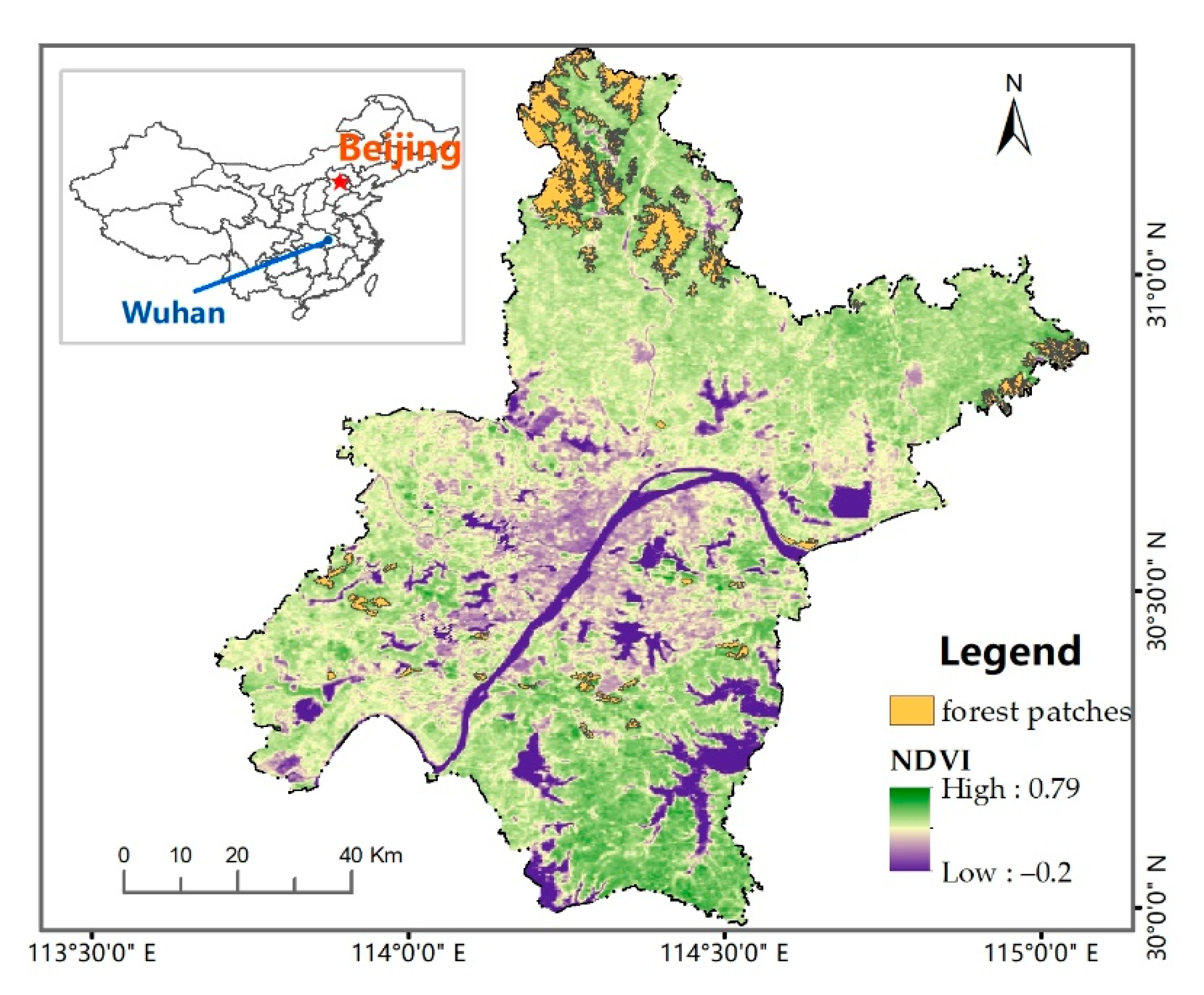
2.1. Study Area

To study the impacts of artificial nighttime light on landscape connectivity, Wuhan, a fast-growing city, was selected as the study site. It is situated in the middle reaches of the Yangtze River region in Central China, between the parallels 29°58′ N and 31°22′ N and the meridians 113°41′ E and 115°05′ E (Figure 1). The total area of Wuhan is 8594 km2, of which 22.88% is under forest cover. Wuhan has a subtropical monsoon climate, and the forest cover is mainly dominated by evergreen broad-leaved forests and deciduous broad-leaved forests. The main nocturnal species in the study area include Bufo gargarizans, Fejervarya multistriata, Myotis chinensis, Rhinolophus sinicus, and some Strigiformes species, such as the Collared Owl and Red Horned Owl. As a result of rapid urbanization in recent decades, the natural habitats have shrunk and become fragmented, and anthropization is one of the main risk factors that threatens the landscape connectivity and biodiversity [39].
For connectivity analysis, source patches need to be selected according to patch area, landscape suitability, and accessibility [40]. In the study area, the source patches contained 56 forest patches with the minimum ecological threshold set at 100 ha [41,42]. Forest patches were scattered in this landscape with complex shapes and edges due to human influence on the land surface. The average area was 714.09 ha, ranging from 106.19 to 12,137.48 ha, and their total area covered 4.58% of the whole study area. The vector map of forest patches was created from land surveys by the Wuhan Land Resources and Planning Bureau.

2.2. Data Sources and Processing

The Visible Infrared Imaging Radiometer Suite (VIIRS) aboard the Suomi-NPP satellite was launched on 28 October 2011, collecting high-quality nighttime images in the Day/Night Band (DNB). The 2015 VIIRS Nighttime Lights Annual Composite (from 20150101 to 20151231) from a version 1 suite of average radiance composite images was downloaded from https://eogdata.mines.edu/products/vnl/ (accessed on 15 October 2020) in 2020. The products were produced in 15 arc-second geographic grids and distributed in radiance values with units in nW/cm2/sr [43]. The “vcm-orm” image for this study was cloud-free, and fires and other ephemeral lights were filtered out. The VIIRS DNB image was resampled at 250 m to match the spatial resolution of the MODIS NDVI datasets described below.
NDVI, calculated from reflectance in the red and near-infrared wavebands, is one of the most commonly used vegetation indices for characterizing vegetation conditions and variations. The 2015 16-day NDVI datasets (observations from 20150101 to 20151231) were downloaded from the MODIS (Moderate-Resolution Imaging Spectroradiometer) MOD13Q1 V.6 dataset at a spatial resolution of 250 m in 2020 [44]. Images were checked for possible contamination using the MOD13Q1 quality layer [45]. Next, the average NDVI value for 2015 was calculated from the 16-day NDVI images.

2.3. Analysis Methods

2.3.1. Matrix Resistance from the Nighttime Light Adjusted Vegetation Index (NAVI)

NDVI, the most commonly used vegetation index, is strongly related to biological diversity and can easily provide an approximation of habitat suitability and matrix resistance for species [46]. Since its invention, electrical lighting has been brought to nearly every corner of the planet and has dramatically transformed the outdoor nighttime light environment and nightscape. Nighttime light represents the human influence on ecosystems during the night and has influenced the movements of nocturnal species [29].
In this study, we propose the nighttime light adjusted vegetation index (NAVI), which considers the influence of nighttime light on habitat suitability and integrates nighttime light into NDVI to study the suitability of the matrix for organisms during the night [47]. It is defined in the following expression:
NAVI = ( 1 NTL ) × NDVI
where NDVI is calculated as NDVI = (NIR − RED)/(NIR + RED), where NIR and RED are the near-infrared and red wavebands from MODIS. NDVI values range between −1 and +1. Denser vegetation cover always means higher NDVI values. For the MODIS NDVI, negative values usually represent water and glaciers. Nighttime light was from the VIIRS DNB, which was normalized by the brightest pixel in the scene (i.e., dividing the radiance value of each pixel by the maximum value in the scene). In order to eliminate the influence of extremely high values in urban areas, the average value of the most prosperous area of the study area was calculated as the maximum brightness value. Subsequently, the nighttime light brightness value for all pixels were divided by the maximum value. For those with a normalized nighttime light value higher than 1, the value was converted to 1, constraining the values of normalized nighttime light (NTL) between 0 and 1.
According to the NAVI, denser and darker areas mean a lower cost for organisms to move through them. Thus, the reciprocal of the NAVI(RNAVI) is taken as a measure for matrix resistance:
RNAVI = 1 NDVI × ( 1 NTL )
For contrast, we also estimated matrix resistance with NDVI only. The resistance values were calculated by the reciprocal of NDVI(RNDVI):
RNDVI = 1 NDVI
The resistance value was set to 1000 when the NDVI or NAVI value was less than 0.001.

2.3.2. Least-Cost Path

The least-cost path analysis is based on graph theory and calculates effective distances and optimal pathways based on the minimum cumulative resistance (MCR, which is the cumulative distance from a certain landscape unit with the resistance value linked to the ecological source) between habitat patches [19]. The cost distance function is an algorithm of the grid data, moving from the center to the periphery of the eight units. As shown in Equation (4), the cumulative cost that any Ni moves to four vertically adjacent units Ni+1 is half of the total cost coefficient moving from Ni to Ni+1. As shown in Equation (5), the cumulative cost that any Ni moves to four diagonally adjacent units Ni+1 is the product of half of the total cost coefficient moving from Ni to Ni+1 and the square root of 2:
N i + 1 = N i + r i + r i + 1 2
N i + 1 = N i + 2 × ( r i + r i + 1 ) 2
where Ni and ri represent the cumulative cost and the cost coefficient of unit i, respectively; Ni+1 and ri+1 represent the cumulative cost and the cost coefficient of moving to unit i + 1, respectively.
To identify and map least-cost paths, a resistance layer should be created. The resistance value of each cell is based on how the matrix facilitates or impedes movement of the species. In our study, the resistance value of each cell was measured by RNLVI or RNDVI. The least-cost paths were constructed after calculating the minimum accumulated cost surface. Cost was calculated between the edges of habitat patches. We did not set up a threshold distance and connected all the adjacent forest patches identified using the ArcGIS allocation function. These steps were undertaken with ArcGIS and Linkage Mapper [16].

2.3.3. Analysis of Nightscape Change and Comparison of Connectivity Results

With direct light from electrical lighting, reflected light from the surrounding areas, and sky glow scattered in the atmosphere, large areas were illuminated. To analyze how nighttime light was distributed in our study area and how nighttime light influenced the sources and matrix, we calculated the scope and intensity of nighttime light. We calculated a statistic of nighttime light brightness every 2 km from the brightest cell in the central city as well as values of NDVI for contrast, and then calculated the average brightness value of the source patches.
By the same method, we calculated a statistic of NDVI and NAVI values every 2 km from the brightest cell in the central city to determine the nightscape change when considering nighttime light. Next, we compared the resistance surface from NDVI and that from NAVI. The final connection results were shown as paths between forest patches. To quantitatively compare connections during the day and night, the differences between the two distances were calculated with the following equation:
f ( x ) = ( y i - x i ) x i
where x is the least-cost distance from NDVI, and y is the least-cost distance from NAVI.

3. Results

3.1. Analysis of Nightscape Change

In our study area, the brightest cell appeared in the central business district in Hankou, the value of which was 162.13 nW/cm2/sr. We detected a significant decrease from the center to the margin by calculating the average values every 2 km from the brightest cell (Figure 2a). The average brightness value of core areas was 56.47 nW/cm2/sr, and it rapidly decreased to approximately 10 nW/cm2/sr at 20 km from the central city. Next, continuous dark areas appeared after approximately 40 km, with average brightness values of less than 1 nW/cm2/sr (Figure 2b). Most of the forest patches were far from the central area, the average brightness value of which was 0.373 nW/cm2/sr, showing little influence from nighttime light. However, the NDVI showed a converse pattern compared to the distribution of nighttime light, indicating a slow linear increase from built-up areas to the rural and natural areas with a slope of 0.0078 (R2 = 0.9433).
We created an overlay analysis of the images from the NDVI and VIIRS DNB to determine how nighttime light penetrated the matrix. The NDVI and VIIRS DNB brightness values were continuous field datasets, and to better show the results, the values of both images were grouped into six categories (Table 1). The matrix with higher NDVI values and lower brightness values was more suitable for organism movement. Of the total area, 35.08% had a VIIRS DNB brightness value of more than 1 nW/cm2/sr, and 11.94% had a VIIRS DNB brightness value of more than 10 nW/cm2/sr. Of the total areas, 82.64% had an NDVI value of more than 0.3, in which 29.61% had a VIIRS DNB brightness value of more than 1 nW/cm2/sr.
We compared the average value of the NDVI and NAVI every 2 km from the center (Figure 2b). The original NDVI values showed a smooth increase from the center to the margin. Due to the influence of nighttime light, the NAVI values showed apparent variation, especially within 40 km. The NAVI values in the central area became extremely low due to the presence of built-up districts with the highest intensities of artificial light all night. Further from the city, the difference narrowed, and NAVI values were almost the same as those of NDVI. Two frequency histograms are shown in Figure 3 to compare the statistical distributions of the values of the NDVI and NAVI. The grid numbers of the NAVI experienced a significant increase of approximately 0 due to the extremely high brightness values in the central city, and then a smooth increase within 0.25 and a decrease within 0.36.

3.2. Comparison of Ecological Network Results

The reciprocal of NDVI or NAVI was used to estimate the matrix resistance. Two resistance surfaces were built. To better show the difference between the two resistance surfaces, we subtracted RNDVI from RNAVI. The result is shown in Figure 4. Since nighttime light primarily influenced the central part of the study area, it was apparent that values in the center were brighter than on the periphery. More energy and resources were required for organisms to cross the central area.
The ecological networks in our study area were visualized in two ways: as least-cost paths or least-cost corridors between forest patches. The least-cost paths were the routes along which the least resistance was accumulated (lines with different colors in Figure 5). Actual ecological corridors usually require a certain width and have a different cost compared with the least-cost paths. The least-cost corridors are the bands with a certain width and have the minimum difference in cost compared with the least-cost paths. The least-cost paths were classified into five groups according to their distances by natural breaks (Figure 5a,b). In general, distances in marginal areas were shorter than in the central area owing to better matrix qualities and less human influence in both maps. Distances calculated from RNAVI were longer than those from RNDVI.
The differences between two distances were calculated with Equation (6). Most routes in the north experienced a change of less than 1% due to the minimal influence of nighttime light. However, some routes experienced a large change in both location and distances. We located the routes that changed location and changed more than 5% in distance, arranged them in order from large to small variation, and renumbered them, where 1 represented the largest change at 37.94% (Figure 6). These routes were distributed in the center of the study area, moving to the outer suburbs and rural areas when nighttime light was considered. Although there was usually a high greening rate in the suburbs, nighttime light had a great impact on the nightscape of the suburbs and the matrix quality deteriorated with the expansion of the city, the extension of urban roads, and the penetration of urban lifestyle, changing the location and distances of these routes.
Notes: Cost difference means the minimum difference in the cost of passing a certain cell compared with the least-cost paths.

4. Discussion

It is important to consider human influence on ecological connectivity and biodiversity conservation. Human influence is one of the main drivers of landscape change and loss of biodiversity [48,49]. Nighttime light pollution caused by humans has influenced the physiological and behavioral pattern of organisms, and thus threatened biodiversity, but it has been persistently ignored in macroecology and ecological connectivity research [50,51]. We found that the matrix in our study area was significantly disrupted by nighttime light. The brightness value of 11.94% of the study area was more than 10 nW/cm2/sr, of which the NDVI value of 51.6% was more than 0.3. Nighttime light caused the matrix to become more complex and fragmented and changed the landscape during night, which affected the simulation results of ecological corridors. Ecological corridors are fundamental elements in ecological networks due to their key role in maintaining or restoring ecological connectivity, and in the conservation of biodiversity. In order to facilitate the movement of as many species as possible, ecological corridors need to have high vegetation coverage and as little human disturbance as possible [3]. If nighttime light is not contemplated in the construction of the corridors, some vegetated areas with high light pollution may be considered as ecological corridors of high conservation value. In consequence, some nocturnal species such as bats, owls, and fireflies may suffer negative impacts. For example, it has been found that light pollution may damage the spatial behavior of bats and cause a reduction in their survival and reproductive capacity [52]. Therefore, if light pollution is not considered in the planning and protection of ecological corridors, the absence of effective protection for nocturnal species may lead to cascade effects which may result in a deterioration in ecosystem function and biodiversity protection on a landscape scale [53]. Hence, it is important in practice to consider the detrimental consequences of artificial nighttime light on the matrix when constructing ecological corridors.
Our analysis is based on graph theory and uses the least-cost path to model structural connectivity, in which NDVI and VIIRS DNB data are integrated to estimate matrix resistance. The NDVI, a widely used vegetation index in ecological and geographical research, can indicate the extent of vegetation cover and matrix quality. VIIRS data, which display the extent of night lights, is an ideal proxy to map the land surface that is influenced, or may be influenced, by human activity. In many development zones, lights illuminate the matrix along the newly built roads and construction sites before they are deeply disrupted. Hence, ecological corridors that are constructed using our approach can contribute more to landscape connectivity and biodiversity due to less disturbance from human activity and the maintenance of the pristine nightscape. Additionally, both NDVI and VIIRS DNB data can be easily accessed from remote sensing, and will facilitate the dynamic planning, monitoring, and protection of ecological corridors. However, it is notable that there are seasonal changes in NDVI and VIIRS nighttime brightness. The seasonal changes of the NDVI in the study area, which are highly correlated with the seasonal growth of vegetation, are significant because the forest cover is mainly dominated by evergreen broad-leaved forests and deciduous broad-leaved forests. As shown in Figure 7, the highest NDVI value appears in August (summer in the lunar calendar) and the lowest NDVI value appears in February (winter in the lunar calendar). The seasonal changes in VIIRS nighttime brightness have been found to be positively correlated with seasonal changes in snow cover and albedo, and negatively correlated with seasonal changes in vegetation cover [54]. Moreover, human activity seasonality could also impact the seasonal changes in nighttime brightness [55]. As shown in Figure 7, the lowest values of nighttime brightness appear in February and March, which may be due to the Spring Festival holidays. In our study, yearly static images were used to construct ecological corridors on a large scale. However, if constructing ecological corridors for specific species on a small scale, seasonal changes may need to be considered.
Our results offer a preliminary basis for understanding how nighttime light influences ecological connectivity. Due to the adverse effects of nighttime light on nocturnal species, moving through a matrix polluted by nighttime light comes at a higher cost, meaning that the matrix permeability and connectivity decrease. Comparing the connectivity results using two distances, routes in the central area apparently changed in both location and distance. The routes moved to the outer suburbs and rural areas, and the maximum increase in distance of the least-cost paths reached 37.94%. Though ecological corridors constructed using our approach can reduce the adverse effects of night lights, it is not enough for the protection of ecosystems and biodiversity. With the increase in global illumination, natural habitats have been greatly affected by nighttime light, and the risk of losing many light-sensitive species also increases [56]. However, light pollution is different from other forms of pollution (e.g., air pollution), and it is relatively easy to reverse. Measures such as reducing the intensity of lighting, changing the spectral composition of lighting, and limiting the duration of lighting could be implemented to effectively reduce light pollution [57]. Light reduction policies and legislation may be effective. However, due to a poor understanding of light pollution, improving public awareness and participation is also very significant [58].
However, the application of satellite-based nighttime light data has some limitations. Typical nighttime light images, such as DMSP and VIIRS, have disadvantages such as low resolution and blooming effect, which make it difficult for fine planning and management of ecological corridors on a small scale [59]. Further development of the light detection sensor and data processing algorithms are still of great importance, with the possibility of providing more data products with a higher resolution and a higher detection ability. Moreover, the DNB band of VIIRS, used as a proxy for nighttime light in this study, only represents light intensity. Indeed, light intensity is just one of the properties of light that can affect species behavior, with the spectral composition of light and the duration of lighting also being important [60]. Hence, an integration of nighttime light data and other data from both satellite-based and ground-based observation would merit more efforts in the future.

5. Conclusions

To mitigate the adverse consequences of artificial lights on biodiversity, this study integrated artificial nighttime light in landscape ecology and analyzed the influence of artificial nighttime light on landscape connectivity. A quantitative approach integrating data of nighttime light from VIIRS DNB with NDVI from MODIS was proposed to estimate matrix resistance, which can identify the sensitive areas that are disrupted by nighttime light. It was found that matrix resistance in the center of the study area significantly increased and the nightscape and ecological connectivity in our study area was significantly disrupted by nighttime light. Compared to the least-cost routes from the NDVI, the “dark” ecological corridors constructed using our approach in the center of study area apparently changed in both location and distance. The corridors moved to the outer suburbs and rural areas, and the maximum increase in distance of the least-cost paths was 37.94%. Due to less disturbance from human activity and the maintenance of a pristine nightscape, “dark” ecological corridors can reduce the adverse effects of night lights and contribute to biodiversity. However, with an increase in global illumination, natural habitats have been greatly affected by nighttime light, and it is essential that we improve public awareness of light pollution and formulate light-reduction policies and legislation.

Author Contributions

Conceptualization, J.H. and Y.L.; data curation, J.H.; formal analysis, Y.L. and J.F.; funding acquisition, J.F.; investigation, Y.L.; methodology, J.H.; project administration, Y.L.; resources, J.F.; software, J.F.; supervision, J.F.; validation, J.F.; visualization, J.F.; writing—original draft, J.H.; writing—review & editing, Y.L. and J.F. All authors have read and agreed to the published version of the manuscript.

Funding

This research was funded by the National Natural Science Foundation of China, grant number 42077441.

Acknowledgments

The authors are very grateful for the constructive comments and suggestions from the editors and anonymous reviewers.

Conflicts of Interest

The authors declare no conflict of interest.

References

  1. Butchart, S.H.M. Global Biodiversity: Indicators of Recent Declines. Science 2010, 328, 1164–1168. [Google Scholar] [CrossRef] [PubMed]
  2. Borregaard, M.K.; Matthews, T.J.; Whittaker, R.J. The general dynamic model: Towards a unified theory of island biogeography? Glob. Ecol. Biogeogr. 2016, 25, 805–816. [Google Scholar] [CrossRef]
  3. Hilty, J.; Worboys, G.L.; Keeley, A.; Woodley, S.; Lausche, B.J.; Locke, H.; Carr, M.; Pulsford, I.; Pittock, J.; White, J.W.; et al. Guidelines for Conserving Connectivity through Ecological Networks and Corridors; Groves, C., Ed.; International Union for Conservation of Nature: Gland, Switzerland, 2020. [Google Scholar] [CrossRef]
  4. Bunn, A.G.; Urban, D.L.; Keitt, T.H. Landscape connectivity: A conservation application of graph theory. J. Environ. Manag. 2000, 59, 265–278. [Google Scholar] [CrossRef] [Green Version]
  5. Avon, C.; Bergès, L. Prioritization of habitat patches for landscape connectivity conservation differs between least-cost and resistance distances. Landsc. Ecol. 2016, 31, 1551–1565. [Google Scholar] [CrossRef] [Green Version]
  6. Zhou, D.; Song, W. Identifying Ecological Corridors and Networks in Mountainous Areas. Int. J. Environ. Res. Public Health 2021, 18, 4797. [Google Scholar] [CrossRef] [PubMed]
  7. Green, A.L.; Fernandes, L.; Almany, G.; Abesamis, R.; McLeod, E.; Alino, P.M.; White, A.T.; Salm, R.; Tanzer, J.; Pressey, R.L. Designing Marine Reserves for Fisheries Management, Biodiversity Conservation, and Climate Change Adaptation. Coast. Manag. 2014, 42, 143–159. [Google Scholar] [CrossRef]
  8. Shi, F.N.; Liu, S.L.; An, Y.; Sun, Y.X.; Zhao, S.; Liu, Y.X.; Li, M.Q. Spatio-Temporal Dynamics of Landscape Connectivity and Ecological Network Construction in Long Yangxia Basin at the Upper Yellow River. Land 2020, 9, 265. [Google Scholar] [CrossRef]
  9. Jongman, R.H.G. Nature Conservation Planning in Europe—Developing Ecological Networks. Landsc. Urban Plan. 1995, 32, 169–183. [Google Scholar] [CrossRef]
  10. Sorvig, K. Ecological networks and greenways: Concept, design, implementation. Landsc. Archit. 2005, 95, 137. [Google Scholar]
  11. Tabor, G.; Bankova-Todorova, M.; Correa Ayram, C.; Garcia, L.; Kapos, V.; Olds, A.; Stupariu, I. Ecological Connectivity: A Bridge to Preserving Biodiversity; United Nations Environment Programme: Nairobi, Kenya, 2019; pp. 24–37. [Google Scholar]
  12. Tischendorf, L.; Fahrig, L. On the usage and measurement of landscape connectivity. Oikos 2000, 90, 7–19. [Google Scholar] [CrossRef] [Green Version]
  13. Mukherjee, T.; Sharma, L.K.; Kumar, V.; Sharief, A.; Dutta, R.; Kumar, M.; Joshi, B.D.; Thakur, M.; Venkatraman, C.; Chandra, K. Adaptive spatial planning of protected area network for conserving the Himalayan brown bear. ScTEn 2021, 754, 11. [Google Scholar] [CrossRef]
  14. Allen, C.H.; Parrott, L.; Kyle, C. An individual-based modelling approach to estimate landscape connectivity for bighorn sheep (Ovis canadensis). PeerJ 2016, 4, 22. [Google Scholar] [CrossRef] [Green Version]
  15. Xie, P.; Yang, J.; Wang, H.Y.; Liu, Y.F.; Liu, Y.L. A New method of simulating urban ventilation corridors using circuit theory. Sustain. Cities Soc. 2020, 59, 10. [Google Scholar] [CrossRef]
  16. Li, H.; Li, D.; Li, T.; Qiao, Q.; Yang, J.; Zhang, H. Application of least-cost path model to identify a giant panda dispersal corridor network after the Wenchuan earthquake—Case study of Wolong Nature Reserve in China. Ecol. Model. 2010, 221, 944–952. [Google Scholar] [CrossRef]
  17. Ziółkowska, E.; Ostapowicz, K.; Radeloff, V.C.; Kuemmerle, T. Effects of different matrix representations and connectivity measures on habitat network assessments. Landsc. Ecol. 2014, 29, 1551–1570. [Google Scholar] [CrossRef] [Green Version]
  18. Zeller, K.A.; McGarigal, K.; Whiteley, A.R. Estimating landscape resistance to movement: A review. Landsc. Ecol. 2012, 27, 777–797. [Google Scholar] [CrossRef]
  19. Adriaensen, F.; Chardon, J.P.; De Blust, G.; Swinnen, E.; Villalba, S.; Gulinck, H.; Matthysen, E. The application of ‘least-cost’ modelling as a functional landscape model. Landsc. Urban Plan. 2003, 64, 233–247. [Google Scholar] [CrossRef]
  20. Kindlmann, P.; Burel, F. Connectivity measures: A review. Landsc. Ecol. 2008, 23, 879–890. [Google Scholar] [CrossRef] [Green Version]
  21. Unfried, T.M.; Hauser, L.; Marzluff, J.M. Effects of urbanization on Song Sparrow (Melospiza melodia) population connectivity. Conserv. Genet. 2012, 14, 41–53. [Google Scholar] [CrossRef]
  22. Gurrutxaga, M.; Rubio, L.; Saura, S. Key connectors in protected forest area networks and the impact of highways: A transnational case study from the Cantabrian Range to the Western Alps (SW Europe). Landsc. Urban Plan. 2011, 101, 310–320. [Google Scholar] [CrossRef]
  23. Beier, P.; Spencer, W.; Baldwin, R.F.; McRae, B.H. Toward best practices for developing regional connectivity maps. Conserv. Biol. 2011, 25, 879–892. [Google Scholar] [CrossRef] [PubMed]
  24. Krosby, M.; Breckheimer, I.; Pierce, D.J.; Singleton, P.H.; Hall, S.A.; Halupka, K.C.; Gaines, W.L.; Long, R.A.; McRae, B.H.; Cosentino, B.L.; et al. Focal species and landscape “naturalness” corridor models offer complementary approaches for connectivity conservation planning. Landsc. Ecol. 2015, 30, 2121–2132. [Google Scholar] [CrossRef]
  25. Baldwin, R.F.; Perkl, R.M.; Trombulak, S.C.; Burwell, W.B. Modeling Ecoregional Connectivity. In Landscape-Scale Conservation Planning; Trombulak, S.C., Baldwin, R.F., Eds.; Springer: Dordrecht, The Netherlands, 2010; pp. 349–367. [Google Scholar]
  26. Muratet, A.; Lorrilliere, R.; Clergeau, P.; Fontaine, C. Evaluation of landscape connectivity at community level using satellite-derived NDVI. Landsc. Ecol. 2013, 28, 95–105. [Google Scholar] [CrossRef]
  27. Szabo, S.; Novak, T.; Elek, Z. Distance models in ecological network management: A case study of patch connectivity in a grassland network. J. Nat. Conserv. 2012, 20, 293–300. [Google Scholar] [CrossRef]
  28. Arellano, B.; Roca, J. Landscapes Impacted by Light. ISPRS Int. Arch. Photogramm. Remote. Sens. Spat. Inf. Sci. 2016, XLI–B8, 813–820. [Google Scholar] [CrossRef] [Green Version]
  29. Gaston, K.J.; Gaston, S.; Bennie, J.; Hopkins, J. Benefits and costs of artificial nighttime lighting of the environment. Environ. Rev. 2015, 23, 14–23. [Google Scholar] [CrossRef] [Green Version]
  30. Gaston, K.J.; Bennie, J.; Davies, T.W.; Hopkins, J. The ecological impacts of nighttime light pollution: A mechanistic appraisal. Biol. Rev. Camb. Philos. Soc. 2013, 88, 912–927. [Google Scholar] [CrossRef]
  31. Marcantonio, M.; Pareeth, S.; Rocchini, D.; Metz, M.; Garzon-Lopez, C.X.; Neteler, M. The integration of Artificial Night-Time Lights in landscape ecology: A remote sensing approach. Ecol. Complex. 2015, 22, 109–120. [Google Scholar] [CrossRef]
  32. Hoelker, F.; Wolter, C.; Perkin, E.K.; Tockner, K. Light pollution as a biodiversity threat. Trends Ecol. Evol. 2010, 25, 681–682. [Google Scholar] [CrossRef]
  33. Davies, T.W.; Bennie, J.; Gaston, K.J. Street lighting changes the composition of invertebrate communities. Biol. Lett. 2012, 8, 764–767. [Google Scholar] [CrossRef]
  34. Gaston, K.J.; Bennie, J. Demographic effects of artificial nighttime lighting on animal populations. Environ. Rev. 2014, 22, 323–330. [Google Scholar] [CrossRef]
  35. Firebaugh, A.; Haynes, K.J. Experimental tests of light-pollution impacts on nocturnal insect courtship and dispersal. Oecologia 2016, 182, 1203–1211. [Google Scholar] [CrossRef]
  36. Rodrigues, P.; Aubrecht, C.; Gil, A.; Longcore, T.; Elvidge, C. Remote sensing to map influence of light pollution on Cory’s shearwater in São Miguel Island, Azores Archipelago. Eur. J. Wildl. Res. 2011, 58, 147–155. [Google Scholar] [CrossRef]
  37. Elvidge, C.D.; Baugh, K.E.; Zhizhin, M.; Hsu, F.-C. Why VIIRS data are superior to DMSP for mapping nighttime lights. Proc. Asia Pac. Adv. Netw. 2013, 35, 62. [Google Scholar] [CrossRef] [Green Version]
  38. Theobald, D.M.; Reed, S.E.; Fields, K.; Soulé, M. Connecting natural landscapes using a landscape permeability model to prioritize conservation activities in the United States. Conserv. Lett. 2012, 5, 123–133. [Google Scholar] [CrossRef]
  39. Miao, Z.; Pan, L.; Wang, Q.; Chen, P.; Yan, C.; Liu, L. Research on Urban Ecological Network Under the Threat of Road Networks—A Case Study of Wuhan. ISPRS Int. J. Geo-Inf. 2019, 8, 342. [Google Scholar] [CrossRef] [Green Version]
  40. Liu, S.; Deng, L.; Dong, S.; Zhao, Q.; Yang, J.; Wang, C. Landscape connectivity dynamics based on network analysis in the Xishuangbanna Nature Reserve, China. Acta Oecol. 2014, 55, 66–77. [Google Scholar] [CrossRef]
  41. Saura, S.; Estreguil, C.; Mouton, C.; Rodríguez-Freire, M. Network analysis to assess landscape connectivity trends: Application to European forests (1990–2000). Ecol. Indic. 2011, 11, 407–416. [Google Scholar] [CrossRef]
  42. Liu, S.; Dong, Y.; Deng, L.; Liu, Q.; Zhao, H.; Dong, S. Forest fragmentation and landscape connectivity change associatedwith road network extension and city expansion: A case study in the Lancang River Valley. Ecol. Indic. 2014, 36, 160–168. [Google Scholar] [CrossRef]
  43. GSFC; JPSS; CMO. Joint Polar Satellite System (JPSS) VIIRS Imagery Products Algorithm Theoretical Basis Document (ATBD); NASA: Washington, DC, USA, 2014. [Google Scholar]
  44. Kamel Didan, A.B.M.; Solano, R.; Huete, A. MODIS_VI_UsersGuide_June_2015_C6. 2015. Available online: https://vip.arizona.edu/documents/MODIS/MODIS_VI_UsersGuide_June_2015_C6.pdf (accessed on 23 November 2020).
  45. Borowik, T.; Pettorelli, N.; Sönnichsen, L.; Jędrzejewska, B. Normalized difference vegetation index (NDVI) as a predictor of forage availability for ungulates in forest and field habitats. Eur. J. Wildl. Res. 2013. [Google Scholar] [CrossRef]
  46. Kerr, J.T.; Ostrovsky, M. From space to species: Ecological applications for remote sensing. Trends Ecol. Evol. 2003, 18, 299–305. [Google Scholar] [CrossRef]
  47. Zhang, Q.; Schaaf, C.; Seto, K.C. The Vegetation Adjusted NTL Urban Index: A new approach to reduce saturation and increase variation in nighttime luminosity. RSEnv 2013, 129, 32–41. [Google Scholar] [CrossRef]
  48. Yi, L.; Yu, Z.Y.; Qian, J.; Kobuliev, M.; Chen, C.L.; Xing, X.W. Evaluation of the heterogeneity in the intensity of human interference on urbanized coastal ecosystems: Shenzhen (China) as a case study. Ecol. Indic. 2021, 122, 10. [Google Scholar] [CrossRef]
  49. Geri, F.; Amici, V.; Rocchini, D. Human activity impact on the heterogeneity of a Mediterranean landscape. Appl. Geogr. 2010, 30, 370–379. [Google Scholar] [CrossRef]
  50. Svechkina, A.; Portnov, B.A.; Trop, T. The impact of artificial light at night on human and ecosystem health: A systematic literature review. Landsc. Ecol. 2020, 35, 1725–1742. [Google Scholar] [CrossRef]
  51. Pothukuchi, K. City Light or Star Bright: A Review of Urban Light Pollution, Impacts, and Planning Implications. J. Plan. Lit. 2021, 36, 155–169. [Google Scholar] [CrossRef]
  52. Bolliger, J.; Hennet, T.; Wermelinger, B.; Bosch, R.; Pazur, R.; Blum, S.; Haller, J.; Obrist, M.K. Effects of traffic-regulated street lighting on nocturnal insect abundance and bat activity. Basic Appl. Ecol. 2020, 47, 44–56. [Google Scholar] [CrossRef]
  53. Owens, A.C.S.; Lewis, S.M. Effects of artificial light on growth, development, and dispersal of two North American fireflies (Coleoptera: Lampyridae). J. Insect Physiol. 2021, 130, 9. [Google Scholar] [CrossRef]
  54. Levin, N. The impact of seasonal changes on observed nighttime brightness from 2014 to 2015 monthly VIIRS DNB composites. RSEnv 2017, 193, 150–164. [Google Scholar] [CrossRef]
  55. Chen, Z.Q.; Yu, B.L.; Ta, N.; Shi, K.F.; Yang, C.S.; Wang, C.X.; Zhao, X.Z.; Deng, S.Q.; Wu, J.P. Delineating Seasonal Relationships Between Suomi NPP-VIIRS Nighttime Light and Human Activity Across Shanghai, China. IEEE J. Sel. Top. Appl. Earth Obs. Remote. Sens. 2019, 12, 4275–4283. [Google Scholar] [CrossRef]
  56. Mu, H.W.; Li, X.C.; Du, X.P.; Huang, J.X.; Su, W.; Hu, T.Y.; Wen, Y.A.; Yin, P.Y.; Han, Y.; Xue, F. Evaluation of Light Pollution in Global Protected Areas from 1992 to 2018. Remote Sens. 2021, 13, 1849. [Google Scholar] [CrossRef]
  57. Gaston, K.J.; Davies, T.W.; Bennie, J.; Hopkins, J. Review: Reducing the ecological consequences of night-time light pollution: Options and developments. J. Appl. Ecol. 2012, 49, 1256–1266. [Google Scholar] [CrossRef] [Green Version]
  58. Kamrowski, R.L.; Sutton, S.G.; Tobin, R.C.; Hamann, M. Balancing artificial light at night with turtle conservation? Coastal community engagement with light-glow reduction. Environ. Conserv. 2015, 42, 171–181. [Google Scholar] [CrossRef]
  59. Li, F.; Yan, Q.W.; Bian, Z.F.; Liu, B.L.; Wu, Z.H. A POI and LST Adjusted NTL Urban Index for Urban Built-Up Area Extraction. Sensors 2020, 20, 2918. [Google Scholar] [CrossRef] [PubMed]
  60. Tabor, R.A.; Perkin, E.K.; Beauchamp, D.A.; Britt, L.L.; Haehn, R.; Green, J.; Robinson, T.; Stolnack, S.; Lantz, D.W.; Moore, Z.J. Artificial lights with different spectra do not alter detrimental attraction of young Chinook salmon and sockeye salmon along lake shorelines. Lake Reserv. Manag. 2021, 1–12. [Google Scholar] [CrossRef]
Figure 1. Distribution of the 56 forest patches and normalized difference vegetation index (NDVI) in Wuhan.
Land 10 00782 g001
Figure 2. (a) Map showing the distribution of VIIRS nighttime brightness; (b) mean VIIRS nighttime brightness, NDVI, and NAVI every 2 km from the brightest cell.
Land 10 00782 g002
Figure 3. Histogram of NDVI and NAVI.
Land 10 00782 g003
Figure 4. Difference between RNAVI and RNDVI.
Land 10 00782 g004
Figure 5. (a) Paths from RNDVI; (b) paths from RNAVI; (c) magnified area A; (d) magnified area B.
Land 10 00782 g005
Figure 6. Differences of paths between RNDVI and RNAVI.
Land 10 00782 g006
Figure 7. Monthly mean VIIRS nighttime brightness, NDVI in 2015.
Land 10 00782 g007
Table 1. Matrices for distribution of NDVI and VIIRS nighttime brightness.
VIIRS Nighttime Brightness (nW/cm2/sr)
NDVI≤11–1010–2020–3030–40>40Sum
≤02.276%1.529%0.358%0.156%0.023%0.014%4.357%
0–0.11.383%0.646%0.108%0.035%0.011%0.007%2.190%
0.1–0.33.089%2.655%1.616%1.416%0.991%1.046%10.813%
0.3–0.529.442%13.494%2.970%1.788%0.665%0.323%48.681%
0.5–0.728.549%4.786%0.303%0.082%0.019%0.005%33.745%
>0.70.181%0.028%0.006%0.000%0.000%0.000%0.215%
sum64.920%23.139%5.361%3.477%1.709%1.395%100.00%
Sum: sum of each row or column.
Publisher’s Note: MDPI stays neutral with regard to jurisdictional claims in published maps and institutional affiliations.

