Prioritization of Sub-Watersheds to Sediment Yield and Evaluation of Best Management Practices in Highland Ethiopia, Finchaa Catchment

Abstract

Excessive soil loss and sediment yield in the highlands of Ethiopia are the primary factors that accelerate the decline of land productivity, water resources, operation and function of existing water infrastructure, as well as soil and water management practices. This study was conducted at Finchaa catchment in the Upper Blue Nile basin of Ethiopia to estimate the rate of soil erosion and sediment loss and prioritize the most sensitive sub-watersheds using the Soil and Water Assessment Tool (SWAT) model. The SWAT model was calibrated and validated using the observed streamflow and sediment data. The average annual sediment yield (SY) in Finchaa catchment for the period 1990–2015 was 36.47 ton ha⁻¹ yr⁻¹ with the annual yield varying from negligible to about 107.2 ton ha⁻¹ yr⁻¹. Five sub-basins which account for about 24.83% of the area were predicted to suffer severely from soil erosion risks, with SY in excess of 50 ton ha⁻¹ yr⁻¹. Only 15.05% of the area within the tolerable rate of loss (below 11 ton ha⁻¹yr⁻¹) was considered as the least prioritized areas for maintenance of crop production. Despite the reasonable reduction of sediment yields by the management scenarios, the reduction by contour farming, slope terracing, zero free grazing and reforestation were still above the tolerable soil loss. Vegetative contour strips and soil bund were significant in reducing SY below the tolerable soil loss, which is equivalent to 63.9% and 64.8% reduction, respectively. In general, effective and sustainable soil erosion management requires not only prioritizations of the erosion hotspots but also prioritizations of the most effective management practices. We believe that the results provided new and updated insights that enable a proactive approach to preserve the soil and reduce land degradation risks that could allow resource regeneration.

1. Introduction

The Ethiopian plateau, the source of the Blue Nile, contributes about 86% of the flow to the main Nile River [1]. The basin accounts for 20% of Ethiopia’s land area, with the major share of the country’s irrigation and hydropower potential targeted by the development centers. Despite this potential, soil erosion and its consequences have become a serious challenge to the highland catchments [2,3,4,5,6]. High annual and inter-annual variability of rainfall coupled with the complex topography of the region, inappropriate land use/land cover and poor land management practices are the causes of significant soil erosion [7,8,9]. The continuous soil erosion adversely affects soil and water resources, hinders agricultural productivity and reduces the products and services that improve livelihoods. This in turn spurs interest in the effects on water resources based on which many nations like Ethiopia conduct their development activities.

In Sub-Saharan Africa, the expansion and intensification of agriculture is the primary cause of soil degradation and more than two-thirds of farmland degradation is due to soil erosion [9,10]. The largest share of the degradation cost in the region can be attributed to deforestation and the conversion of grass land to cropland [11]. Low livestock productivity due to low investments in livestock development with a limited grazing land management takes the major share of grassland degradation, thereby exposing the region to experience severe degradation. In particular, soil erosion via water is the major threat to agricultural productivity and water resources sustainability in Ethiopia [11]. Moreover, soil erosion has led a considerable environmental impact and economic cost through soil nutrient losses in different regions of Ethiopia. However, the extent and rate of soil erosion vary with the drivers and causes. Factors that influence water erosion include natural factors like vegetation, topography, soil susceptibility and climate [12] and anthropogenic factors like deforestation, grazing mismanagement, agricultural expansion and urban and infrastructure developments. This reveals that soil erosion is specific to the temporal and spatial context with multiple indicators.

In Ethiopia, there are numerous studies that reported soil and water conservation (SWC) practices may have a significant effect on reducing the SY both at the watershed scale [2,13] and plot scale [9,14,15,16]. According to Sultan et al. [14], different soil and water conservation practices have been applied since the 1980s in drought prone regions of Ethiopia. However, studies targeting a better understanding of the extent and impacts of soil erosion with SWC implementation are fragmented and the adoption rate varies considerably due to limited hydro-meteorological data [3,6,17,18]. Further, comprehensive studies that could help draw lessons from experiences so as to aid future developments at the national and regional level are scarce and there are only limited data on soil erosion, while rigorous assessment frameworks are lacking. A review of SWC in Ethiopia showed that most of the previous studies related to soil and soil erosion (43% of 256 articles) were conducted in the Northern Ethiopian high lands, while limited attention was given to northwestern and southwestern parts of Ethiopia [3]. However, there is strong evidence of active erosion in the western part of Ethiopia where the Finchaa catchment is located.

In the recent past, Ethiopia designed a number of policies and strategies to address soil and water conservation with a broader objective of poverty reduction through productivity enhancements [19]. Despite the huge investments in soil and land management in the upper Blue Nile basin, studies on soil loss reduction are limited [9]. However, the efforts made by the country and the development partners of Ethiopia in addressing soil and land degradation to enhance productivity requires up to date research outputs. Consequently, the study of soil erosion and its management at a specific location has become one of the most studied research areas in recent years. Moreover, the study of soil loss based on the broader catchment/landscape is more effective than either a plot or field scaled base to address the land degradation related to erosion.

The Finchaa catchment, one of the tributaries to the Blue Nile River, has been threatened by severe soil erosion and its associated effects [20,21,22]. In addition, the expansion of agricultural lands and urbanization at the expense of forest lands and communal lands as well as cultivation of steep lands and overgrazing without proper management are the major problems in the catchment [23]. However, the success of the soil and water management practices in the catchment have been quite limited and the factors that affect the practices have not been examined in detail. Therefore, prioritizing the sub-watersheds towards soil erosion risk and sediment yield and thereby devising the best watershed management practices that sustain soil, land and water resources is worthwhile. This could bring a clear insight into the status of the catchment, as it provides an evidence-based interrelationship between the watershed and the local people to facilitate more proactive approaches to maintain the water resources and land health in the catchment.

Best Management Practices (BMPs) are a group of practices applied to control soil loss and sediment transport [13] that help in improving crop productivity through sediment loss reduction and soil moisture retention [24]. A single BMP is inadequate to achieve effective watershed management systems, thereby necessitating the application of combined BMPs. However, identifying the optimal combination of the BMPs is not straightforward, as it requires systematic research that allows for assessing the effectiveness of the techniques. In this context, watershed models are widely used for the long-term prediction of BMPs applications on the watershed. Several studies have shown that the Soil and Water Assessment Tool (SWAT) model is considered as a versatile model that integrates multiple processes which support effective watershed management across the globe [2,13,25,26,27]. All of these studies indicated that the SWAT model is good enough to study the representation of agricultural BMPs.

This study aimed to assess the sediment yields and prioritize the most critical sub-watersheds for soil and watershed management. Then, evaluation of different best management scenarios was conducted in terms of their contribution in sediment yield reduction with respect to the current scenario of the Finchaa catchment.

2. Material and Methods

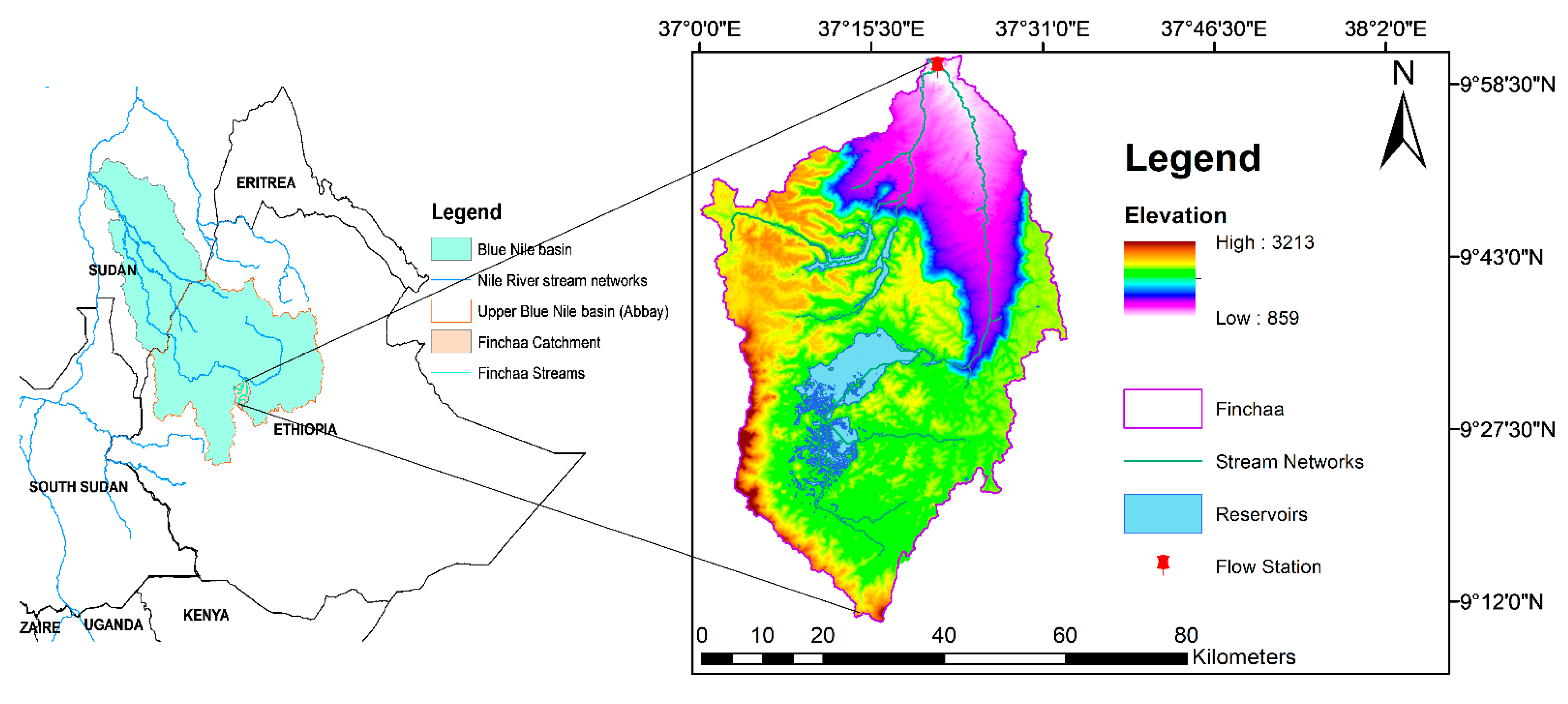
2.1. Study Area

Blue Nile is located between the 16°2′ and 7°40′ N latitudes and 32°30′ and 39°49′ E longitudes, with an estimated area of 311,437 km². It begins its flow from its source (Gish Abbay) in West Gojam northward as it joins Gilgel Abbay into Lake Tana and exits from the south-east of Lake Tana flowing to the south and then westward, cutting a deep gorge towards the western part of Ethiopia [28].

The Upper Blue Nile in Ethiopia (also called the Abbay Basin) has a number of tributaries, from which Finchaa was chosen for this particular study. The Finchaa catchment is located in the Western part of Ethiopia in Oromia Regional state between the 9°10′ to 10°00′ North latitudes and 37°00′ and 37°40′ East latitudes. The catchment is located around 315 km northwest of Addis Ababa the in Upper Blue Nile River basin, with three watersheds (Finchaa, Amerti and Neshe watersheds). The Finchaa and Neshe reservoirs were built primarily for hydropower generation while the Amerti reservoir was built to feed the Finchaa reservoir for more power generation through the Finchaa hydropower project. The description of the study area is shown by Figure 1.

Topographically, the Blue Nile basin is characterized by rugged and mountains features with altitude ranges varying from 859 m asl in the lowland valleys to 3213 m asl in the highlands around the upstream periphery of the catchment.

The land use/land cover of Finchaa catchment follows the divide between highland and lowland. In the past, the lowlands were predominantly covered with natural forest. But now the forests have been reduced to remnants, with the land having been converted for cultivation and irrigated agriculture. The highlands including the mountains area are dominantly under intensive agricultural cultivation [23]. The natural forests like Acacia-Commiphora deciduous wood, Acacia abyssinica, Acacia Senegal-gal (L.) Wild, Podocarpus falcatus, Cordial africana Lam, Ficus vasta Forssk and Carissa spinarum L. are being replaced by Eucalyptus globuls and Juniperus procera Hochst.

The catchment’s annual rainfall ranges from 1367 to 1842 mm with average annual rainfall of 1604 mm. The southern and western highlands of Finchaa receive annual rainfall higher than 1500 mm, while the northern lowlands receive lower rainfall. The catchment experiences peak rainfall from July to August [7].

2.2. Data Sources

Data

When modeling sediment yield, the integration of spatial and temporal data presented in

Table 1. Description of spatial and temporal data used in the SWAT model set up.

Data Types	Description	Source	Period/Scale
DEM	DEM was used to delineate the catchment and stream networks	Shuttle Radar Topography Mission (SRTM) 1 Arc-Second Global from https://earthexplorer.usgs.gov (accessed on 18 May 2021)	30 m
Soil	Soil data from a vector map was processed in to a 30 m raster. World digital soil map and soil grids were used to extract the Soil physico-chemical properties	Soil data processed from Ministry of Water, Irrigation and Electricity with digital soil map grids as presented by Dibaba et al. [20]	1:50,000 and 250 m grid
Land Use/Land Cover	Land use/land cover map of 2017 was used	LULC map derived from Landsat 8 OLI Dibaba et al. [23]	30 m
Weather	Daily rainfall, temperature, wind speed, relative humidity, solar radiation of 5 stations	National Meteorological Agency, Ethiopia (NMA)	1987–2015
Streamflow	Daily stream flow	Ministry of Water, Irrigation and Electricity, Ethiopia	1990–2007
Sediment Data	Daily sediment data	Ministry of Water, Irrigation and Electricity, Ethiopia	1990–2007

was used in a SWAT model. The Digital Elevation Model (DEM), soil, land use/land cover and weather data were used to develop a SWAT model set up. Streamflow and sediment data were used for model calibration and validation.

2.3. Methodology

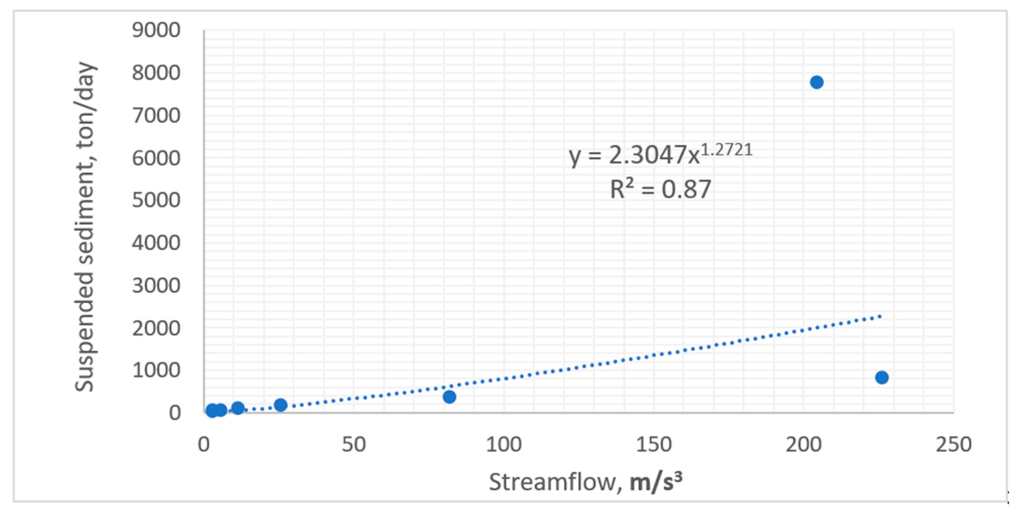
2.3.1. Sediment Rating Curve

The sediment load data collected from the Ministry of Water, Irrigation and Electricity (MoWIE) with the corresponding streamflow data are available only for a few days in a year. This is inadequate for analysis of hydrological model calibration and validation. In areas where no continuous-time step of suspended sediment records exists, estimates derived from empirical relations between the measured sediment records as a function of the corresponding streamflow were used [29]. Consequently, a sediment rating curve was developed to estimate the sediment yield from the flow measurements. Before developing the rating curve, the measured sediment load/concentration in mg/L was converted to the sediment yield (ton/day) using Equation (1).

Qs = 0.0864 ∗ Sc ∗ Qf

(1)

Then, curve fitting with a power function was developed for the regression model using the suspended sediment (Qs) and streamflow (Qf) with Equation (2)

Qs = a ∗ Qf^b

(2)

where Qs is the suspended sediment (ton/day), Sc is the suspended sediment concentration (mg/L), a and b are regression constants to be determined from the suspended sediment loads and observed streamflow. In this study, a and b were determined to be 2.3047 and 1.2721, respectively. The sediment rating curve is shown in Figure 2.

2.3.2. Best Management Practice Scenarios

Before the application of the BMPs scenarios, the SWAT model was validated and parameterized to examine the land management scenarios. Then, the approach of an estimation of what might happen under specific scenarios of BMPs against the baseline scenario was held. The evaluation was based on how the various BMPs simulate soil loss against the calibrated parameters of the SWAT hydrological model. The procedure involves two general steps: baseline simulation and the BMPs scenario simulations. The baseline values of the input parameters for evaluation of the BMPs scenarios could be selected through two procedures: model calibration procedures and suggested values from previous experiences or the literature [2,25,30] For this study, both strategies were combined: first the baseline values of the BMPs parameters were taken from the calibrated simulations of the SWAT hydrological model and then were compared with the literature suggestions.

The selection of BMPs and the values of their parameters are specific to the site topography, land use, soil and climate conditions and should reflect the reality of the study area [31]. In this context, applicable BMPs were selected from the community based Participatory Watershed Development Guideline of Ethiopia [32], SWC in Ethiopia-a review [3] and guidelines for development agents on SWC in Ethiopia [33]. Consequently, six BMPs scenarios that include a vegetative contour strip, soil/stone bund, contour farming, slope terracing, zero free grazing and reforestation were selected for the evaluation (

Table 2. Description of the BMPs scenarios and the parameter changes in the SWAT model.

Scenarios	Description	Parameter Name	Pre-BMP/Calibration Value	Post-BMP/Modified Value
Scenario 0	Baseline	Simulations with the calibrated model	-	-
Scenario 1	Grass contour strip	FILTERW	0	1 m
		USLE_P	0.53	0.34
		SLSUBBSN	*	0.50 *
		HRU_SLP	*	0.75 *
Scenario 2	Soil/stone bund	CN2.mgt	*	−3 *
		USLE_P	0.53	0.32
		SLSUBBSN	*	0.50*
Scenario 3	Contour farming	CN2	*	−3 *
		USLE_P	0.53	0.6 for slope 1–2% 0.5 for slope 3–8%
Scenario 4	Slope Terracing	CN2	*	−5 *
		USLE_P	0.53	0.12 for slope 1–2% 0.10 for slope 3–8%
Scenario 5	Zero free grazing	CN2	*	−2 *
		USLE_P	0.53	0.34
		USLE_C	0.51	0.05
		OV_N	0.14	0.19
Scenario 6	Reforestation	Is a management practice of land use change

* calibrated values.

). All the selected scenarios utilize locally available resources and they are agro-ecologically fit. Hence, they have a reasonable chance of being implemented in the Finchaa catchment.

Base scenario: the base scenario was represented by the actual/present conditions existing in the catchment.

Scenario 1 was represented by a vegetative contour strip. Vegetative contour strips are established along the contour on farmlands to filter surface runoff and trap sediment [2]. They are also used to counteract surface runoff [34]. Parameters modified in SWAT to simulate the effect grass contour strip include FILTERW, USLE_P, SLSUBBSN and HRU_SLP. The values of the parameters are presented in Table 2. The parameter value assignment was based on the experiences of local research in the Ethiopian highlands [2,26]. For the sake of comparison, filter strips with a 1 m strip were compared with vegetative contour strip.

Scenario 2 was represented by stone/soil bunds. The stone/soil bund is a sound practice for soil erosion control in the Ethiopian highlands [35]. This practice reduces runoff and soil loss by reducing the slope length and creating retention areas. The effect of stone/soil bund practice in the Finchaa catchment was simulated by modifying the curve number (CN2), slope length (SLSUBBSN) and management support practice factor (USLE_P) parameters. As presented by Table 2, the values of the stone/soil bund parameters were taken from the recommendations of previous studies [2,14,15,35]. Accordingly, CN2 was reduced by 3 units, SLSUBBSN reduced by 50% and USLE_P set to 0.32 for shrublands, grasslands and cultivated lands with slope classes higher than 8%.

Scenario 3 was assigned by contour farming. Contour farming is a practice of tillage and planting across a slope following the contour lines [30]. The practice helps to reduce surface runoff by impounding water in small depressions and through the reduction of sheet and rill erosion [25]. This scenario used a soil conservation service curve number (CN2) and management support practice factor (P-factor) to evaluate this practice in all agricultural lands. Contouring is most effective on land slopes of 3% to 8% [36,37]. The scenario was applied by modifying the parameter CN2, which was decreased by 3, and modifying the USLE_P with 0.6 and 0.5 based on the land slope [25,37,38].

Scenario 4 was assigned by slope terracing. Terraces are series of horizontal ridges made in a hillside that involve the construction of embankments and channels to control overland flow and conduct runoff to the safe outlet [36]. Terracing is more effective when combined with contour farming and other conservation practices [37]. Slope terracing was represented by a management support practice factor (P-factor) and soil conservation service curve number (CN2) across agricultural lands. The scenario was applied by modifying the parameters CN2, which was decreased by 5, and modifying USLE_P with 0.12 and 0.1 based on the land slope [25,37,38].

Scenario 5 was established by zero free grazing. Controlled grazing is the proper utilization of grasslands with livestock through avoiding degradation of vegetation and soil [33]. This scenario was represented in SWAT model by setting the USLE_P to 0.34, reducing CN2 by 2 and modifying the manning’s roughness coefficient for overland flow (OV_N) as 0.19 and reducing USLE_C to 0.05 [39,40].

Scenario 6 was established by reforestation of rangelands and croplands in excess of the 25% slope. Reforestation helps to reduce overland flow and rainfall erosivity by introducing land use change [13,26]. The practice was used by converting range lands and farmlands into forestland. Foresting the degraded agricultural fields is more feasible and practical than foresting all cultivated fields. Further, it is easy to identify degraded agricultural lands by farmers and most farmers have started plantation of Eucalyptus planting in degraded areas of their farmlands. In this scenario, 4% of rangeland and 4% of agricultural fields were replaced by mixed forest. The mixed forest was selected due to its dominant coverage in the catchment. The impact of reforestation was simulated by introducing land use/land cover in a land use update of the watershed data.

The effectiveness of the BMPs scenario was computed by calculating the percentage change in the model outputs using Equation (3).

$$\mathrm{Effectiveness} \mathrm{of} \mathrm{BMP}=\left(\frac{\mathrm{PreBMP}-\mathrm{Post} \mathrm{BMP}}{\mathrm{PreBMP}}\right)\ast 100$$

(3)

2.3.3. River Flow and Sediment Yield Modeling Approach

The conceptual physical-based model Soil and Water Assessment Tool (SWAT) was used to predict the impact of land management practices on river flow and soil loss [36]. In SWAT, a watershed is divided into multiple sub-watersheds, which are then further subdivided into the smallest unit for the catchment, which are called hydrologic response units (HRUs). The HRU is the smallest unit for the catchment physical process discretized based on the homogeneity of the land use, soil type and slope classes. The simulation of the hydrological components at each HRUs is based on the water balance equation [40] given in Equation (4).

$$\mathrm{SW}t=\mathrm{SW}o+{{\displaystyle \sum }}_{\mathrm{i}=1}^{\mathrm{t}}(\mathrm{R}day-\mathrm{Q}surf-\mathrm{E}a-\mathrm{W}seep-\mathrm{Q}gw)$$

(4)

where SWt is the final soil water content (mm), SWo is the initial water content (mm), t is the time (days), Rday is the amount of precipitation on day I (mm), Qsurf is the amount of surface runoff on day I (mm), Ea is the amount of evapotranspiration on day I (mm), Wseep is the amount of water entering the vadose zone from the soil profile on day I (mm) and Qgw is the amount of return flow on day I (mm).

SWAT uses the Modified Universal Soil Loss Equation (MUSLE) to estimate the sediment yield for each HRUs [36,41] using equation 5. In MUSLE, the prediction of sediment yield was improved compared to in USLE, since runoff is a function of antecedent moisture and rainfall energy.

Sed = 11.8 ∗ (Qsurf ∗ qpeak ∗ Areahru) 0.56 ∗ KUSLE ∗ PUSLE ∗ LSUSLE ∗ CUSLE ∗ CFRG

(5)

In Equation (5), Sed is the sediment yield (ton/day), Qsurf is surface runoff volume (mm/ha) qpeak is the peak surface runoff rate (m³/s), Areahru is the area of hydrologic response unit (ha), KUSLE is the USLE soil erodibility factor, PUSLE is USLE soil protection factors, LSUSLE is USLE topography factor, CUSLE is USLE topography factors cover and CFRG is the coarse fragment factor.

The Arc SWAT 2012 interface was used to parameterize and setup the model. On the basis of 30 m × 30 m DEM, land use/land cover and soil data, the Finchaa catchment was discretized into 25 sub-basins, which were further divided into 357 HRUs. Data of five weather stations located inside the catchment with one station considered as weather generator were used for the entire simulation period from 1987 to 2007.

2.3.4. Model Evaluation: Sensitivity Analysis, Calibration and Validation

The uncertainties of SWAT model prediction were analyzed using SWAT Calibration and Uncertainty Procedures (SWAT-CUP), which is the program for integrated sensitivity analysis, calibration and validations [42]. The Sequential Uncertainty Fitting (SUFI-2) in the SWAT-CUP was used for model sensitivity analysis, calibration and validation. Sensitivity analysis helps to identify parameters that strongly influence the flow process [43]. The global sensitivity analysis procedure was used for the evaluation of streamflow and sediment parameters’ relative sensitivity using the Latin hypercube ‘one-at-a-time’ regression systems. The coefficient of a parameter over its standard error (t-stat) was used for parameter sensitivity and ranking, while the significance of the sensitivity was determined by the p-value.

The capability of the SWAT model to accurately simulate the streamflow and sediment yield was tested through calibration and validation of the model. During calibration, model parameters were estimated by comparing the model prediction with the observed data for the same condition [43,44]. Then, validation was used to test the calibrated model without further parameter adjustments with an independent dataset. The length of the observed data record determined the time period for calibration and validation. When the observed data was not sufficiently long, the calibration period was considered sufficiently longer than the validation period. In this study, observed streamflow and sediment yield data obtained from the sediment rating curve were used to calibrate and validate the model from 1990 to 2007. The first three years were used for model warm-ups whereas two-third and one-third of the total data were used for calibration and validation, respectively.

As surface runoff directly affects the soil erosion, stepwise procedures for calibration of streamflow followed by sediment data were used [43,44]. First, we calibrated the streamflow parameters, then while keeping the calibrated parameters of streamflow, sediment parameters were calibrated.

The performance of the model simulation was determined by comparing the observed streamflow and sediment yield against their simulated data. Statistics like coefficients of determination (R²), Nash-Sutcliffe efficiency (NSE) and percent bias (PBIAS) were used to test the goodness of fit between the simulated and observed values. The model performance ratings were based on the statistics recommended by Moriasi et al. (44). R² varies between 0 and 1, where a higher value shows less error. NSE ranges from negative infinity to 1 (best). A negative value of PBIAS indicates overestimation, a positive value indicates underestimation and values close to 0 show that best parameter sets are found. These statistics were calculated using Equations (6)–(8)

$$R^2=\frac{{{\displaystyle \sum }}_{i=1}^n{\left[\left(Qobs-Q\overline{o}bs\right)\left(Qsim-\overline{Q}sim\right)\right]}^2}{\sqrt{{{\displaystyle \sum }}_{i=1}^n{\left(Qobs-\overline{Q}obsm\right)}^2{{\displaystyle \sum }}_{i=1}^n{\left(Qsim-\overline{Q}sim\right)}^2}};0\le R^2\le 1$$

(6)

$$NSE=1-\frac{{{\displaystyle \sum }}_{i=1}^n{\left(Qobs-Qsim\right)}^2}{{{\displaystyle \sum }}_{i=1}^n{\left(Qobs-Q\overline{o}bs\right)}^2};-\infty \le NSE\le 1$$

(7)

$$PBIAS=100\%\left(\frac{{{\displaystyle \sum }}_{i=1}^{n}Qobs-{{\displaystyle \sum }}_{i=1}^{n}Qsim}{{{\displaystyle \sum }}_{i=1}^{n}Qobs}\right)$$

(8)

where Qobs is the measured discharge, Qsim is the simulated discharge, $\overline{\mathrm{Q}}\mathrm{obs}$ is the average measured discharge and $\overline{\mathrm{Q}}\mathrm{sim}$ is the average simulated discharge.

3. Results

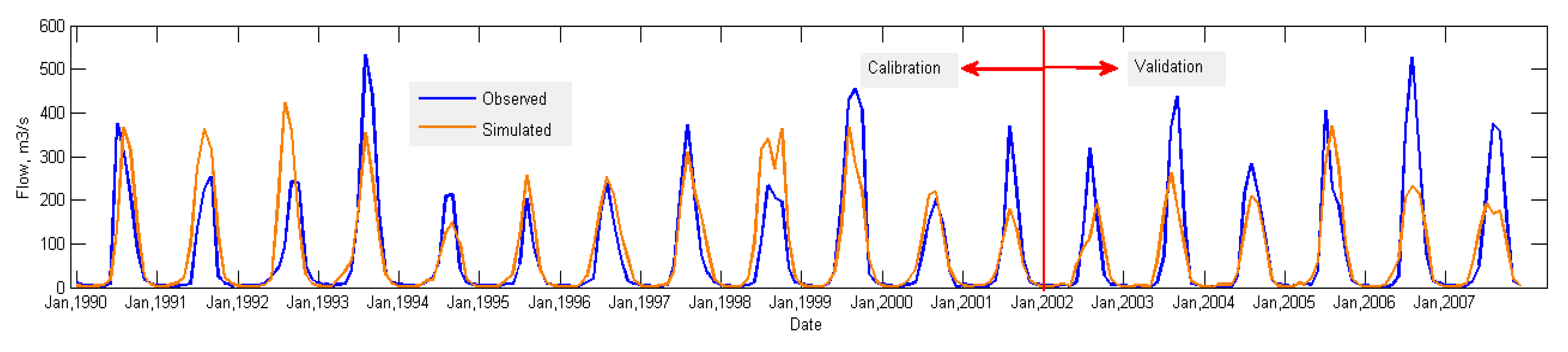
3.1. Sensitivity Analysis, Calibration and Validation

Monthly streamflow and sediment data at the outlet of the catchment was used for model calibration and validation. Prior to calibration, model sensitivity analysis was done based on p-values and t-stat. Lower p-values and larger absolute t-stat indicate the most significant parameter and increased sensitivity of the parameter. Accordingly, the top 5 most sensitive parameters for streamflow were the SCS curve number (CN2), Baseflow alpha-factor (ALPHA_BF), Manning’s ‘n’ value for the main channel (CH_N2), the Soil evaporation compensation coefficient (ESCO) and Available water capacity of the soil layer (SOL_AWC).

The sensitive parameters for sediment parameters were the USLE support practice factor (USLE_P), Exponential factor for sediment routing (SPEXP), Channel erodibility factor (CH_COV1), Linear factor for channel sediment routing (SPCON) and Channel cover factor (CH_COV2). SCS curve number (CN2) was found to be sensitive to both streamflow and sediment yield. These parameters were calibrated with the recommended ranges shown in

Table 3. Calibration flow parameter statistics, lower and upper boundary range, sensitivity rank and optimized parameter values using SUFI-2.

	Parameter	Description	Range	Fitted Value	Rank
Stream Flow	1:R__CN2.mgt	SCS curve number	± 25%	−0.65%	1
	2:V__ALPHA_BF.gw	Base flow recession constant	0–1	0.252	2
	6:V__CH_N2.rte	Manning’s n value for the main channel	0–0.3	0.0188	3
	3:V__ESCO.hru	Soil evaporation compensation coefficient	0–1	0.7376	4
	4:R__SOL_AWC(..).sol	Available water capacity of the soil layer	±25%	1.19%	5
	10:V__SLSUBBSN.hru	Average slope length	10–150	30.64	6
To	8:R__SOL_K(..).sol	Saturated hydraulic conductivity	±25%	4.07%	7
Sediment Yield	12:V__USLE_P.mgt	USLE support practice factor	0–1	0.53	1
	13:V__SPEXP.bsn	Exponential factor for sediment routing	1–2	1.27	2
	15:V__CH_COV1.rte	Channel erodibility factor	0.01–0.6	0.471	3
	14:V__SPCON.bsn	Linear factor for channel sediment routing	0.0001–0.01	0.0018	4
	16:V__CH_COV2.rte	Channel cover factor	0.001–1	0.456	5

and used to compute the amount of soil erosion from the catchment and the channel. The most sensitive sediment parameters found in this study are also reported by other studies in the Upper Blue Nile basin [2,13].

The model performance rating criteria showed a good agreement between the simulated and measured monthly streamflow. The R² value amounts to 0.68 and 0.72 and NSE value to 0.65 and 0.67 during calibration and validation, respectively. The PBIAS result shows a good performance of the model with slight overestimation (-ve) during calibration and satisfactory performance with underestimation (+ve) during the validation (

Table 4. Streamflow calibration and validation statistics using SUFI-2 at outlet 1.

Process	R2	NSE	PBIAS
Calibration	0.68	0.65	−11.7
Validation	0.72	0.67	18.1

).

The graphical analysis of the simulated and observed streamflow during calibration and validation indicated that SWAT model prediction is adequate over the ranges of streamflow (Figure 3). However, the model was unable to predict the peak flow in most of the calibration years and the model fully underestimated the peak flow throughout the validation years. The rising and falling limbs of streamflow were well simulated in most of the calibration and validation years.

The model performance rating criteria for the simulated and observed sediment yield showed R² values of 0.59 and 0.72 and NSE values of 0.57 and 0.71 for calibration and validation, respectively (

Table 5. Sediment yield calibration and validation statistics using SUFI-2 at outlet 1.

Process	R2	NSE	PBIAS
Calibration	0.59	0.57	−0.9
Validation	0.72	0.71	6.9

). The negative value of PBIAS showed a slight overestimation of the sediment load and a positive value of PBIAS for validation showed underestimation of the predicted sediment yield. Overall, the PBIAS value indicated that the SWAT model is very good for simulating the sediment yield.

The graphical analysis of the simulated and observed sediment yield indicated both overestimation and underestimation of the sediment simulation during calibration and underestimations during validation (Figure 4). The SWAT model was unable to predict the peak sediment in most of the calibration and validation years. It can be concluded that the model is good enough to simulate the rising and falling limb during both calibration and validation. If the peak flows can be simulated error free, then less deviations of simulated sediment yield can be expected.

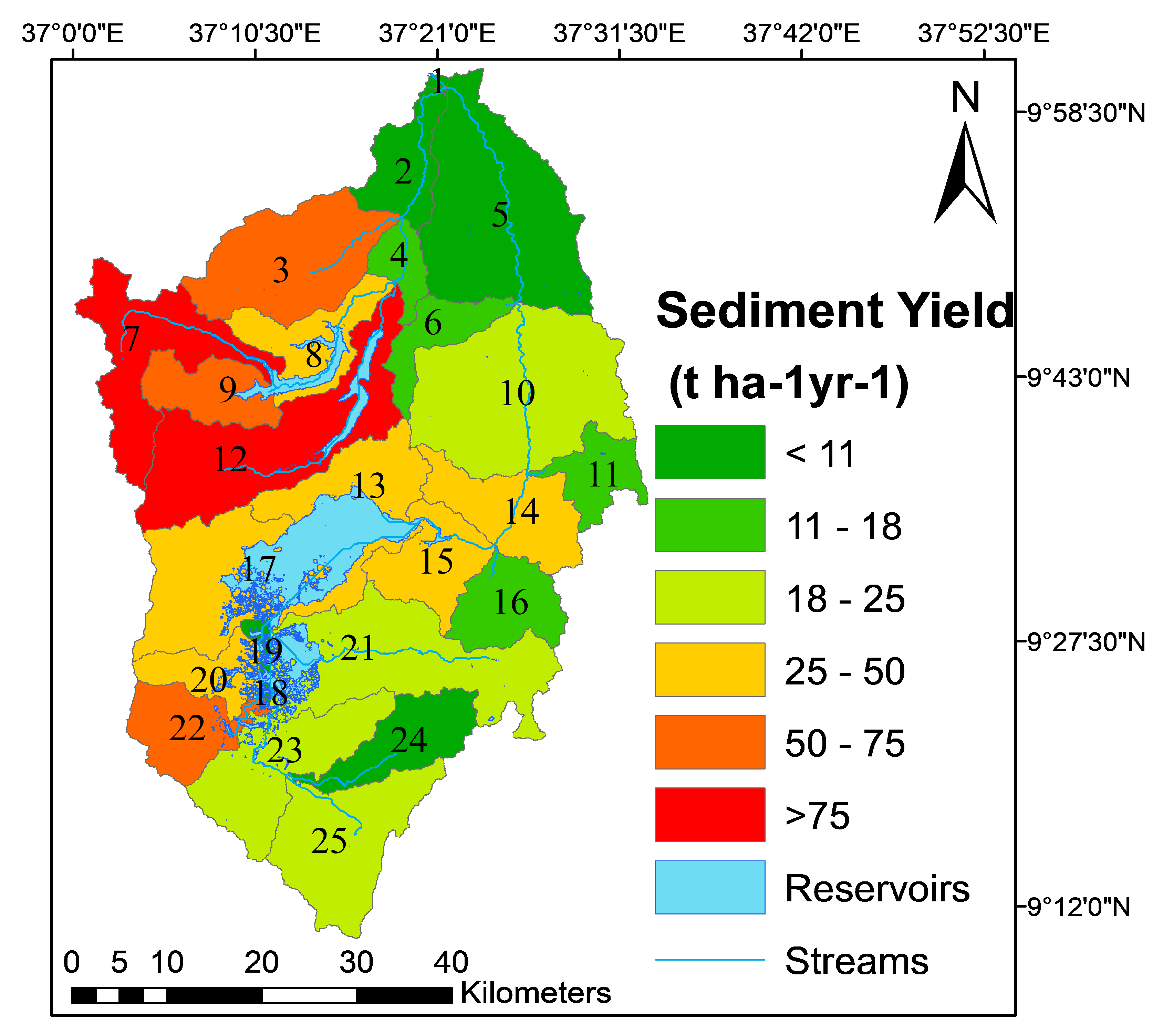
3.2. Watershed Prioritization to Sediment Yields in Finchaa Catchment

On the bases of the annual soil loss estimates, the simulation of the annual sediment yield in Finchaa catchment varies from 0.01 to 107.2 t ha⁻¹yr⁻¹ with an average SY of the whole catchment estimated to be 36.47 t ha⁻¹ yr⁻¹. To understand the prioritization and classification of the SY severity, the Finchaa catchment was classified into six erosion severity classes, as shown in

Table 6. Annual soil erosion and its severity.

Soil Loss- t ha−1yr−1	Severity	Area in ha	Area in Percent
<11	Low	49,481.9	15.0
11–18	Moderate	25,576.6	7.8
18–25	High	92,982.8	28.3
25–50	Very high	79,073.1	24.1
50–75	Severe	37,422.4	11.4
>75	Very severe	44,161.3	13.4

. The soil classes were defined based on the research experiences in Ethiopia [2,3,6]. Accordingly, 24.83% of the areas were predicted to suffer from severe to very severe erosion risks, which are in excess of 50 t ha⁻¹ yr⁻¹. About 48.89% of the catchment was estimated to from suffer very high to very severe soil erosion risks, which is are excess of 25 t ha⁻¹yr⁻¹.

The spatial distribution of land use/land cover types, soil types, slope, precipitation and temperature were used to elucidate the spatial distribution of sediment yield (SY) in the Finchaa catchment. The predicted average annual SY of the sub-basins using SWAT was used to map the soil erosion hotspot areas. Consequently, the lowest SYs which could be found in low-risk areas were predicted around the downstream and the highest SYs around the northwestern part of the catchment (Figure 5). The areas with severe and very severe soil loss are located in the northwestern part of the catchment where the steep slope lands are highly cultivated and overgrazed on the upstream of the Neshe and Amerti reservoirs. As presented in Figure 5, the majority of the sub-watersheds require the implementation of different types of soil and water conservation practices. However, since all sub-watersheds face equal risks of soil erosion, it is impossible to apply the watershed management practices at the same time for the whole catchment. In this context, the sub-watersheds that are at a greater risk of soil erosion should be prioritized first for treatment to achieve sustainable development of land and water resources.

Prioritization of sub-watersheds involves the ranking of the sub-watersheds according to the SY of each sub-basin and their vulnerability to the risk of soil loss severity. Accordingly, five sub-watersheds out of 25 fell under severe and very severe soil erosion risks (sub-basin labels of 7, 12, 3, 9 and 22) (Figure 5). Sub-basins 1, 2, 5, 18, 19 and 24 were predicted to face a low risk of soil loss severity and these sub-watersheds can be considered as the least prioritized areas.

3.3. BMPs Scenario Analysis in Finchaa Catchment

The application of different BMPs showed promising results for SY reduction (Figure 6). The application of filter strip alone reduced SY to 23.16 t ha⁻¹ yr⁻¹, which is equivalent to 36.47%. In this study, the application of vegetative contour strips with different grasses that reduces the overland slope led to a greater reduction of SY compared to a filter strip alone. Consequently, the simulation of vegetative contour strip showed a reduction of the SY by 63.9%. The BMPs scenarios were represented in Figure 6 as follows, grass contour strip-GS, soil/stone bund-SB, contour farming- CF, slope terracing- ST, zero free grazing- FG and reforestation-R.

The scenario of soil/stone bund reduced the SY to 12.826 t ha⁻¹ yr⁻¹, which is equivalent to 64.8% from the current SY. The simulation of contour farming and slope terracing in agricultural lands showed a reduction of SY to 30.23 t ha⁻¹ yr⁻¹ and 25.43 t ha⁻¹ yr⁻¹ which is equivalent to 17.1% and 30.3% reductions, respectively. It can be observed that slope terracing is more effective than contour farming.

Reforestation was evaluated by converting the croplands and rangelands in steep slope areas to plantations forests and its implementation reduced the SY to 24.40 t ha⁻¹ yr⁻¹, which is equivalent to a 33% reduction. A zero free grazing scenario reduced the SY to 20.50 t ha⁻¹ yr⁻¹, which is equivalent to 43.8%.

4. Discussion

The Gauging station in the Finchaa catchment is only available at a single outlet. Hence, streamflow and sediment calibration and validation were conducted only at a single station outlet of the catchment. Although the SWAT model was capable of estimate the sediment yields, reliability of the model is dependent on the availability of long-term data sets. In Ethiopia, the long-term sediment data is very limited and even large perennial rivers including streams in Finchaa only have a limited record of sediment data. In this context, the use of a sediment rating curve with a strong correlation (R² = 0.87) between the measured sediment data and runoff was used to generate the sediment data from the limited records of the sediment sample and its corresponding streamflow. The statistical figures (Table 4 and Table 5) and hydrographs (Figure 3 and Figure 4) used for performance evaluation of the SWAT in simulating the streamflow and sediment yield revealed that SWAT model prediction is adequate over the ranges of streamflow and sediment yield. Similarly, Betrie et al. [13] also reported that the fit between the sediment predictions and the observed sediment data showed good agreement at the El Diem gauging station for the whole Upper Blue Nile basin. A similar sediment rating curve approach was used by Gharibdousti et al. [45] to generate sediment data for SWAT model calibration and validation, where the sediment data from the observations was limited.

In the Finchaa catchment, the SWAT model was unable to predict the peak flow in most of the calibration and validation years. The deviations between observed and simulated peaks of sediment yields were comparable to those of peak flow. This finding was consistent with other research reports [45,46]. According to Zeiger and Hubbart [46], underestimation of the peak flows by SWAT model leads to underestimation of sediment peak. Further, Gharibdousti et al. [45] reported that the largest errors in sediment prediction were associated with errors of peak flow estimation due to the second storm effect problem in the SWAT model.

A sediment rating curve equation for sediment data generation was used to evaluate the model’s error, which could be associated with the data scarcity and streamflow data. In the Finchaa catchment, the relatively lower statistics of R² and NSE during sediment calibration could be related to the sediment rating curve equation, scarcity and quality of the data and stream flow process. In this context, following a low-error simulation of peak flow is the key factor for low-error simulation of sediment peaks. In general, the SWAT model is good enough to simulate the rising and falling limbs, both during the calibration and validation of the streamflow and sediment yield. The PBIAS statistics in both cases shows that the model slightly over estimates streamflow and sediment yield during calibration and underestimates during the validation.

The assessment of SY variations of an area helps to identify the areas where soil loss can be tolerated and to identify the hotspot areas. Actually, tolerable soil loss is the factor that maintains ecosystem service without degrading the capacity of soil to deliver services in the future [12]. The range of tolerable soil loss level in different agro-ecological conditions of Ethiopia is 2 to 18 t ha⁻¹ yr⁻¹ [39]. The other study reported tolerable ranges on crop production maintenance range from 1 to 11 t ha⁻¹ yr⁻¹ [12]. In this regard, only 15.05% of the catchment showed a tolerable rate of soil loss for maintenance of crop production as per FAO [12], whereas it was about 22.83% of the area according to Hurni [39]. This shows how far soil erosion risks are beyond the tolerable soil loss values in the catchment.

The area of lands characterized by the lowest SY were associated with those having good vegetation cover. Meanwhile, areas that were characterized by high SY were associated with the highest surface runoff from the highly cultivated crop fields with strongly rolling and hilly slopes. As presented by Figure 5, soil erosion risk is lower in areas with a good natural vegetation cover in the downstream of the catchment. A high risk of soil erosion was estimated around the southeastern catchment area, the upstream part of the catchment and downstream areas of the Neshe and Amerti reservoirs, whereas upstream and downstream areas of the Fincha reservoir were predicted to suffer from a very high risk of soil erosion. This finding is in contrast with the study by Ebabu et al. [9] who reported that erosion is higher in the midland than in the highland and lowland agro-ecologies. The high risk of SY on the upstream high lands of the catchment could be related to the uncontrolled activities of the community on the upstream areas and conversion of natural vegetation into croplands. According to Dibaba et al. [23], the communities displaced from the reservoir areas were forced to settle on the upstream highland areas. The uncontrolled activities of these community due to the limited land changed the forest and vegetation cover areas into highly cultivated lands. The steep slope nature of the lands added with the above-mentioned factors made the area generate high soil loss risks.

Comparing the spatial patterns and the estimates of the soil loss rate with what is observed from field plots, the spatial estimate is widely realistic. Based on field assessment of soil loss using the assessment of current erosion damage (ACED) on two sub-watersheds in the Finchaa catchment, the annual soil loss ranged from 24 to 160 t ha⁻¹ yr⁻¹ [22]. However, the ACED method does not account for the amount of soil loss contributed to by inter rill erosion. Further, the assessment of the soil loss based on field plots was only dependent on a few years of records and it may not be representative enough of long-term measurements. Higher estimates of annual soil loss relative to hydrological units or even whole catchments using the SWAT model are in line with the reports by FAO [12], who provided field plots with estimates of higher soil loss than the regional models. However, the study of soil loss based on the broader catchment/landscape is more effective than either plot or field scaled bases to address the land degradation related to erosion. The estimates of the SY in the Finchaa catchment was consistent with other studies in the upper Blue Nile basin. The simulation of SY using SWAT over the whole Upper Blue Nile basin shows that the SY varies from negligible to over 150 t ha⁻¹ [13]. Ayele et al. [47] in Koga catchment, a tributary to Gilgel Abay, the headwater of Blue Nile, reported the annual average SY to be 24.3 t ha⁻¹ yr⁻¹. On the same watershed (Koga watershed), Gelagay and Minale [48] reported that the average soil loss rate varies from 0 to 265 t ha⁻¹ yr⁻¹ with a mean annual soil loss value of 47.7 t ha⁻¹ yr⁻¹. SY in Lake Tana Basin varies from negligible to 169.3 t ha⁻¹yr⁻¹ with an annual average SY of 32 t ha⁻¹ yr⁻¹ [2]. Bewket and Teferi [49] in the Chemoga watershed reported annual soil loss from 0 to over 125 t ha-1yr-1 with average annual estimates for the whole watershed to be 93 t ha⁻¹yr⁻¹. Geleda watershed of Blue Nile basin showed the estimates of mean annual soil loss varies from 0 t ha⁻¹ yr⁻¹ in plain areas to 237 t ha⁻¹yr⁻¹ in the hilly terrains with an average soil loss of 23.7 t ha⁻¹ yr⁻¹ [50]. Yesuph and Dagnew [51] also reported an annual soil loss rate of Gedalas watershed from 0 to 935 t ha⁻¹ yr⁻¹ with a mean annual loss of 37 t ha⁻¹ yr⁻¹ for the watershed and 51 t ha⁻¹ yr⁻¹ for the crop fields.

In all case studies, the highest soil loss was reported from crop fields. This, however, is in contrast to Ebabu et al. [9], who reported higher SY from intensively grazed lands than from croplands. Higher estimates of soil loss [47,48,49,50,51,52] were reported when the soil loss prediction was conducted with RUSLE. The strength of RUSLE for soil loss prediction is higher in regions where data are scarce. However, it is questionable to use RUSLE in mountain terrains with steep slopes, as the soil loss estimates of RUSLE reports higher values due to the higher topographic factor LS. Major evidence for this is the great variation of soil loss estimation in Koga published by Ayele et al. [47] (24.3 t ha⁻¹yr⁻¹ using SWAT) and Gelagay and Minale [48] (47.7 t ha⁻¹yr⁻¹ using RUSLE). This is in line with FAO [12], who reported that the soil loss estimates vary substantially depending on the method used to derive them.

The simulation of spatial SY in the Finchaa catchment (0.01 to 107.2 t ha⁻¹yr⁻¹) was comparable with similar studies in the Ethiopian high lands. Berihun et al. [6] reported 13.17 to 95.01 t ha⁻¹ in Kecha and laguna watersheds in the Blue Nile basin. Relatively, the higher average soil loss in the Finchaa catchment (36.47 t ha⁻¹yr⁻¹) could be attributed to a steep slope with high mountains, intensive cultivation and higher rainfall in the Finchaa catchment.

There are few studies about the overall national or regional soil loss rate in Ethiopia. Sonneveld et al. [52] used a combination of different models to estimate the annual soil loss and the result varied from 0 t ha^-1 yr^-1 in the eastern and southeastern parts to 100 t ha⁻¹ yr⁻¹ in the northwestern part of the country. However, the causes of the spatial variations were not mentioned in the study. Another study also estimated the average SY from sheet and rill erosion of croplands in the Ethiopian highlands to be above 100 t ha⁻¹ yr⁻¹ [53]. Based on this study, 5.25% of the area in the Finchaa catchment experiences SY above 100 t ha^-1 yr^-1.

Research experience showed that there is an increase in study reports on soil erosion and sediment yield with evaluation of different soil and water conservation practices using the SWAT model in different parts of the world. The study by Mosbahi and Benabdallah [54] reported that SWAT model was capable of identifying the optimal management practice under a specific land use in a Tunisian semi-arid catchment. The SWAT model was used to evaluate the effectiveness of contour farming and filter strips on ecosystem services in the Thika-Chania catchment, Kenya [55]. Similarly, Gharibdousti et al. [45] showed that SWAT model can be used to prioritize feasible BMPs on fields in agriculture-pasture intensive watersheds, Southwestern Oklahoma, USA. SWAT was used to identify the sediment sources in a Mediterranean watershed [56].

However, the severity of the sediment yield varies along a region. Mosbahi and Benabdallah [54] classified soil loss severity as high when the sediment yield is in the range of 10-20 t ha^-1 yr^-1 and very high when the yield exceeds 20 t ha⁻¹ yr⁻¹ in semi-arid areas. A high erosion rate is reported for when a sediment yield ranges from 7 to 13 t ha⁻¹yr⁻¹ in the Carapelle watershed, Northern Apulia [56]. The research report by Ricci et al. [56] revealed that the highest erosion rates were generated from upstream areas characterized by steep slopes.

The performance of BMPs in reducing sediment yield of the Finchaa catchment is comparable to the results reported by Demissie et al. [26], with a reduction of SY by 35% after the application of filter strips. Betrie et al. [13] for the Upper Blue Nile also reported SY reduction ranges from 29% to 68% due to the application of filter strips. The SY reduction by soil/stone bund (64.8%) was comparable with the reduction of SY by 68% reported by Gebremichael et al. [15] in field-scale and 61% SY reduction in the Lake Tana Basin reported by Lemma et al. [2].

Like the magnitude of the sediment yields, the performance of BMPs varies along different regions. The highest sediment yield reduction by parallel terraces compared to contour farming and reforestation was reported in the Tunisian semi-arid region [54]. Although the magnitude of the reduction varied, terracing was also reported with higher sediment yield reduction compared to contour farming in the Finchaa catchment. Similarly, Gathagu et al. [55] reported higher SY reduction by filter strip compared to contour farming.

Although the contour farming, slope terracing, zero free grazing and reforestation are significant in reducing the SY, the yield is still above the tolerable soil loss. This shows that the BMPs scenario should be supported with other soil and land management measures like biological ones. The higher sediment yield reduction by stone bund and a vegetative contour strip could be related to their wider implementation in the catchment.

In the Finchaa catchment, the limited and slower response to the multifaceted issues of communities and the need for integration and comprehensive action are exacerbating environmental problems. In this regard, the outcome of this study could help decision makers, stakeholders and water resource planners, as it provides clues on how prioritization of hot spot areas could facilitate proactive natural resource management. It also helps the efforts of introducing best practices towards natural resources management options like integrated water and soil conservation practices. For the effective application of the identified BMPs, this study could help with identifying gaps for proper soil and water management practices that should be in place on the ground. In most cases, the development of interventions in Ethiopia avoids in-depth analysis and understanding of the environment-population nexus. Consequently, necessary collaboration and coordination in designing and implementing comprehensive and integrated development interventions that can support sustainable development in a fullest sense need attention and focus from all concerned actors. However, there is no sort of organizational structure at the grassroots level, for instance a watershed committee for watershed conservation at a local/community level in a catchment. Moreover, experiences showed that watershed managements were problematic when applied without community participation and only using hydrological planning units. This shows that a poorly planned watershed approach without an integrative approach of a hydrology and socio-ecological process could result in complete failure.

Although the study result provided information regarding the importance of applying BMPs for sediment yield reduction, the economic consideration of the management practices should be considered to select the most cost effective BMPs for the feasibility of the management scenarios. The evaluation of different BMPs in this study was held with respect to the present condition. However, study on how the BMPs continue to perform under the future climate change scenarios is required to achieve sustainable soil and water management in the future.

5. Conclusions

Both statistical analysis and the hydrographs of simulated and observed streamflow and sediment yield through calibration and validation revealed that the SWAT model is capable of simulating the hydrological regime of the Finchaa catchment. The simulation of the annual SY in the catchment varies from 0.01 around the downstream of the catchment to 107.2 t ha⁻¹ yr⁻¹ around the northwestern part, with an average SY of the whole catchment estimated to be 36.47 t ha⁻¹yr⁻¹.

The annual soil loss estimates in the Finchaa catchment were classified into six erosion severity classes, with the majority of the area (48.89%) being classified to suffer very high to very severe soil erosion risks. The areas with severe and very severe soil loss are located in the northwestern part of the catchment where the steep slope lands are highly cultivated around the Neshe reservoir. Additionally, 15.05% of the catchment falls under the category of tolerable soil loss for maintenance of crop production and the areas are characterized with good natural vegetation covers in the downstream of the catchment.

This research attempted to determine the potential soil erosion sources for prioritization and evaluation of best management practices in the Finchaa catchment. The result shows that not all sub-watersheds were found to be under equal risk of soil erosion. In this regard, prioritization enabled us to identify sub-watersheds that are at a greater risk of soil erosion in the catchment. The areas under high risk of soil erosion classified as severe and very severe are characterized by steep slope and intensive cultivation. Further, the areas are characterized by poor vegetation cover. Generally, croplands and slope are the dominant factors for the simulation of high sediment yield. Sub-basins that were predicted to face a low risk of soil loss are considered as the least prioritized areas. The majority of the list prioritized areas are characterized by good vegetation cover and are located at lowlands of the catchment. Comparatively, the upstream areas have more serious soil erosion than the lowland areas of the catchment.

The application of different BMPs showed promising results of SY reduction, with the highest reduction simulated by vegetative contour strip and soil bund scenarios, whereas the lowest reduction was reported by contour farming. Our finding suggests that the application of some BMPs requires further soil and land management measures like biological measures to achieve the tolerable soil loss limit. In general, the study proved that prioritizations are important not only to identify erosion hotspots but also to identify the most effective BMPs.

In general, the study has made an effort to provide new and updated insights at a watershed level on management options that can facilitate more proactive approaches to maintain the soil and land health through reversing degradation risks in the Finchaa catchment. This is important in relation to the assessments of the BMPs resilience and could facilitate the adoption of different BMPs to control soil loss, allowing water resources to regenerate. Applying appropriate management practices on degraded areas and sloppy lands could enhance groundwater recharge and surface runoff, which washes the topsoil into the reservoirs. This eventually helps to sustain land, water and the life span of reservoirs.

References

1. Arsano, Y. Ethiopia and the Nile Dilemmas of National and Regional Hydropolitics; University of Zurich: Zurich, Swezerland, 2007. [Google Scholar]
2. Lemma, H.; Frankl, A.; van Griensven, A.; Poesen, J.; Adgo, E.; Nyssen, J. Identifying erosion hotspots in Lake Tana Basin from a multisite Soil and Water Assessment Tool validation: Opportunity for land managers. Land Degrad. Dev. 2019, 30, 1449–1467. [Google Scholar] [CrossRef] [Green Version]
3. Haregeweyn, N.; Tsunekawa, A.; Nyssen, J.; Poesen, J.; Tsubo, M.; Tsegaye Meshesha, D.; Schütt, B.; Adgo, E.; Tegegne, F. Soil erosion and conservation in Ethiopia: A review. Prog. Phys. Geogr. 2015, 39, 750–774. [Google Scholar] [CrossRef] [Green Version]
4. Dabi, N.; Fikirie, K.; Mulualem, T. Review Article Soil and Water Conservation Practices on Crop Productivity and its Economic Implications in Ethiopia: A Review. Asian J. Agric. Res. 2017, 11, 128–136. [Google Scholar] [CrossRef] [Green Version]
5. Adimassu, Z.; Langan, S.; Johnston, R.; Mekuria, W.; Amede, T. Impacts of Soil and Water Conservation Practices on Crop Yield, Run-off, Soil Loss and Nutrient Loss in Ethiopia: Review and Synthesis. Environ. Manag. 2017, 59, 87–101. [Google Scholar] [CrossRef] [PubMed]
6. Berihun, M.L.; Tsunekawa, A.; Haregeweyn, N.; Dile, Y.T.; Tsubo, M.; Fenta, A.A.; Meshesha, D.T.; Ebabu, K.; Sultan, D.; Srinivasan, R. Evaluating runoff and sediment responses to soil and water conservation practices by employing alternative modeling approaches. Sci. Total Environ. 2020, 747, 1–18. [Google Scholar] [CrossRef]
7. Dibaba, W.T.; Miegel, K.; Demissie, T.A. Evaluation of the CORDEX regional climate models performance in simulating climate conditions of two catchments in Upper Blue Nile Basin. Dyn. Atmos. Ocean. 2019, 87, 1–14. [Google Scholar] [CrossRef]
8. Dile, Y.T.; Tekleab, S.; Ayana, E.K.; Gebrehiwot, S.G.; Worqlul, A.W.; Bayabil, H.K.; Yimam, Y.T.; Tilahun, S.A.; Daggupati, P.; Karlberg, L.; et al. Advances in water resources research in the Upper Blue Nile basin and the way forward: A review. J. Hydrol. 2018, 560, 407–423. [Google Scholar] [CrossRef]
9. Ebabu, K.; Tsunekawa, A.; Haregeweyn, N.; Adgo, E.; Meshesha, D.T.; Aklog, D.; Masunaga, T.; Tsubo, M.; Sultan, D.; Fenta, A.A.; et al. Effects of land use and sustainable land management practices on runoff and soil loss in the Upper Blue Nile basin, Ethiopia. Sci. Total Environ. 2019, 648, 1462–1475. [Google Scholar] [CrossRef]
10. Tully, K.; Sullivan, C.; Weil, R.; Sanchez, P. The State of Soil Segradation in Sub-Saharan Africa: Baselines, Trajectories, and Solutions. Sustainability 2015, 7, 6523–6552. [Google Scholar] [CrossRef] [Green Version]
11. Nkonya, E.; Mirzabaev, A. Economics of Land Degradation and Improvement—A Global Assessment for Sustainable Development; Springer International Publishing: Cham, Switzerland, 2016; Available online: http://link.springer.com/10.1007/978-3-319-19168-3 (accessed on 13 March 2021).
12. FAO. Soil Erosion: The Greatest Challenge to Sustainable Soil Management; FAO: Rome, Italy, 2019. [Google Scholar]
13. Betrie, G.D.; Mohamed, Y.A.; Van Griensven, A.; Srinivasan, R. Sediment management modelling in the Blue Nile Basin using SWAT model. Hydrol. Earth Syst. Sc. 2011, 15, 807–818. [Google Scholar] [CrossRef] [Green Version]
14. Sultan, D.; Tsunekawa, A.; Haregeweyn, N.; Adgo, E.; Tsubo, M.; Meshesha, D.T.; Masunaga, T.; Aklog, D.; Ebabu, K. Analyzing the runoff response to soil and water conservation measures in a tropical humid Ethiopian highland. Phys. Geogr. 2017, 38, 423–447. [Google Scholar] [CrossRef]
15. Gebrernichael, D.; Nyssen, J.; Poesen, J.; Deckers, J.; Haile, M.; Govers, G.; Moeyersons, J. Effectiveness of stone bunds in controlling soil erosion on cropland in the Tigray Highlands, northern Ethiopia. Soil Use Manag. 2005, 21, 287–297. [Google Scholar] [CrossRef]
16. Taye, G.; Vanmaercke, M.; Poesen, J.; Van Wesemael, B.; Tesfaye, S.; Teka, D.; Nyssen, J.; Deckers, J.; Haregeweyn, N. Determining RUSLE P -and C -factors for stone bunds and trenches in rangeland and cropland, North Ethiopia. Land Degrad. Dev. 2018, 29, 812–824. [Google Scholar] [CrossRef]
17. Mengistu, F.; Assefa, E. International Soil and Water Conservation Research Farmers’ decision to adopt watershed management practices in Gibe basin, southwest Ethiopia. Int. Soil Water Conserv. Res. 2019, 7, 376–387. [Google Scholar] [CrossRef]
18. Teshome, A.; Rolker, D.; De Graaff, J. Financial viability of soil and water conservation technologies in northwestern Ethiopian highlands. Appl. Geogr. 2013, 37, 139–149. [Google Scholar] [CrossRef]
19. Schmidt, E.; Tadesse, F. The impact of sustainable land management on household crop production in the Blue Nile Basin, Ethiopia. Land Degrad. Dev. 2019, 30, 777–787. [Google Scholar] [CrossRef] [Green Version]
20. Dibaba, W.T.; Demissie, T.A.; Miegel, K. Watershed Hydrological Response to Combined Land Use/Land Cover and Climate Change in Highland Ethiopia: Finchaa Catchment. Water 2020, 12, 1801. [Google Scholar] [CrossRef]
21. Kositsakulchai, E.; Ayana, A.B.; Edossa, D.C. Simulation of Sediment Yield using SWAT Model in Fincha Watershed, Ethiopia. Nat. Sci. 2012, 46, 283–297. [Google Scholar]
22. Tefera, B.; Sterk, G. Land management, erosion problems and soil and water conservation in Fincha’a watershed, western Ethiopia. Land Use Policy 2010, 27, 1027–1037. [Google Scholar] [CrossRef]
23. Dibaba, W.T.; Demissie, T.A.; Miegel, K. Drivers and Implications of Land Use/Land Cover Dynamics in Finchaa Catchment, Northwestern Ethiopia. Land 2020, 9, 113. [Google Scholar] [CrossRef] [Green Version]
24. Addis, H.K.; Abera, A.; Abebaw, L. Economic benefits of soil and water conservation measures at the sub-catchment scale in the northern Highlands of Ethiopia. Prog. Phys. Geogr. 2019, 44, 1–16. [Google Scholar] [CrossRef]
25. Arabi, M.; Frankenberger, J.R.; Engel, B.A.; Arnold, J.G. Representation of agricultural conservation practices with SWAT. Hydrol. Process. 2007, 22, 3042–3055. [Google Scholar] [CrossRef]
26. Demissie, T.A.; Saathoff, F.; Seleshi, Y.; Gebissa, A. Evaluating the Effectiveness of Best Management Practices in Gilgel Gibe Basin Watershed-Ethiopia. J. Civ. Eng. Archit. 2013, 7, 1240–1252. [Google Scholar]
27. López-Ballesteros, A.; Senent-Aparicio, J.; Srinivasan, R.; Pérez-Sánchez, J. Assessing the Impact of Best Management Practices in a Highly Anthropogenic and Ungauged Watershed Using the SWAT Model: A Case Study in the El Beal Watershed (Southeast Spain). Agronomy 2019, 9, 576. [Google Scholar] [CrossRef] [Green Version]
28. Yilma, A.D.; Awulachew, S.B. Characterization and Atlas of the Blue Nile Basin and Its Sub Basins; International Water Management Institute: Giza, Egypt, 2009. [Google Scholar]
29. Assfaw, A.T. Calibration, validation and performance evaluation of SWAT model for sediment yield modelling in Megech reservoir catchment, Ethiopia. J. Environ. Geogr. 2019, 12, 21–31. [Google Scholar] [CrossRef] [Green Version]
30. Qiu, J.; Shen, Z.; Hou, X.; Xie, H.; Leng, G. Evaluating the performance of conservation practices under climate change scenarios in the Miyun Reservoir Watershed, China. Ecol. Eng. 2020, 143, 1–12. [Google Scholar] [CrossRef]
31. Abdelwahab, O.M.M.; Bingner, R.L.; Milillo, F.; Gentile, F. Effectiveness of alternative management scenarios on the sediment load in a Mediterranean agricultural watershed. J. Agric. Eng. 2014, 430, 125–136. [Google Scholar] [CrossRef]
32. Desta, L.V.C.; Wendem-Ageňehu, A.; Abebe, Y. Community Based Participatory Watershed Development: A Guideline; Ministry of Agriculture and Rural Development: Addis Abeba, Ethiopia, 2005. [Google Scholar]
33. Hurni, H.; Berhe, W.; Chadhokar, P.; Daniel, D.; Gete, Z.; Grunder, M.; Kassaye, G. Soil and Water Conservation in Ethiopia: Guidelines for Development Agents, 2nd ed.; Centre for Development and Environment (CDE): Bern, Switzerland; Bern Open Publishing (BOP): University of Bern, Bern, Switzerland, 2016; p. 134. [Google Scholar]
34. Mekonnen, M.; Keesstra, S.D.; Ritsema, C.J.; Stroosnijder, L.; Baartman, J.E.M. Sediment trapping with indigenous grass species showing differences in plant traits in northwest Ethiopia. Catena 2016, 147, 755–763. [Google Scholar] [CrossRef]
35. Addis, H.K.; Strohmeier, S.; Ziadat, F.; Melaku, N.D.; Klik, A. Modeling streamflow and sediment using SWAT in Ethiopian Highlands. Int. J. Agric. Biol. Eng. 2016, 9, 51–66. [Google Scholar] [CrossRef]
36. Neitsch, S.; Arnold, J.; Kiniry, J.; Williams, J. Soil and Water Assessment Tool Theoretical Documentation; Grassland, Soil and Water Research Laboratory, Agricultural Research Service: Temple, TX, USA, 2005. [Google Scholar]
37. Wischmeier, W.; Smith, D. Predicting Rainfall Erosion Losses: A Guide to Conservation Planning; Agricultural Handbook No.537; U.S. Department of Agriculture, US Government Printing Office: Washington, DC, USA, 1978; pp. 1–57.
38. Woznicki, S.A.; Nejadhashemi, A.P. Assessing uncertainty in best management practice effectiveness under future climate scenarios. Hydrol. Process. 2014, 28, 2550–2566. [Google Scholar] [CrossRef]
39. Hurni, H. Erosion-Productivity-Conservation Systems in Ethiopia. In Proceedings of the 4th International Conference on Soil Conservation, Maracay, Venezuela, 3–9 November 1985; pp. 654–674. [Google Scholar]
40. Neitsch, S.L.; Arnold, J.G.; Kiniry, J.R.; Williams, J.R. Soil & Water Assessment Tool Theoretical Documentation Version 2009; Technical Report No.406; Texas Water Resources Institute: College Station, TX, USA, 2011. [Google Scholar]
41. Williams, J.R.; Berndt, H.D. Sediment Yield Prediction Based on Watershed Hydrology C? Trans. Am. Soc. Agric. Eng. 1977, 20, 1100–1104. [Google Scholar] [CrossRef]
42. Abbaspour, K.; Rouholahnejad, E.; Vaghefi, S.; Srinivasan, R.; Yang, H.; Kløve, B. A continental-scale hydrology and water quality model for Europe: Calibration and uncertainty of a high-resolution large-scale SWAT model. J. Hydrol. 2015, 524, 733–752. [Google Scholar] [CrossRef] [Green Version]
43. Abbaspour, K.C. SWAT-CUP: SWAT Calibration and Uncertainty Programs—A User Manual; Eawag: Dübendorf, Switzerland, 2015. [Google Scholar]
44. Moriasi, D.N.; Arnold, J.G.; Van Liew, M.W.; Bingner, R.L.; Harmel, R.D.; Veith, T.L. Model evaluation guidelines for systematic quantification of accuracy in watershed simulation. Am. Soc. Agric. Biol. Eng. 2007, 50, 885–900. [Google Scholar]
45. Gharibdousti, S.R.; Kharel, G.; Stoecker, A. Modeling the impacts of agricultural best management practices on runoff, sediment, and crop yield in an agriculture-pasture intensive watershed. PeerJ 2019, 7, 1–24. [Google Scholar] [CrossRef] [Green Version]
46. Zeiger, S.J.; Hubbart, J.A. A SWAT model validation of nested-scale contemporaneous stream flow, suspended sediment and nutrients from a multiple-land-use watershed of the central USA. Sci. Total Environ. 2016, 572, 232–243. [Google Scholar] [CrossRef] [PubMed]
47. Ayele, G.T.; Teshale, E.Z.; Yu, B.; Rutherfurd, I.D.; Jeong, J. Streamflow and Sediment Yield Prediction for Watershed Prioritization in the Upper Blue Nile River Basin, Ethiopia. Water 2017, 9, 782. [Google Scholar] [CrossRef] [Green Version]
48. Gelagay, H.S.; Minale, A.S. Soil loss estimation using GIS and Remote sensing techniques: A case of Koga watershed, Northwestern Ethiopia. Int. Soil Water Conserv. Res. 2016, 4, 126–136. [Google Scholar] [CrossRef] [Green Version]
49. Bewket, W.; Teferi, E. Assessment of soil erosion hazard and prioritization for treatment at the watershed level: Case study in the Chemoga watershed, Blue Nile basin, Ethiopia. Land Degrad. Dev. 2009, 20, 609–622. [Google Scholar] [CrossRef]
50. Gashaw, T.; Tulu, T.; Argaw, M. Erosion risk assessment for prioritization of conservation measures in Geleda watershed, Blue Nile basin, Ethiopia. Environ. Syst. Res. 2017, 6, 1–14. [Google Scholar] [CrossRef]
51. Yesuph, A.Y.; Dagnew, A.B. Soil erosion mapping and severity analysis based on RUSLE model and local perception in the Beshillo Catchment of the Blue Nile Basin, Ethiopia. Environ. Syst. Res. 2019, 8, 1–21. [Google Scholar] [CrossRef] [Green Version]
52. Sonneveld, B.G.J.S.; Keyzer, M.A.; Stroosnijder, L. Evaluating quantitative and qualitative models: An application for nationwide water erosion assessment in Ethiopia. Environ. Model Softw. 2011, 26, 1161–1170. [Google Scholar] [CrossRef]
53. FAO. Ethiopian Highlands Reclamation Study: Ethiopia, Final Report; FAO: Rome, Italy, 1986. [Google Scholar]
54. Mosbahi, M.; Benabdallah, S. Assessment of land management practices on soil erosion using SWAT model in a Tunisian semi-arid catchment. J. Soils Sediments 2020, 20, 1129–1139. [Google Scholar] [CrossRef]
55. Gathagu, J.N.; Mourad, K.A.; Sang, J. Effectiveness of Contour Farming and Filter Strips on Ecosystem Services. Water 2018, 10, 1312. [Google Scholar] [CrossRef] [Green Version]
56. Ricci, G.F.; De Girolamo, A.M.; Abdelwahab, O.M.; Gentile, F. Identifying sediment source areas in a Mediterranean watershed using the SWAT model. Land Degrad. Dev. 2018, 29, 1233–1248. [Google Scholar] [CrossRef]
Figure 1. Map of the study area.
Land 10 00650 g001
Figure 2. Sediment rating curve of Finchaa River.
Land 10 00650 g002
Figure 3. Streamflow calibration and validation.
Land 10 00650 g003
Figure 4. Sediment yield calibration and validation.
Land 10 00650 g004
Figure 5. Spatial distribution of soil yields hot spot sub-watersheds.
Land 10 00650 g005
Figure 6. Sediment yield reduction by BMP scenarios in the Finchaa catchment.
Land 10 00650 g006