
Roadkill-Data-Based Identification and Ranking of Mammal Habitats


Abstract
:1. Introduction
- Identify habitat patches that are surrounded by roads with kernel density estimation (KDE+)-based [27] MVC hotspots;
- Characterise habitat patches using the properties of adjacent habitats, hypothetical corridors and wildlife pathways, hotspots, and land cover data;
- Rank habitat patches using two different multiple criteria spatial decision support techniques: SAW and TOPSIS; and
- Find relationships between habitat ranks, species richness, and land cover classes for use in the planning of multispecies MVC mitigation measures using multiple linear regressions.
2. Materials and Methods
2.1. Study Area
2.2. Mammal–Vehicle Collision Data
2.3. Clustering of Collision Data
2.4. Definition of Mammalian Habitats and Movement Patterns
2.5. Characterisation of Mammalian Habitats
2.6. Objective Functions and Criteria Importance
2.7. Ranking of Habitats and Ecological Corridors
2.8. Identification of Key Habitat Characteristics
3. Results
3.1. Habitats and Habitat Characteristics
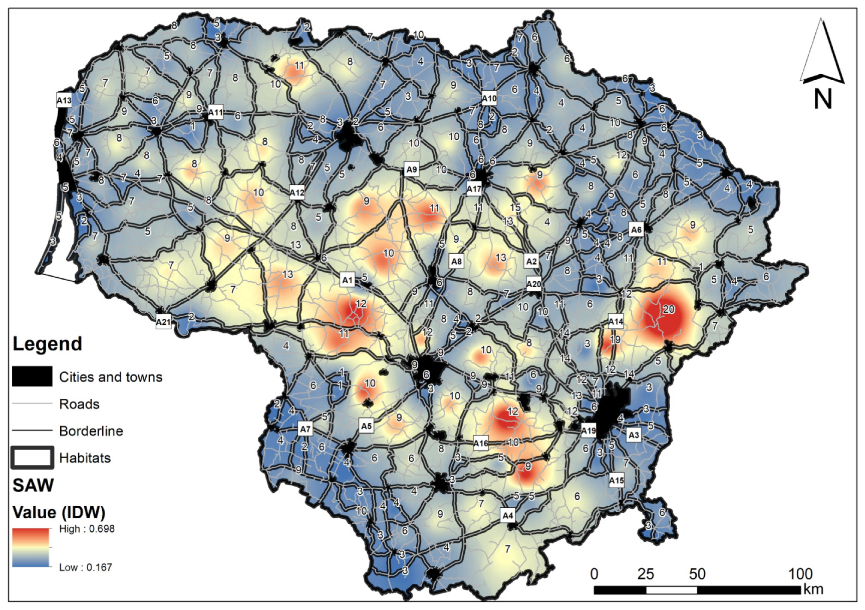
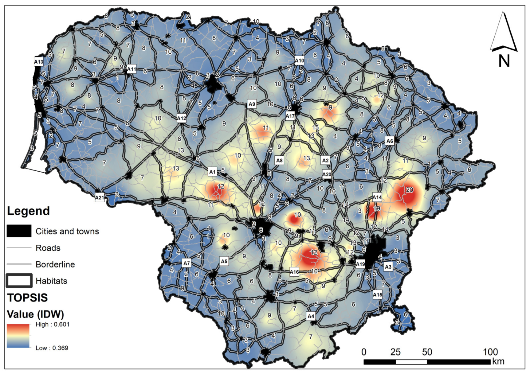
3.2. Criteria Weights, Habitat Ranks, Ecological Corridors, and Movement Patterns
3.3. Relationship between Habitat Ranks, Species Richness, and Land Cover Classes
4. Discussion
4.1. Habitat Risk Severity to Drivers
4.2. Habitat Attractiveness to Mammals
4.3. Multi-Objective Mitigation Measures
5. Conclusions
- Habitats were characterised by connectivity, land cover, roadkill, roadkill cluster, and mammal species and ranked using multiple criteria for the identification of habitat risk severity to drivers and attractiveness to wildlife;
- Despite the potential limitations of the scope of the roadkill data, our habitat ranking suggests that this procedure can provide information on habitats, habitat locations, species richness, habitat risk severity to drivers, and attractiveness to wildlife;
- Strong relationships were identified and discussed between the habitat patch ranks, five (out of 28) land cover classes, and eight (out of 28) species (97% of all mammal road kills);
- This methodology facilitates decision-making on the habitats that must be prioritized to preserve wildlife in the vicinity of roads that are prone to MVCs. It is also suitable for the planning of multi-objective mitigation measures to improve road security in a dynamic environment.
Author Contributions
Funding
Institutional Review Board Statement
Data Availability Statement
Acknowledgments
Conflicts of Interest
Appendix A

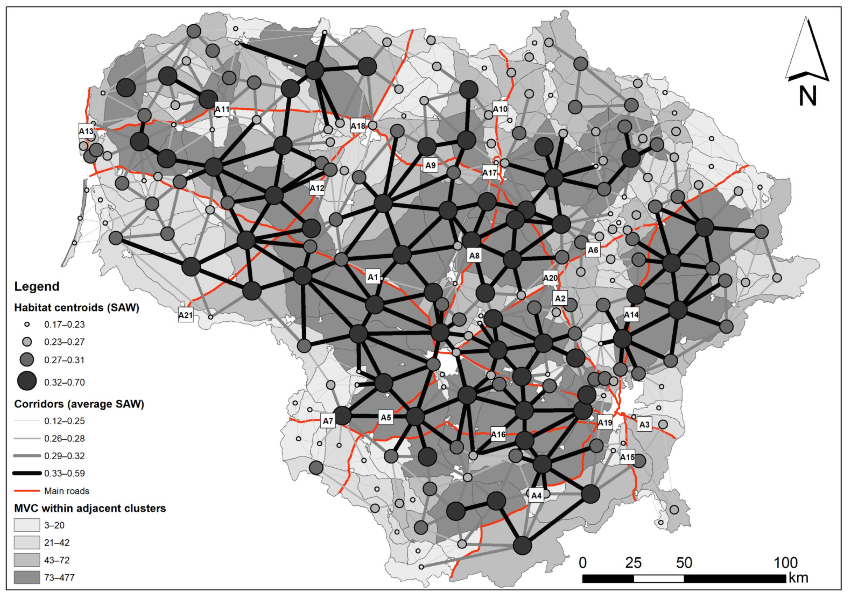
| Unique Identification Number of Habitat (Figure 3) | Total Area of (ha): | Number of Adjacent: | Total Length of Adjacent (km): | Number of Collisions (MVC) within Adjacent Clusters | Average Strength of Adjacent Clusters (KDE+) | ||||
|---|---|---|---|---|---|---|---|---|---|
| Habitat Patch | Adjacent Habitat Patches | Clusters | Corridors | Corridors | Pathways to Clusters | Clusters | |||
| 6 | 139,650.90 | 200,454.05 | 10 | 6 | 202.50 | 214.45 | 3.60 | 45 | 0.4081 |
| 12 | 32,970.44 | 177,828.03 | 3 | 4 | 102.88 | 37.15 | 0.59 | 6 | 0.3919 |
| 15 | 9886.41 | 82,018.06 | 5 | 4 | 55.59 | 30.78 | 0.84 | 11 | 0.3530 |
| 25 | 20,544.02 | 293,639.62 | 7 | 6 | 140.00 | 53.80 | 1.64 | 18 | 0.3777 |
| 27 | 49,493.57 | 105,316.53 | 25 | 5 | 90.43 | 301.53 | 7.06 | 107 | 0.4034 |
| 29 | 7746.70 | 110,394.31 | 9 | 5 | 76.99 | 49.82 | 2.67 | 37 | 0.4663 |
| 30 | 20,756.90 | 133,555.22 | 12 | 7 | 114.14 | 95.74 | 3.84 | 56 | 0.3973 |
| 42 | 56,222.02 | 45,595.47 | 19 | 3 | 81.38 | 578.92 | 3.64 | 44 | 0.3999 |
| 49 | 8263.08 | 78,347.16 | 3 | 2 | 41.45 | 33.45 | 0.54 | 6 | 0.3491 |
| 65 | 86,540.34 | 287,351.74 | 12 | 6 | 168.75 | 267.29 | 3.67 | 45 | 0.4512 |
| 69 | 13,269.35 | 123,512.66 | 11 | 6 | 85.77 | 99.30 | 3.26 | 43 | 0.4903 |
| 81 | 40,881.40 | 237,462.40 | 26 | 6 | 133.16 | 297.33 | 6.90 | 113 | 0.3696 |
| 84 | 10,394.58 | 88,278.91 | 5 | 4 | 55.15 | 29.58 | 2.31 | 34 | 0.3914 |
| 105 | 22,220.59 | 153,376.31 | 17 | 6 | 106.67 | 142.58 | 4.79 | 64 | 0.4851 |
| 107 | 6097.13 | 295,799.24 | 8 | 5 | 86.22 | 38.80 | 1.81 | 26 | 0.3532 |
| 109 | 26,971.83 | 141,639.80 | 11 | 6 | 135.03 | 125.33 | 2.40 | 33 | 0.4293 |
| 114 | 13,420.71 | 313,371.47 | 6 | 4 | 72.12 | 40.04 | 1.26 | 20 | 0.4183 |
| 139 | 22,125.14 | 183,833.68 | 16 | 6 | 137.47 | 143.62 | 4.36 | 63 | 0.4556 |
| 145 | 81,083.09 | 199,083.28 | 54 | 7 | 147.61 | 1330.48 | 14.44 | 230 | 0.4003 |
| 149 | 913.63 | 202,816.14 | 8 | 7 | 130.44 | 15.42 | 2.82 | 48 | 0.4873 |
| 159 | 26,302.43 | 156,552.24 | 19 | 5 | 91.64 | 177.86 | 4.92 | 74 | 0.3987 |
| 163 | 19,150.25 | 116,087.17 | 3 | 5 | 91.54 | 22.00 | 0.49 | 8 | 0.3044 |
| 170 | 39,785.55 | 139,555.23 | 26 | 5 | 91.86 | 288.08 | 6.47 | 77 | 0.4501 |
| 182 | 10,805.79 | 135,726.79 | 8 | 4 | 52.26 | 49.21 | 2.00 | 20 | 0.4316 |
| 185 | 20,763.14 | 172,284.99 | 17 | 6 | 113.47 | 240.50 | 3.85 | 49 | 0.3928 |
| 192 | 29,897.38 | 65,613.76 | 10 | 4 | 54.50 | 103.37 | 1.90 | 26 | 0.3510 |
| 194 | 3369.45 | 237,614.49 | 4 | 6 | 130.76 | 9.11 | 1.46 | 23 | 0.5280 |
| 208 | 6795.19 | 69,431.17 | 5 | 5 | 66.65 | 17.48 | 1.75 | 27 | 0.5321 |
| 210 | 11,376.97 | 107,910.32 | 7 | 5 | 67.54 | 53.89 | 1.56 | 16 | 0.4786 |
| 212 | 28,632.79 | 59,050.92 | 8 | 4 | 60.40 | 78.05 | 1.80 | 20 | 0.4757 |
| 214 | 32,032.08 | 190,092.71 | 6 | 8 | 175.94 | 61.15 | 1.31 | 17 | 0.4390 |
| 218 | 39,940.29 | 212,569.11 | 35 | 5 | 96.67 | 532.34 | 10.46 | 177 | 0.4332 |
| 250 | 15,207.25 | 131,842.62 | 11 | 6 | 127.65 | 76.62 | 2.11 | 27 | 0.4054 |
| 255 | 58,086.51 | 285,182.80 | 25 | 8 | 202.54 | 375.49 | 5.85 | 105 | 0.4294 |
| 267 | 20,266.12 | 202,654.73 | 18 | 6 | 117.49 | 141.77 | 5.35 | 76 | 0.4140 |
| 294 | 8114.69 | 332,292.67 | 12 | 9 | 199.44 | 65.72 | 2.81 | 32 | 0.4470 |
| 313 | 54,397.11 | 197,333.56 | 26 | 9 | 194.20 | 390.66 | 7.77 | 149 | 0.3597 |
| 349 | 1026.87 | 37,640.64 | 2 | 3 | 42.03 | 4.42 | 0.42 | 5 | 0.4798 |
| 363 | 14,293.62 | 96,397.55 | 4 | 5 | 72.93 | 28.90 | 0.77 | 9 | 0.4270 |
| 371 | 15,638.20 | 54,135.88 | 7 | 4 | 51.56 | 37.97 | 1.54 | 16 | 0.4737 |
| 388 | 41,864.59 | 79,652.04 | 8 | 6 | 103.05 | 97.75 | 1.59 | 17 | 0.4521 |
| 407 | 16,006.40 | 41,733.83 | 24 | 5 | 62.46 | 182.59 | 7.09 | 127 | 0.4176 |
| 427 | 6408.49 | 84,791.01 | 2 | 3 | 45.25 | 10.00 | 0.42 | 4 | 0.4930 |
| 430 | 53,447.47 | 140,843.94 | 29 | 8 | 153.38 | 541.35 | 7.49 | 101 | 0.4734 |
| 439 | 5374.78 | 67,230.93 | 6 | 6 | 71.85 | 22.70 | 1.49 | 25 | 0.3304 |
| 450 | 406.03 | 161,433.60 | 9 | 6 | 95.49 | 21.48 | 2.35 | 54 | 0.4300 |
| 455 | 40,050.24 | 279,808.91 | 8 | 5 | 152.33 | 97.57 | 2.34 | 23 | 0.4668 |
| 460 | 4956.26 | 159,646.28 | 9 | 4 | 52.22 | 34.46 | 3.78 | 72 | 0.3962 |
| 472 | 7866.55 | 87,828.86 | 11 | 6 | 90.31 | 70.93 | 2.88 | 68 | 0.4175 |
| 474 | 8684.84 | 15,464.01 | 12 | 4 | 32.74 | 66.13 | 2.91 | 46 | 0.3780 |
| 484 | 8547.01 | 69,712.63 | 14 | 5 | 54.50 | 75.37 | 3.92 | 95 | 0.3897 |
| 486 | 6332.88 | 173,689.79 | 2 | 4 | 49.39 | 9.39 | 0.38 | 4 | 0.4377 |
| 493 | 30,035.21 | 55,487.94 | 8 | 4 | 55.55 | 70.16 | 2.06 | 27 | 0.4608 |
| 496 | 2851.82 | 126,623.42 | 8 | 5 | 69.66 | 27.55 | 2.50 | 54 | 0.3609 |
| 501 | 4449.84 | 114,707.35 | 5 | 4 | 50.59 | 14.77 | 1.14 | 14 | 0.4892 |
| 502 | 59,532.25 | 72,106.47 | 34 | 7 | 120.92 | 448.42 | 12.26 | 233 | 0.4272 |
| 505 | 7099.46 | 232,115.55 | 14 | 7 | 107.84 | 67.28 | 4.60 | 95 | 0.4451 |
| 518 | 15,350.47 | 130,369.46 | 13 | 7 | 111.52 | 98.47 | 4.56 | 72 | 0.3834 |
| 526 | 551.67 | 65,675.38 | 7 | 5 | 55.70 | 9.24 | 1.93 | 42 | 0.4503 |
| 530 | 1671.02 | 54,468.27 | 11 | 5 | 44.23 | 37.72 | 3.16 | 78 | 0.4152 |
| 533 | 4452.12 | 271,067.83 | 3 | 5 | 83.56 | 15.29 | 0.59 | 6 | 0.4561 |
| 542 | 842.71 | 255,407.87 | 4 | 6 | 127.53 | 8.53 | 1.12 | 23 | 0.4925 |
| 547 | 16,775.94 | 239,527.33 | 10 | 5 | 114.00 | 71.23 | 4.50 | 66 | 0.4707 |
| 577 | 148,761.11 | 139,830.71 | 64 | 7 | 180.59 | 1623.02 | 19.96 | 477 | 0.4834 |
| 587 | 31,309.97 | 91,225.40 | 8 | 7 | 108.87 | 79.98 | 1.73 | 19 | 0.4083 |
| 588 | 16,143.01 | 250,902.96 | 30 | 7 | 143.51 | 265.72 | 8.98 | 294 | 0.4930 |
| 593 | 5028.73 | 167,525.08 | 11 | 6 | 89.96 | 78.10 | 3.64 | 71 | 0.3318 |
| 594 | 638.35 | 132,279.96 | 4 | 5 | 85.21 | 7.39 | 1.84 | 32 | 0.3771 |
| 608 | 27,848.17 | 73,135.06 | 17 | 7 | 89.06 | 181.17 | 3.89 | 50 | 0.4399 |
| 642 | 120,160.25 | 163,452.54 | 42 | 6 | 159.99 | 1052.79 | 14.11 | 291 | 0.4690 |
| 656 | 6828.41 | 97,816.57 | 12 | 5 | 57.81 | 87.08 | 2.89 | 36 | 0.4691 |
| 661 | 36,721.46 | 258,703.50 | 14 | 5 | 138.30 | 254.92 | 3.38 | 44 | 0.4192 |
| 668 | 22,672.16 | 259,011.55 | 5 | 3 | 111.59 | 150.84 | 1.22 | 12 | 0.4795 |
| 674 | 8670.38 | 246,371.53 | 22 | 8 | 163.20 | 125.72 | 7.85 | 178 | 0.5224 |
| 688 | 43,933.50 | 109,036.29 | 16 | 7 | 123.69 | 203.36 | 3.64 | 44 | 0.3900 |
| 694 | 113.52 | 191,806.33 | 2 | 7 | 108.51 | 1.71 | 0.62 | 8 | 0.4044 |
| 697 | 1127.42 | 97,322.29 | 4 | 5 | 45.04 | 8.33 | 0.92 | 9 | 0.4802 |
| 714 | 2999.93 | 64,663.82 | 5 | 4 | 32.25 | 15.65 | 0.96 | 11 | 0.3500 |
| 721 | 35,574.69 | 160,770.09 | 18 | 7 | 124.19 | 187.91 | 4.90 | 66 | 0.4099 |
| 723 | 14,918.98 | 51,106.71 | 16 | 4 | 44.41 | 132.84 | 4.19 | 92 | 0.4803 |
| 728 | 29,942.96 | 94,841.87 | 19 | 6 | 105.29 | 241.89 | 4.83 | 82 | 0.4239 |
| 745 | 59,675.07 | 253,380.91 | 11 | 6 | 180.15 | 176.09 | 2.19 | 24 | 0.4566 |
| 746 | 11,572.92 | 276,983.34 | 15 | 7 | 144.76 | 109.63 | 4.22 | 68 | 0.3886 |
| 767 | 21,779.78 | 197,364.85 | 15 | 4 | 68.84 | 129.11 | 3.79 | 54 | 0.4355 |
| 768 | 73,317.38 | 373,589.09 | 20 | 7 | 206.77 | 283.63 | 5.23 | 103 | 0.3799 |
| 770 | 102,723.38 | 298,359.55 | 16 | 6 | 178.11 | 326.31 | 3.46 | 41 | 0.4190 |
| 789 | 123,084.90 | 189,787.84 | 33 | 6 | 155.53 | 726.81 | 9.52 | 130 | 0.4333 |
| 791 | 96,613.09 | 284,751.11 | 18 | 5 | 144.74 | 297.36 | 4.47 | 55 | 0.4172 |
| 795 | 1704.22 | 289,397.87 | 6 | 6 | 115.97 | 22.12 | 1.51 | 49 | 0.4971 |
| 805 | 9181.59 | 163,837.55 | 11 | 5 | 90.35 | 75.59 | 2.35 | 37 | 0.4059 |
| 813 | 15,330.96 | 122,295.05 | 11 | 6 | 96.95 | 82.02 | 3.14 | 66 | 0.3218 |
| 814 | 60,899.32 | 106,904.68 | 13 | 3 | 74.10 | 177.67 | 3.04 | 31 | 0.4411 |
| 817 | 10,487.36 | 180,491.33 | 8 | 5 | 93.20 | 55.64 | 1.79 | 26 | 0.4502 |
| 827 | 8152.71 | 103,750.13 | 7 | 4 | 49.23 | 39.81 | 2.09 | 40 | 0.3644 |
| 839 | 3269.34 | 257,878.86 | 5 | 4 | 77.02 | 29.51 | 1.21 | 19 | 0.3707 |
| 857 | 12,897.86 | 111,902.63 | 8 | 5 | 69.55 | 53.26 | 1.82 | 24 | 0.3679 |
| 868 | 3015.25 | 121,799.88 | 4 | 6 | 98.02 | 15.75 | 0.86 | 17 | 0.3900 |
| 878 | 22,351.00 | 90,552.99 | 16 | 5 | 74.46 | 154.28 | 4.22 | 103 | 0.4157 |
| 881 | 89,590.76 | 150,862.11 | 29 | 6 | 135.03 | 500.15 | 7.93 | 141 | 0.4503 |
| 912 | 26,621.53 | 110,432.37 | 12 | 6 | 95.02 | 108.57 | 3.26 | 49 | 0.3266 |
| 913 | 81,476.51 | 281,052.45 | 36 | 6 | 139.18 | 658.06 | 11.69 | 159 | 0.4182 |
| 924 | 45,311.39 | 304,598.21 | 20 | 7 | 158.74 | 265.97 | 5.37 | 120 | 0.4233 |
| 945 | 1394.92 | 384,991.16 | 2 | 6 | 124.12 | 3.54 | 0.48 | 5 | 0.4912 |
| 962 | 17,292.37 | 103,458.26 | 8 | 7 | 98.88 | 78.87 | 2.26 | 31 | 0.4659 |
| 967 | 98,955.66 | 175,763.59 | 24 | 7 | 164.13 | 413.74 | 6.13 | 94 | 0.4509 |
| 988 | 3060.79 | 436,613.07 | 5 | 7 | 170.72 | 21.79 | 1.49 | 23 | 0.4690 |
| 1028 | 28,199.78 | 161,276.22 | 20 | 6 | 115.64 | 290.72 | 6.78 | 140 | 0.3881 |
| 1034 | 45,987.96 | 427,134.53 | 16 | 8 | 222.17 | 193.22 | 4.25 | 58 | 0.3733 |
| 1037 | 4155.04 | 181,101.39 | 16 | 5 | 90.50 | 99.08 | 4.74 | 89 | 0.3982 |
| 1041 | 59,317.61 | 243,963.67 | 12 | 5 | 112.18 | 226.55 | 2.34 | 25 | 0.3946 |
| 1067 | 8615.61 | 229,667.24 | 7 | 7 | 144.12 | 35.62 | 2.99 | 51 | 0.3589 |
| 1076 | 12,362.06 | 109,332.11 | 19 | 5 | 65.93 | 135.30 | 6.33 | 107 | 0.3906 |
| 1086 | 26,082.13 | 205,227.06 | 13 | 7 | 148.29 | 114.91 | 3.02 | 35 | 0.4076 |
| 1097 | 13,347.14 | 126,268.91 | 13 | 7 | 95.26 | 99.40 | 3.76 | 59 | 0.4014 |
| 1098 | 32,653.14 | 159,838.18 | 19 | 5 | 109.33 | 197.80 | 6.16 | 78 | 0.4310 |
| 1107 | 59,695.86 | 212,908.34 | 13 | 6 | 153.40 | 189.37 | 3.06 | 44 | 0.4832 |
| 1114 | 77,091.89 | 289,196.36 | 22 | 7 | 190.06 | 350.43 | 6.37 | 83 | 0.4176 |
| 1115 | 86,544.04 | 356,520.16 | 26 | 8 | 244.87 | 499.88 | 6.05 | 72 | 0.4151 |
| 1116 | 787.12 | 38,519.26 | 3 | 4 | 26.58 | 5.12 | 0.55 | 8 | 0.3514 |
| 1126 | 26,486.94 | 209,006.42 | 15 | 4 | 71.82 | 230.05 | 3.16 | 44 | 0.3920 |
| 1133 | 22,831.99 | 210,541.11 | 14 | 5 | 89.80 | 141.13 | 5.17 | 112 | 0.3376 |
| 1134 | 10,165.22 | 88,243.02 | 10 | 5 | 61.36 | 52.30 | 2.80 | 38 | 0.4820 |
| 1156 | 46,637.37 | 282,819.38 | 16 | 9 | 195.23 | 206.97 | 3.83 | 57 | 0.3521 |
| 1163 | 14,093.66 | 316,790.63 | 6 | 6 | 127.59 | 38.48 | 1.23 | 17 | 0.2998 |
| 1169 | 5713.44 | 50,558.89 | 7 | 6 | 52.52 | 33.05 | 1.86 | 25 | 0.5095 |
| 1183 | 2729.25 | 37,035.79 | 2 | 5 | 38.27 | 4.85 | 0.39 | 4 | 0.4581 |
| 1186 | 28,020.86 | 254,445.78 | 19 | 7 | 142.02 | 176.61 | 4.62 | 94 | 0.4864 |
| 1190 | 3864.25 | 247,170.44 | 7 | 5 | 97.64 | 75.05 | 1.97 | 25 | 0.4169 |
| 1226 | 57,029.73 | 166,243.04 | 10 | 7 | 127.21 | 199.43 | 2.83 | 30 | 0.4426 |
| 1229 | 18,092.33 | 182,645.42 | 13 | 6 | 110.63 | 87.64 | 5.95 | 92 | 0.4375 |
| 1230 | 6752.07 | 156,443.64 | 2 | 6 | 97.55 | 12.95 | 0.37 | 4 | 0.4233 |
| 1235 | 8685.78 | 33,343.23 | 7 | 4 | 46.77 | 36.13 | 2.12 | 20 | 0.4726 |
| 1240 | 6237.78 | 105,562.83 | 6 | 6 | 74.03 | 26.95 | 2.04 | 34 | 0.4520 |
| 1245 | 32,749.54 | 171,518.38 | 16 | 7 | 121.81 | 174.41 | 4.65 | 83 | 0.3271 |
| 1250 | 15,274.28 | 176,484.33 | 16 | 5 | 80.88 | 131.18 | 4.66 | 61 | 0.4613 |
| 1281 | 33,658.14 | 88,145.48 | 14 | 5 | 77.94 | 163.87 | 3.00 | 34 | 0.4529 |
| 1283 | 7568.01 | 131,088.86 | 5 | 7 | 95.31 | 26.06 | 1.30 | 15 | 0.3860 |
| 1289 | 16,729.43 | 42,515.68 | 12 | 5 | 50.80 | 91.01 | 3.51 | 52 | 0.3805 |
| 1294 | 24,681.00 | 211,432.77 | 4 | 5 | 96.24 | 35.94 | 1.19 | 17 | 0.4695 |
| 1295 | 18,084.15 | 223,680.12 | 10 | 7 | 127.52 | 65.36 | 2.81 | 32 | 0.4252 |
| 1306 | 72,066.64 | 151,755.00 | 37 | 7 | 154.21 | 669.36 | 11.31 | 217 | 0.3624 |
| 1307 | 11,322.00 | 185,508.44 | 7 | 5 | 81.89 | 46.77 | 1.77 | 26 | 0.4137 |
| 1346 | 26,494.20 | 100,497.63 | 8 | 6 | 93.29 | 84.91 | 2.00 | 34 | 0.3864 |
| 1358 | 3699.64 | 20,747.85 | 14 | 4 | 52.69 | 142.23 | 3.94 | 84 | 0.3620 |
| 1361 | 424.04 | 34,852.89 | 6 | 3 | 40.20 | 27.61 | 1.99 | 46 | 0.4280 |
| 1397 | 670.21 | 67,738.18 | 3 | 3 | 54.17 | 4.27 | 0.73 | 13 | 0.3525 |
| 1399 | 71,832.91 | 289,533.30 | 28 | 8 | 199.92 | 522.36 | 6.20 | 82 | 0.3709 |
| 1406 | 10,441.83 | 236,626.73 | 10 | 6 | 106.40 | 64.25 | 3.04 | 35 | 0.4599 |
| 1421 | 6521.17 | 199,715.34 | 17 | 6 | 111.34 | 95.68 | 4.06 | 55 | 0.3914 |
| 1424 | 7075.41 | 127,018.38 | 4 | 4 | 49.50 | 24.32 | 0.80 | 16 | 0.4225 |
| 1437 | 21,446.06 | 278,307.57 | 11 | 7 | 153.66 | 100.68 | 3.10 | 53 | 0.3250 |
| 1444 | 24,969.18 | 113,672.42 | 4 | 5 | 87.69 | 41.17 | 1.48 | 19 | 0.4627 |
| 1452 | 33,839.26 | 150,121.36 | 21 | 6 | 105.84 | 208.66 | 6.27 | 84 | 0.4571 |
| 1462 | 15,010.46 | 189,536.41 | 19 | 4 | 65.83 | 134.36 | 4.49 | 63 | 0.3714 |
| 1475 | 14,808.02 | 82,476.01 | 7 | 6 | 76.88 | 55.63 | 1.97 | 34 | 0.5179 |
| 1478 | 1949.18 | 81,757.01 | 6 | 4 | 53.73 | 18.19 | 1.79 | 32 | 0.3442 |
| 1492 | 40,178.40 | 217,814.35 | 17 | 6 | 131.45 | 187.58 | 3.75 | 63 | 0.3973 |
| 1496 | 1408.69 | 140,511.54 | 9 | 5 | 77.56 | 22.37 | 2.23 | 42 | 0.4113 |
| 1505 | 21,628.32 | 139,095.96 | 11 | 7 | 116.70 | 91.87 | 2.92 | 30 | 0.4774 |
| 1507 | 977.68 | 175,298.34 | 5 | 6 | 104.25 | 7.71 | 1.67 | 38 | 0.4843 |
| 1518 | 28,064.51 | 114,924.57 | 22 | 7 | 107.51 | 242.41 | 7.62 | 146 | 0.3569 |
| 1519 | 90,703.78 | 241,999.71 | 22 | 7 | 174.59 | 389.71 | 4.65 | 63 | 0.3948 |
| 1524 | 279.17 | 22,245.26 | 3 | 3 | 18.66 | 5.40 | 0.72 | 12 | 0.4726 |
| 1532 | 49,396.90 | 164,132.83 | 21 | 7 | 137.65 | 298.00 | 5.93 | 94 | 0.3801 |
| 1533 | 33,873.78 | 110,225.07 | 25 | 4 | 62.59 | 284.54 | 6.22 | 104 | 0.3429 |
| 1534 | 9535.38 | 101,188.48 | 13 | 5 | 66.96 | 84.17 | 4.68 | 97 | 0.4054 |
| 1557 | 9936.36 | 98,767.85 | 9 | 6 | 77.03 | 55.41 | 2.47 | 40 | 0.4222 |
| 1558 | 18,251.82 | 109,634.35 | 13 | 6 | 100.03 | 106.30 | 4.69 | 91 | 0.4045 |
| 1560 | 7908.16 | 214,037.46 | 14 | 7 | 128.26 | 80.78 | 3.19 | 36 | 0.4075 |
| 1562 | 3397.56 | 13,000.93 | 5 | 4 | 30.57 | 18.12 | 1.39 | 27 | 0.5100 |
| 1568 | 4039.68 | 24,080.89 | 6 | 4 | 23.87 | 21.96 | 1.77 | 26 | 0.5915 |
| 1569 | 39,551.03 | 86,889.66 | 4 | 5 | 108.00 | 38.76 | 1.43 | 18 | 0.4485 |
| 1578 | 5596.14 | 25,331.20 | 9 | 4 | 31.73 | 40.50 | 2.86 | 51 | 0.5361 |
| 1594 | 47,007.60 | 103,575.45 | 20 | 8 | 150.55 | 261.14 | 6.32 | 103 | 0.4576 |
| 1597 | 29,272.60 | 100,781.16 | 19 | 7 | 118.82 | 203.48 | 4.24 | 66 | 0.3757 |
| 1601 | 11,606.92 | 91,238.03 | 10 | 5 | 67.79 | 71.71 | 3.18 | 55 | 0.4186 |
| 1608 | 20,713.92 | 85,718.96 | 16 | 5 | 72.09 | 150.38 | 6.10 | 108 | 0.3762 |
| 1610 | 22,556.62 | 173,460.63 | 18 | 5 | 103.06 | 149.97 | 3.94 | 62 | 0.4065 |
| 1633 | 7985.15 | 104,340.98 | 13 | 6 | 83.77 | 67.19 | 3.44 | 71 | 0.3290 |
| 1638 | 12,344.12 | 212,857.39 | 10 | 5 | 85.90 | 69.94 | 2.35 | 36 | 0.3649 |
| 1639 | 1687.87 | 173,026.58 | 3 | 5 | 102.57 | 9.39 | 0.76 | 10 | 0.2541 |
| 1647 | 9878.36 | 95,779.10 | 20 | 5 | 60.78 | 112.47 | 5.33 | 84 | 0.4204 |
| 1653 | 19,429.28 | 152,497.77 | 5 | 6 | 110.43 | 44.90 | 1.07 | 11 | 0.5182 |
| 1654 | 896.17 | 161,786.45 | 6 | 6 | 100.72 | 9.37 | 1.29 | 21 | 0.3603 |
| 1671 | 6958.72 | 128,202.48 | 14 | 5 | 77.31 | 96.41 | 3.37 | 58 | 0.3581 |
| 1675 | 7633.48 | 121,198.20 | 10 | 5 | 68.96 | 62.58 | 2.07 | 34 | 0.3651 |
| 1679 | 5533.32 | 275,379.01 | 2 | 5 | 93.62 | 9.75 | 0.39 | 4 | 0.4524 |
| 1681 | 48,186.10 | 122,791.45 | 20 | 5 | 92.73 | 256.60 | 5.16 | 68 | 0.4215 |
| 1700 | 20,889.61 | 189,438.39 | 17 | 7 | 131.67 | 194.62 | 4.63 | 68 | 0.3667 |
| 1706 | 3085.94 | 111,060.99 | 3 | 6 | 101.86 | 7.74 | 0.81 | 14 | 0.4478 |
| 1715 | 12,195.17 | 94,176.12 | 7 | 5 | 84.10 | 52.02 | 2.35 | 45 | 0.3747 |
| 1731 | 15,219.57 | 165,458.85 | 10 | 7 | 96.29 | 76.21 | 2.24 | 27 | 0.4569 |
| 1738 | 55,927.96 | 116,427.39 | 28 | 4 | 92.87 | 387.47 | 8.44 | 99 | 0.3379 |
| 1745 | 30,237.24 | 209,558.57 | 7 | 6 | 117.77 | 70.76 | 1.84 | 21 | 0.4572 |
| 1748 | 17,446.66 | 279,990.97 | 6 | 6 | 131.88 | 45.34 | 1.30 | 19 | 0.3747 |
| 1749 | 19,096.63 | 87,371.87 | 14 | 4 | 56.83 | 108.10 | 2.92 | 37 | 0.3756 |
| 1764 | 30,762.74 | 78,861.47 | 17 | 6 | 94.85 | 175.03 | 4.13 | 57 | 0.3799 |
| 1769 | 6344.60 | 85,765.72 | 7 | 5 | 54.05 | 40.60 | 1.50 | 16 | 0.4538 |
| 1777 | 21,882.10 | 201,834.33 | 12 | 8 | 160.72 | 97.02 | 4.22 | 55 | 0.4025 |
| 1778 | 19,362.06 | 112,017.20 | 16 | 4 | 104.46 | 212.13 | 4.60 | 57 | 0.2977 |
| 1782 | 10,826.89 | 120,203.69 | 10 | 5 | 64.05 | 59.33 | 2.99 | 46 | 0.4271 |
| 1790 | 4967.14 | 132,758.39 | 4 | 6 | 92.82 | 17.89 | 0.80 | 12 | 0.3525 |
| 1794 | 39,864.90 | 284,582.45 | 11 | 6 | 146.02 | 156.82 | 2.41 | 32 | 0.4017 |
| 1798 | 51,201.38 | 85,322.04 | 22 | 5 | 93.40 | 317.22 | 5.45 | 68 | 0.4150 |
| 1812 | 27,755.98 | 164,965.06 | 6 | 6 | 113.93 | 64.07 | 1.33 | 17 | 0.3973 |
| 1816 | 49,558.70 | 140,839.59 | 19 | 6 | 116.25 | 248.76 | 5.68 | 72 | 0.4426 |
| 1826 | 10,977.84 | 194,907.87 | 4 | 7 | 137.28 | 35.05 | 0.77 | 11 | 0.3532 |
| 1834 | 13,150.92 | 51,656.98 | 7 | 3 | 42.72 | 35.24 | 1.56 | 18 | 0.4388 |
| 1853 | 17,579.71 | 98,804.55 | 14 | 3 | 54.98 | 195.40 | 3.76 | 39 | 0.4100 |
| 1864 | 44,062.02 | 175,180.04 | 23 | 6 | 118.97 | 306.20 | 6.15 | 70 | 0.3894 |
| 1866 | 73,170.00 | 189,601.82 | 18 | 7 | 177.14 | 319.39 | 3.99 | 47 | 0.4651 |
| 1876 | 35,035.12 | 161,066.27 | 5 | 6 | 122.93 | 46.46 | 1.19 | 12 | 0.4917 |
| 1877 | 21,524.06 | 134,671.99 | 33 | 7 | 120.46 | 297.69 | 7.16 | 105 | 0.3517 |
| 1879 | 63,771.53 | 111,222.35 | 15 | 5 | 123.75 | 197.72 | 5.18 | 69 | 0.4853 |
| 1882 | 25,628.08 | 142,367.89 | 11 | 5 | 84.92 | 114.24 | 2.41 | 29 | 0.4335 |
| 1913 | 18,601.09 | 133,829.94 | 20 | 6 | 100.98 | 190.26 | 5.72 | 73 | 0.4415 |
| 1916 | 26,067.02 | 97,119.28 | 20 | 5 | 70.92 | 195.93 | 5.52 | 72 | 0.3984 |
| 1966 | 24,889.16 | 48,516.32 | 13 | 4 | 59.28 | 142.07 | 3.81 | 50 | 0.4004 |
| 1986 | 10,376.30 | 157,970.95 | 4 | 7 | 153.83 | 24.50 | 0.96 | 9 | 0.4402 |
| 2004 | 18,419.25 | 172,357.90 | 7 | 5 | 119.25 | 65.55 | 1.63 | 25 | 0.5463 |
| 2014 | 2410.14 | 105,994.53 | 1 | 6 | 93.61 | 3.55 | 0.35 | 3 | 0.4506 |
| 2037 | 24,718.80 | 63,830.67 | 10 | 3 | 64.44 | 216.47 | 2.25 | 36 | 0.4385 |
| 2038 | 16,391.90 | 25,383.04 | 12 | 3 | 42.24 | 127.44 | 3.04 | 40 | 0.3997 |
| 2052 | 32,113.69 | 189,372.89 | 17 | 6 | 172.21 | 198.68 | 4.09 | 53 | 0.3576 |
| 2055 | 12,596.60 | 93,551.41 | 11 | 4 | 64.24 | 81.57 | 3.93 | 47 | 0.5472 |
| 2060 | 2450.68 | 282,984.78 | 4 | 7 | 177.34 | 14.43 | 0.66 | 8 | 0.3172 |
| 2105 | 11,678.01 | 229,612.31 | 3 | 5 | 164.37 | 28.76 | 0.90 | 9 | 0.5434 |
| 2106 | 18,325.75 | 72,309.40 | 8 | 4 | 87.07 | 68.23 | 1.63 | 19 | 0.4210 |
| 2224 | 513.57 | 155,393.82 | 3 | 5 | 61.12 | 5.00 | 0.61 | 10 | 0.4559 |
| 2229 | 33,511.21 | 67,059.07 | 13 | 4 | 72.74 | 158.39 | 3.01 | 42 | 0.3636 |
| 2233 | 19,071.18 | 124,934.73 | 9 | 5 | 87.46 | 67.43 | 2.16 | 28 | 0.4049 |
| 2237 | 469.96 | 169,750.82 | 2 | 5 | 106.25 | 3.05 | 0.39 | 6 | 0.3960 |
| 2244 | 15,623.84 | 76,303.43 | 7 | 4 | 49.94 | 50.12 | 1.38 | 20 | 0.4367 |
| 2246 | 1381.02 | 59,689.66 | 3 | 3 | 28.55 | 10.64 | 0.67 | 10 | 0.3596 |
| 2247 | 4885.96 | 70,126.78 | 8 | 3 | 51.26 | 52.32 | 1.95 | 38 | 0.3126 |
| 2248 | 95,297.89 | 122,224.14 | 58 | 7 | 158.06 | 980.16 | 17.59 | 334 | 0.4143 |
| 2249 | 119,258.39 | 141,390.65 | 42 | 6 | 128.49 | 861.51 | 10.65 | 160 | 0.4427 |
| 2250 | 12,055.54 | 258,374.60 | 16 | 7 | 153.61 | 119.02 | 4.74 | 96 | 0.4157 |
| 2251 | 63,561.74 | 366,751.45 | 31 | 7 | 209.27 | 592.77 | 8.38 | 92 | 0.4794 |
| 2252 | 16,490.07 | 148,897.07 | 5 | 4 | 92.80 | 38.48 | 1.51 | 21 | 0.4779 |
| 2253 | 22,467.48 | 141,782.65 | 9 | 7 | 118.89 | 88.74 | 2.16 | 32 | 0.5217 |
| 2254 | 38,634.75 | 170,998.75 | 15 | 6 | 130.44 | 223.51 | 3.45 | 41 | 0.4515 |
| 2255 | 117,246.63 | 145,041.02 | 35 | 6 | 159.50 | 897.39 | 8.29 | 100 | 0.4424 |
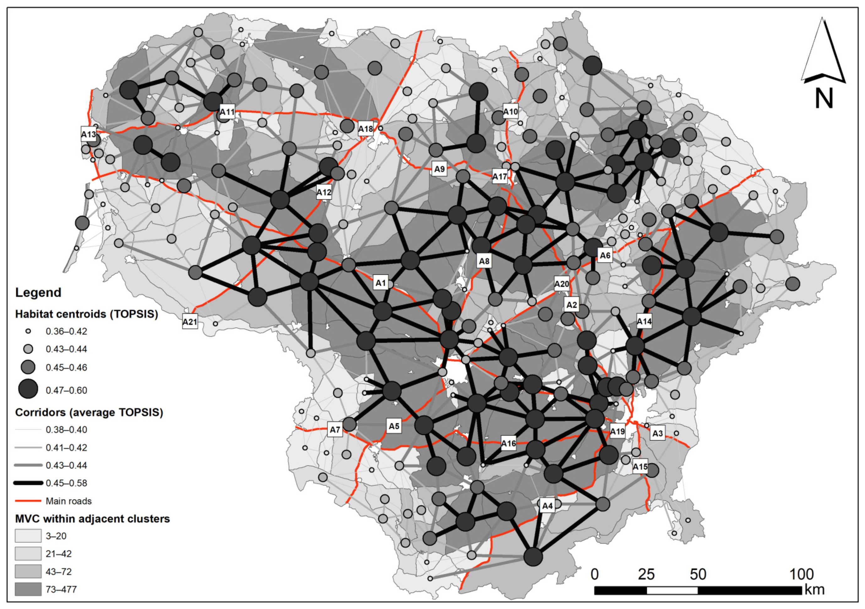
| Unique Identification Number of Habitat (Figure 3) | Ranks | Species | ||
|---|---|---|---|---|
| SAW | TOPSIS | Count | Latin Names | |
| 6 | 0.3508 | 0.4690 | 7 | M. meles, V. vulpes, E. concolor, N. procyonoides, A. alces, S. scrofa, C. capreolus |
| 12 | 0.2064 | 0.4166 | 3 | L. europaeus, S. scrofa, C. capreolus |
| 15 | 0.1856 | 0.4128 | 3 | A. alces, S. scrofa, C. capreolus |
| 25 | 0.2542 | 0.4239 | 4 | L. europaeus, V. vulpes, S. scrofa, C. capreolus |
| 27 | 0.3329 | 0.4683 | 9 | C. fiber, M. meles, M. putorius, C. elaphus, L. europaeus, V. vulpes, A. alces, S. scrofa, C. capreolus |
| 29 | 0.2264 | 0.4241 | 3 | A. alces, S. scrofa, C. capreolus |
| 30 | 0.2705 | 0.4363 | 6 | C. fiber, L. europaeus, E. concolor, A. alces, S. scrofa, C. capreolus |
| 42 | 0.2498 | 0.3686 | 6 | L. europaeus, V. vulpes, E. concolor, A. alces, S. scrofa, C. capreolus |
| 49 | 0.1689 | 0.4089 | 3 | A. alces, S. scrofa, C. capreolus |
| 65 | 0.3394 | 0.4414 | 6 | M. meles, L. europaeus, E. concolor, A. alces, S. scrofa, C. capreolus |
| 69 | 0.2547 | 0.4256 | 4 | C. elaphus, L. europaeus, S. scrofa, C. capreolus |
| 81 | 0.3468 | 0.4687 | 7 | M. meles, C. elaphus, V. vulpes, N. procyonoides, A. alces, S. scrofa, C. capreolus |
| 84 | 0.2112 | 0.4240 | 4 | E. concolor, A. alces, S. scrofa, C. capreolus |
| 105 | 0.2843 | 0.4396 | 4 | M. putorius, A. alces, S. scrofa, C. capreolus |
| 107 | 0.2503 | 0.4290 | 5 | V. vulpes, E. concolor, A. alces, S. scrofa, C. capreolus |
| 109 | 0.2691 | 0.4238 | 9 | R. norvegicus, M. putorius, Martes sp., L. europaeus, V. vulpes, E. concolor, N. procyonoides, A. alces, C. capreolus |
| 114 | 0.2558 | 0.4285 | 5 | V. vulpes, E. concolor, N. procyonoides, A. alces, C. capreolus |
| 139 | 0.2935 | 0.4391 | 7 | T. europaea, L. europaeus, V. vulpes, E. concolor, A. alces, S. scrofa, C. capreolus |
| 145 | 0.4994 | 0.4687 | 9 | C. elaphus, Martes sp., L. europaeus, V. vulpes, E. concolor, N. procyonoides, A. alces, S. scrofa, C. capreolus |
| 149 | 0.2646 | 0.4308 | 3 | L. europaeus, S. scrofa, C. capreolus |
| 159 | 0.2943 | 0.4477 | 8 | M. putorius, C. elaphus, Martes sp., L. europaeus, V. vulpes, A. alces, S. scrofa, C. capreolus |
| 163 | 0.1906 | 0.4136 | 4 | Martes sp., L. europaeus, V. vulpes, A. alces, |
| 170 | 0.3171 | 0.4493 | 6 | C. elaphus, L. europaeus, V. vulpes, A. alces, S. scrofa, C. capreolus |
| 182 | 0.2224 | 0.4208 | 3 | A. alces, S. scrofa, C. capreolus |
| 185 | 0.2693 | 0.4163 | 5 | C. elaphus, L. europaeus, A. alces, S. scrofa, C. capreolus |
| 192 | 0.2240 | 0.4220 | 6 | Martes sp., L. europaeus, V. vulpes, E. concolor, S. scrofa, C. capreolus |
| 194 | 0.2594 | 0.4205 | 3 | L. europaeus, S. scrofa, C. capreolus |
| 208 | 0.2332 | 0.4219 | 5 | T. europaea, E. concolor, A. alces, S. scrofa, C. capreolus |
| 210 | 0.2147 | 0.4146 | 2 | L. europaeus, C. capreolus |
| 212 | 0.2217 | 0.4195 | 4 | Martes sp., E. concolor, N. procyonoides, C. capreolus |
| 214 | 0.2705 | 0.4209 | 6 | L. europaeus, E. concolor, N. procyonoides, A. alces, S. scrofa, C. capreolus |
| 218 | 0.4073 | 0.4991 | 10 | M. putorius, C. elaphus, Martes sp., L. europaeus, V. vulpes, E. concolor, N. procyonoides, A. alces, S. scrofa, C. capreolus |
| 250 | 0.2342 | 0.4192 | 5 | L. europaeus, E. concolor, A. alces, S. scrofa, C. capreolus |
| 255 | 0.3937 | 0.4584 | 9 | C. elaphus, Martes sp., L. europaeus, V. vulpes, E. concolor, N. procyonoides, A. alces, S. scrofa, C. capreolus |
| 267 | 0.2992 | 0.4501 | 6 | Martes sp., E. concolor, N. procyonoides, A. alces, S. scrofa, C. capreolus |
| 294 | 0.3109 | 0.4310 | 5 | M. meles, L. europaeus, E. concolor, S. scrofa, C. capreolus |
| 313 | 0.3980 | 0.4812 | 10 | N. vison, M. putorius, Martes sp., L. europaeus, V. vulpes, E. concolor, N. procyonoides, A. alces, S. scrofa, C. capreolus |
| 349 | 0.2215 | 0.4103 | 4 | E. concolor, A. alces, S. scrofa, C. capreolus |
| 363 | 0.2070 | 0.4140 | 4 | L. europaeus, V. vulpes, E. concolor, C. capreolus |
| 371 | 0.2103 | 0.4179 | 3 | A. alces, S. scrofa, C. capreolus |
| 388 | 0.2463 | 0.4208 | 6 | M. meles, L. europaeus, V. vulpes, N. procyonoides, S. scrofa, C. capreolus |
| 407 | 0.3297 | 0.4810 | 13 | C. fiber, N. vison, S. vulgaris, M. martes, C. elaphus, Martes sp., L. europaeus, V. vulpes, E. concolor, N. procyonoides, A. alces, S. scrofa, C. capreolus |
| 427 | 0.2010 | 0.4105 | 2 | L. europaeus, C. capreolus |
| 430 | 0.3764 | 0.4324 | 8 | M. putorius, C. elaphus, V. vulpes, E. concolor, N. procyonoides, A. alces, S. scrofa, C. capreolus |
| 439 | 0.2127 | 0.4203 | 6 | L. europaeus, V. vulpes, N. procyonoides, A. alces, S. scrofa, C. capreolus |
| 450 | 0.2691 | 0.4374 | 9 | M. putorius, Martes sp., L. europaeus, V. vulpes, E. concolor, N. procyonoides, A. alces, S. scrofa, C. capreolus |
| 455 | 0.2716 | 0.4273 | 4 | D. dama, A. alces, S. scrofa, C. capreolus |
| 460 | 0.2725 | 0.4493 | 9 | M. putorius, Martes sp., L. europaeus, V. vulpes, E. concolor, N. procyonoides, A. alces, S. scrofa, C. capreolus |
| 472 | 0.2851 | 0.4444 | 14 | L. lutra, N. vison, S. vulgaris, M. martes, M. meles, M. putorius, C. elaphus, L. europaeus, V. vulpes, E. concolor, N. procyonoides, A. alces, S. scrofa, C. capreolus |
| 474 | 0.2440 | 0.4312 | 7 | C. elaphus, L. europaeus, V. vulpes, E. concolor, A. alces, S. scrofa, C. capreolus |
| 484 | 0.2880 | 0.4575 | 12 | C. fiber, M. martes, M. putorius, C. elaphus, Martes sp., L. europaeus, V. vulpes, E. concolor, N. procyonoides, A. alces, S. scrofa, C. capreolus |
| 486 | 0.2152 | 0.4131 | 1 | C. capreolus |
| 493 | 0.2208 | 0.4228 | 3 | A. alces, S. scrofa, C. capreolus |
| 496 | 0.2481 | 0.4365 | 9 | M. putorius, Martes sp., L. europaeus, V. vulpes, E. concolor, N. procyonoides, A. alces, S. scrofa, C. capreolus |
| 501 | 0.2209 | 0.4173 | 3 | A. alces, S. scrofa, C. capreolus |
| 502 | 0.4247 | 0.5521 | 10 | N. vison, M. putorius, Martes sp., L. europaeus, V. vulpes, E. concolor, N. procyonoides, A. alces, S. scrofa, C. capreolus |
| 505 | 0.3324 | 0.4649 | 11 | S. vulgaris, M. meles, M. putorius, Martes sp., L. europaeus, V. vulpes, E. concolor, N. procyonoides, A. alces, S. scrofa, C. capreolus |
| 518 | 0.3129 | 0.4537 | 14 | C. fiber, S. vulgaris, M. martes, M. meles, M. putorius, C. elaphus, Martes sp., L. europaeus, V. vulpes, E. concolor, N. procyonoides, A. alces, S. scrofa, C. capreolus |
| 526 | 0.2735 | 0.4355 | 12 | L. lutra, N. vison, S. vulgaris, M. martes, M. meles, M. putorius, V. vulpes, E. concolor, N. procyonoides, A. alces, S. scrofa, C. capreolus |
| 530 | 0.2765 | 0.4482 | 11 | C. fiber, M. martes, M. putorius, C. elaphus, Martes sp., V. vulpes, E. concolor, N. procyonoides, A. alces, S. scrofa, C. capreolus |
| 533 | 0.2278 | 0.4157 | 1 | C. capreolus |
| 542 | 0.2862 | 0.4264 | 9 | M. meles, Martes sp., L. europaeus, V. vulpes, E. concolor, N. procyonoides, A. alces, S. scrofa, C. capreolus |
| 547 | 0.2807 | 0.4453 | 5 | L. europaeus, N. procyonoides, A. alces, S. scrofa, C. capreolus |
| 577 | 0.6981 | 0.5850 | 20 | O. zibethicus, M. erminea, L. lutra, M. foina, T. europaea, C. fiber, N. vison, S. vulgaris, M. martes, M. meles, M. putorius, C. elaphus, Martes sp., L. europaeus, V. vulpes, E. concolor, N. procyonoides, A. alces, S. scrofa, C. capreolus |
| 587 | 0.2307 | 0.4174 | 3 | A. alces, S. scrofa, C. capreolus |
| 588 | 0.4762 | 0.5779 | 19 | O. zibethicus, M. erminea, L. lutra, M. foina, T. europaea, C. fiber, N. vison, S. vulgaris, M. martes, M. meles, M. putorius, Martes sp., L. europaeus, V. vulpes, E. concolor, N. procyonoides, A. alces, S. scrofa, C. capreolus |
| 593 | 0.2931 | 0.4495 | 14 | C. fiber, S. vulgaris, M. martes, M. meles, M. putorius, C. elaphus, Martes sp., L. europaeus, V. vulpes, E. concolor, N. procyonoides, A. alces, S. scrofa, C. capreolus |
| 594 | 0.2487 | 0.4269 | 9 | M. putorius, Martes sp., L. europaeus, V. vulpes, E. concolor, N. procyonoides, A. alces, S. scrofa, C. capreolus |
| 608 | 0.2888 | 0.4316 | 8 | Martes sp., L. europaeus, V. vulpes, E. concolor, N. procyonoides, A. alces, S. scrofa, C. capreolus |
| 642 | 0.5255 | 0.5489 | 12 | L. timidus, M. meles, M. putorius, C. elaphus, Martes sp., L. europaeus, V. vulpes, E. concolor, N. procyonoides, A. alces, S. scrofa, C. capreolus |
| 656 | 0.2457 | 0.4247 | 5 | Martes sp., L. europaeus, A. alces, S. scrofa, C. capreolus |
| 661 | 0.2924 | 0.4197 | 7 | S. vulgaris, M. martes, L. europaeus, V. vulpes, N. procyonoides, S. scrofa, C. capreolus |
| 668 | 0.2178 | 0.4031 | 2 | S. scrofa, C. capreolus |
| 674 | 0.4036 | 0.5114 | 12 | L. lutra, M. meles, M. putorius, C. elaphus, Martes sp., L. europaeus, V. vulpes, E. concolor, N. procyonoides, A. alces, S. scrofa, C. capreolus |
| 688 | 0.2807 | 0.4270 | 6 | C. elaphus, V. vulpes, E. concolor, A. alces, S. scrofa, C. capreolus |
| 694 | 0.3145 | 0.4123 | 2 | E. concolor, C. capreolus |
| 697 | 0.2287 | 0.4143 | 2 | S. scrofa, C. capreolus |
| 714 | 0.2128 | 0.4155 | 4 | V. vulpes, A. alces, S. scrofa, C. capreolus |
| 721 | 0.3139 | 0.4454 | 8 | C. elaphus, Martes sp., V. vulpes, E. concolor, N. procyonoides, A. alces, S. scrofa, C. capreolus |
| 723 | 0.2975 | 0.4526 | 11 | L. lutra, M. putorius, C. elaphus, Martes sp., L. europaeus, V. vulpes, E. concolor, N. procyonoides, A. alces, S. scrofa, C. capreolus |
| 728 | 0.3046 | 0.4410 | 10 | N. vison, M. putorius, C. elaphus, Martes sp., V. vulpes, E. concolor, N. procyonoides, A. alces, S. scrofa, C. capreolus |
| 745 | 0.3042 | 0.4272 | 7 | Martes sp., L. europaeus, V. vulpes, E. concolor, N. procyonoides, S. scrofa, C. capreolus |
| 746 | 0.3155 | 0.4479 | 9 | M. putorius, Martes sp., L. europaeus, V. vulpes, E. concolor, N. procyonoides, A. alces, S. scrofa, C. capreolus |
| 767 | 0.2715 | 0.4380 | 5 | L. europaeus, N. procyonoides, A. alces, S. scrofa, C. capreolus |
| 768 | 0.4155 | 0.4828 | 13 | T. europaea, M. martes, M. meles, M. putorius, C. elaphus, Martes sp., L. europaeus, V. vulpes, E. concolor, N. procyonoides, A. alces, S. scrofa, C. capreolus |
| 770 | 0.3573 | 0.4448 | 7 | M. putorius, Martes sp., V. vulpes, E. concolor, N. procyonoides, S. scrofa, C. capreolus |
| 789 | 0.4444 | 0.4831 | 10 | L. timidus, C. elaphus, Martes sp., L. europaeus, V. vulpes, E. concolor, N. procyonoides, A. alces, S. scrofa, C. capreolus |
| 791 | 0.3541 | 0.4581 | 7 | M. putorius, Martes sp., E. concolor, N. procyonoides, A. alces, S. scrofa, C. capreolus |
| 795 | 0.3092 | 0.4406 | 12 | M. foina, N. vison, M. martes, M. meles, C. elaphus, L. europaeus, V. vulpes, E. concolor, N. procyonoides, A. alces, S. scrofa, C. capreolus |
| 805 | 0.2471 | 0.4270 | 7 | C. elaphus, Martes sp., E. concolor, N. procyonoides, A. alces, S. scrofa, C. capreolus |
| 813 | 0.2686 | 0.4422 | 11 | N. vison, M. meles, M. putorius, Martes sp., L. europaeus, V. vulpes, E. concolor, N. procyonoides, A. alces, S. scrofa, C. capreolus |
| 814 | 0.2601 | 0.4320 | 6 | L. europaeus, V. vulpes, N. procyonoides, A. alces, S. scrofa, C. capreolus |
| 817 | 0.2333 | 0.4208 | 4 | N. procyonoides, A. alces, S. scrofa, C. capreolus |
| 827 | 0.2449 | 0.4323 | 10 | M. meles, M. putorius, Martes sp., L. europaeus, V. vulpes, E. concolor, N. procyonoides, A. alces, S. scrofa, C. capreolus |
| 839 | 0.2272 | 0.4219 | 5 | V. vulpes, E. concolor, N. procyonoides, A. alces, C. capreolus |
| 857 | 0.2097 | 0.4190 | 3 | C. elaphus, A. alces, C. capreolus |
| 868 | 0.2200 | 0.4159 | 6 | Martes sp., V. vulpes, E. concolor, N. procyonoides, A. alces, C. capreolus |
| 878 | 0.2971 | 0.4560 | 11 | L. lutra, M. putorius, C. elaphus, Martes sp., L. europaeus, V. vulpes, E. concolor, N. procyonoides, A. alces, S. scrofa, C. capreolus |
| 881 | 0.4191 | 0.4936 | 13 | R. norvegicus, T. europaea, M. martes, M. putorius, C. elaphus, Martes sp., L. europaeus, V. vulpes, E. concolor, N. procyonoides, A. alces, S. scrofa, C. capreolus |
| 912 | 0.2580 | 0.4346 | 8 | C. elaphus, Martes sp., V. vulpes, E. concolor, N. procyonoides, A. alces, S. scrofa, C. capreolus |
| 913 | 0.4624 | 0.5094 | 11 | B. bonasus, L. lutra, M. martes, C. elaphus, Martes sp., L. europaeus, V. vulpes, N. procyonoides, A. alces, S. scrofa, C. capreolus |
| 924 | 0.3840 | 0.4740 | 11 | L. lutra, M. putorius, C. elaphus, Martes sp., L. europaeus, V. vulpes, E. concolor, N. procyonoides, A. alces, S. scrofa, C. capreolus |
| 945 | 0.2964 | 0.4194 | 1 | C. capreolus |
| 962 | 0.2440 | 0.4198 | 4 | N. procyonoides, A. alces, S. scrofa, C. capreolus |
| 967 | 0.3909 | 0.4678 | 9 | M. meles, Martes sp., L. europaeus, V. vulpes, E. concolor, N. procyonoides, A. alces, S. scrofa, C. capreolus |
| 988 | 0.3064 | 0.4315 | 6 | M. meles, Martes sp., V. vulpes, N. procyonoides, S. scrofa, C. capreolus |
| 1028 | 0.3610 | 0.4766 | 15 | M. foina, T. europaea, S. vulgaris, M. martes, M. meles, M. putorius, C. elaphus, Martes sp., L. europaeus, V. vulpes, E. concolor, N. procyonoides, A. alces, S. scrofa, C. capreolus |
| 1034 | 0.3753 | 0.4533 | 9 | M. putorius, C. elaphus, Martes sp., V. vulpes, E. concolor, N. procyonoides, A. alces, S. scrofa, C. capreolus |
| 1037 | 0.3075 | 0.4597 | 13 | T. europaea, M. martes, M. meles, M. putorius, C. elaphus, Martes sp., L. europaeus, V. vulpes, E. concolor, N. procyonoides, A. alces, S. scrofa, C. capreolus |
| 1041 | 0.2820 | 0.4222 | 5 | Martes sp., L. europaeus, N. procyonoides, S. scrofa, C. capreolus |
| 1067 | 0.2692 | 0.4353 | 7 | M. erminea, C. elaphus, Martes sp., N. procyonoides, A. alces, S. scrofa, C. capreolus |
| 1076 | 0.3009 | 0.4665 | 9 | M. erminea, Martes sp., L. europaeus, V. vulpes, E. concolor, N. procyonoides, A. alces, S. scrofa, C. capreolus |
| 1086 | 0.2753 | 0.4272 | 5 | V. vulpes, N. procyonoides, A. alces, S. scrofa, C. capreolus |
| 1097 | 0.2793 | 0.4382 | 8 | C. lupus, M. meles, L. europaeus, V. vulpes, N. procyonoides, A. alces, S. scrofa, C. capreolus |
| 1098 | 0.3081 | 0.4531 | 8 | C. elaphus, Martes sp., V. vulpes, E. concolor, N. procyonoides, A. alces, S. scrofa, C. capreolus |
| 1107 | 0.3030 | 0.4332 | 5 | L. europaeus, N. procyonoides, A. alces, S. scrofa, C. capreolus |
| 1114 | 0.3951 | 0.4655 | 10 | M. meles, C. elaphus, Martes sp., L. europaeus, V. vulpes, E. concolor, N. procyonoides, A. alces, S. scrofa, C. capreolus |
| 1115 | 0.4213 | 0.4460 | 9 | C. elaphus, Martes sp., L. europaeus, V. vulpes, E. concolor, N. procyonoides, A. alces, S. scrofa, C. capreolus |
| 1116 | 0.2367 | 0.4130 | 4 | L. europaeus, A. alces, S. scrofa, C. capreolus |
| 1126 | 0.2787 | 0.4232 | 8 | M. nivalis, Martes sp., L. europaeus, V. vulpes, N. procyonoides, A. alces, S. scrofa, C. capreolus |
| 1133 | 0.3224 | 0.4713 | 13 | R. norvegicus, S. vulgaris, M. meles, M. putorius, C. elaphus, Martes sp., L. europaeus, V. vulpes, E. concolor, N. procyonoides, A. alces, S. scrofa, C. capreolus |
| 1134 | 0.2440 | 0.4287 | 5 | L. europaeus, N. procyonoides, A. alces, S. scrofa, C. capreolus |
| 1156 | 0.3240 | 0.4357 | 4 | L. europaeus, V. vulpes, S. scrofa, C. capreolus |
| 1163 | 0.2474 | 0.4246 | 5 | M. nivalis, Martes sp., V. vulpes, N. procyonoides, C. capreolus |
| 1169 | 0.2358 | 0.4206 | 4 | L. europaeus, N. procyonoides, S. scrofa, C. capreolus |
| 1183 | 0.2246 | 0.4091 | 1 | C. capreolus |
| 1186 | 0.3501 | 0.4594 | 9 | M. putorius, C. elaphus, Martes sp., L. europaeus, V. vulpes, E. concolor, N. procyonoides, A. alces, C. capreolus |
| 1190 | 0.2411 | 0.4193 | 5 | C. elaphus, L. europaeus, V. vulpes, S. scrofa, C. capreolus |
| 1226 | 0.2979 | 0.4253 | 7 | L. europaeus, V. vulpes, E. concolor, N. procyonoides, A. alces, S. scrofa, C. capreolus |
| 1229 | 0.3218 | 0.4666 | 11 | B. bonasus, M. martes, M. putorius, C. elaphus, Martes sp., L. europaeus, V. vulpes, N. procyonoides, A. alces, S. scrofa, C. capreolus |
| 1230 | 0.2094 | 0.4098 | 2 | S. scrofa, C. capreolus |
| 1235 | 0.2085 | 0.4182 | 3 | V. vulpes, A. alces, C. capreolus |
| 1240 | 0.2323 | 0.4236 | 4 | L. europaeus, A. alces, S. scrofa, C. capreolus |
| 1245 | 0.3021 | 0.4492 | 8 | L. lynx, D. dama, L. europaeus, V. vulpes, E. concolor, A. alces, S. scrofa, C. capreolus |
| 1250 | 0.2941 | 0.4440 | 8 | M. meles, C. elaphus, Martes sp., E. concolor, N. procyonoides, A. alces, S. scrofa, C. capreolus |
| 1281 | 0.2539 | 0.4223 | 5 | C. elaphus, V. vulpes, A. alces, S. scrofa, C. capreolus |
| 1283 | 0.2289 | 0.4175 | 5 | L. europaeus, E. concolor, A. alces, S. scrofa, C. capreolus |
| 1289 | 0.2537 | 0.4356 | 8 | C. lupus, M. meles, L. europaeus, V. vulpes, N. procyonoides, A. alces, S. scrofa, C. capreolus |
| 1294 | 0.2426 | 0.4230 | 4 | Martes sp., E. concolor, A. alces, C. capreolus |
| 1295 | 0.2731 | 0.4301 | 5 | C. elaphus, N. procyonoides, A. alces, S. scrofa, C. capreolus |
| 1306 | 0.4299 | 0.5150 | 9 | D. dama, M. foina, C. fiber, L. europaeus, E. concolor, N. procyonoides, A. alces, S. scrofa, C. capreolus |
| 1307 | 0.2365 | 0.4236 | 5 | L. europaeus, V. vulpes, A. alces, S. scrofa, C. capreolus |
| 1346 | 0.2389 | 0.4237 | 6 | M. meles, Martes sp., L. europaeus, N. procyonoides, A. alces, C. capreolus |
| 1358 | 0.2228 | 0.4302 | 5 | C. fiber, V. vulpes, A. alces, S. scrofa, C. capreolus |
| 1361 | 0.2086 | 0.4238 | 5 | C. fiber, V. vulpes, A. alces, S. scrofa, C. capreolus |
| 1397 | 0.2159 | 0.4147 | 6 | L. lutra, V. vulpes, N. procyonoides, A. alces, S. scrofa, C. capreolus |
| 1399 | 0.3925 | 0.4367 | 8 | M. meles, Martes sp., L. europaeus, V. vulpes, N. procyonoides, A. alces, S. scrofa, C. capreolus |
| 1406 | 0.2807 | 0.4334 | 7 | Martes sp., L. europaeus, E. concolor, N. procyonoides, A. alces, S. scrofa, C. capreolus |
| 1421 | 0.2791 | 0.4401 | 7 | T. europaea, S. vulgaris, L. europaeus, V. vulpes, A. alces, S. scrofa, C. capreolus |
| 1424 | 0.2287 | 0.4200 | 7 | C. fiber, L. europaeus, V. vulpes, E. concolor, A. alces, S. scrofa, C. capreolus |
| 1437 | 0.3024 | 0.4411 | 10 | A. flavicollis, M. putorius, C. elaphus, Martes sp., V. vulpes, E. concolor, N. procyonoides, A. alces, S. scrofa, C. capreolus |
| 1444 | 0.2281 | 0.4208 | 5 | Martes sp., E. concolor, A. alces, S. scrofa, C. capreolus |
| 1452 | 0.3259 | 0.4577 | 8 | Martes sp., L. europaeus, V. vulpes, E. concolor, N. procyonoides, A. alces, S. scrofa, C. capreolus |
| 1462 | 0.2839 | 0.4474 | 8 | T. europaea, S. vulgaris, C. elaphus, L. europaeus, V. vulpes, A. alces, S. scrofa, C. capreolus |
| 1475 | 0.2542 | 0.4254 | 7 | L. europaeus, V. vulpes, E. concolor, N. procyonoides, A. alces, S. scrofa, C. capreolus |
| 1478 | 0.2101 | 0.4234 | 6 | Martes sp., V. vulpes, N. procyonoides, A. alces, S. scrofa, C. capreolus |
| 1492 | 0.3191 | 0.4457 | 10 | M. putorius, C. elaphus, Martes sp., L. europaeus, V. vulpes, E. concolor, N. procyonoides, A. alces, S. scrofa, C. capreolus |
| 1496 | 0.2290 | 0.4279 | 4 | V. vulpes, A. alces, S. scrofa, C. capreolus |
| 1505 | 0.2615 | 0.4239 | 4 | V. vulpes, A. alces, S. scrofa, C. capreolus |
| 1507 | 0.2658 | 0.4268 | 6 | L. europaeus, E. concolor, N. procyonoides, A. alces, S. scrofa, C. capreolus |
| 1518 | 0.3513 | 0.4863 | 12 | L. lynx, T. europaea, C. fiber, M. meles, M. putorius, C. elaphus, Martes sp., L. europaeus, E. concolor, A. alces, S. scrofa, C. capreolus |
| 1519 | 0.3684 | 0.4461 | 8 | C. elaphus, L. europaeus, V. vulpes, E. concolor, N. procyonoides, A. alces, S. scrofa, C. capreolus |
| 1524 | 0.2710 | 0.4144 | 4 | L. europaeus, E. concolor, A. alces, C. capreolus |
| 1532 | 0.3446 | 0.4553 | 10 | A. flavicollis, T. europaea, C. elaphus, Martes sp., V. vulpes, E. concolor, N. procyonoides, A. alces, S. scrofa, C. capreolus |
| 1533 | 0.3089 | 0.4592 | 9 | C. fiber, M. meles, C. elaphus, L. europaeus, E. concolor, N. procyonoides, A. alces, S. scrofa, C. capreolus |
| 1534 | 0.2593 | 0.4502 | 5 | D. dama, V. vulpes, A. alces, S. scrofa, C. capreolus |
| 1557 | 0.2429 | 0.4274 | 6 | C. elaphus, Martes sp., N. procyonoides, A. alces, S. scrofa, C. capreolus |
| 1558 | 0.2608 | 0.4455 | 4 | M. putorius, A. alces, S. scrofa, C. capreolus |
| 1560 | 0.2551 | 0.4260 | 2 | N. procyonoides, C. capreolus |
| 1562 | 0.2419 | 0.4213 | 6 | T. europaea, V. vulpes, E. concolor, A. alces, S. scrofa, C. capreolus |
| 1568 | 0.2708 | 0.4229 | 5 | L. europaeus, E. concolor, A. alces, S. scrofa, C. capreolus |
| 1569 | 0.2161 | 0.4211 | 3 | E. concolor, A. alces, C. capreolus |
| 1578 | 0.2664 | 0.4338 | 7 | T. europaea, L. europaeus, V. vulpes, E. concolor, A. alces, S. scrofa, C. capreolus |
| 1594 | 0.3417 | 0.4572 | 8 | Martes sp., L. europaeus, V. vulpes, E. concolor, N. procyonoides, A. alces, S. scrofa, C. capreolus |
| 1597 | 0.2899 | 0.4354 | 8 | M. meles, C. elaphus, L. europaeus, E. concolor, N. procyonoides, A. alces, S. scrofa, C. capreolus |
| 1601 | 0.2434 | 0.4327 | 6 | C. elaphus, L. europaeus, E. concolor, A. alces, S. scrofa, C. capreolus |
| 1608 | 0.2960 | 0.4638 | 10 | T. europaea, C. fiber, C. elaphus, Martes sp., L. europaeus, V. vulpes, E. concolor, A. alces, S. scrofa, C. capreolus |
| 1610 | 0.2751 | 0.4384 | 6 | C. elaphus, V. vulpes, E. concolor, A. alces, S. scrofa, C. capreolus |
| 1633 | 0.2551 | 0.4421 | 8 | M. meles, C. elaphus, L. europaeus, E. concolor, N. procyonoides, A. alces, S. scrofa, C. capreolus |
| 1638 | 0.2589 | 0.4318 | 8 | M. meles, C. elaphus, V. vulpes, E. concolor, N. procyonoides, A. alces, S. scrofa, C. capreolus |
| 1639 | 0.1898 | 0.4117 | 3 | M. meles, V. vulpes, C. capreolus |
| 1647 | 0.2944 | 0.4575 | 9 | M. meles, C. elaphus, L. europaeus, V. vulpes, E. concolor, N. procyonoides, A. alces, S. scrofa, C. capreolus |
| 1653 | 0.2237 | 0.4130 | 1 | C. capreolus |
| 1654 | 0.2223 | 0.4180 | 3 | E. concolor, S. scrofa, C. capreolus |
| 1671 | 0.2585 | 0.4368 | 9 | M. meles, Martes sp., L. europaeus, V. vulpes, E. concolor, N. procyonoides, A. alces, S. scrofa, C. capreolus |
| 1675 | 0.2241 | 0.4232 | 5 | C. elaphus, E. concolor, A. alces, S. scrofa, C. capreolus |
| 1679 | 0.2353 | 0.4155 | 2 | S. scrofa, C. capreolus |
| 1681 | 0.2866 | 0.4383 | 4 | V. vulpes, A. alces, S. scrofa, C. capreolus |
| 1700 | 0.3052 | 0.4384 | 9 | C. elaphus, Martes sp., L. europaeus, V. vulpes, E. concolor, N. procyonoides, A. alces, S. scrofa, C. capreolus |
| 1706 | 0.2300 | 0.4141 | 5 | L. europaeus, E. concolor, A. alces, S. scrofa, C. capreolus |
| 1715 | 0.2222 | 0.4263 | 6 | M. meles, C. elaphus, L. europaeus, A. alces, S. scrofa, C. capreolus |
| 1731 | 0.2580 | 0.4230 | 4 | C. elaphus, A. alces, S. scrofa, C. capreolus |
| 1738 | 0.3203 | 0.4617 | 7 | C. elaphus, L. europaeus, V. vulpes, N. procyonoides, A. alces, S. scrofa, C. capreolus |
| 1745 | 0.2521 | 0.4228 | 3 | N. procyonoides, S. scrofa, C. capreolus |
| 1748 | 0.2567 | 0.4245 | 6 | Martes sp., L. europaeus, V. vulpes, E. concolor, N. procyonoides, C. capreolus |
| 1749 | 0.2375 | 0.4277 | 6 | M. meles, E. concolor, N. procyonoides, A. alces, S. scrofa, C. capreolus |
| 1764 | 0.2654 | 0.4327 | 6 | M. meles, V. vulpes, N. procyonoides, A. alces, S. scrofa, C. capreolus |
| 1769 | 0.2105 | 0.4150 | 2 | S. scrofa, C. capreolus |
| 1777 | 0.2891 | 0.4370 | 5 | V. vulpes, N. procyonoides, A. alces, S. scrofa, C. capreolus |
| 1778 | 0.2272 | 0.4203 | 5 | C. elaphus, N. procyonoides, A. alces, S. scrofa, C. capreolus |
| 1782 | 0.2547 | 0.4340 | 7 | C. elaphus, L. europaeus, V. vulpes, E. concolor, N. procyonoides, S. scrofa, C. capreolus |
| 1790 | 0.2266 | 0.4179 | 8 | M. meles, C. elaphus, L. europaeus, V. vulpes, E. concolor, N. procyonoides, S. scrofa, C. capreolus |
| 1794 | 0.3097 | 0.4325 | 10 | M. meles, C. elaphus, Martes sp., L. europaeus, V. vulpes, E. concolor, N. procyonoides, A. alces, S. scrofa, C. capreolus |
| 1798 | 0.3036 | 0.4373 | 8 | C. elaphus, Martes sp., V. vulpes, E. concolor, N. procyonoides, A. alces, S. scrofa, C. capreolus |
| 1812 | 0.2472 | 0.4218 | 7 | C. elaphus, L. europaeus, V. vulpes, E. concolor, A. alces, S. scrofa, C. capreolus |
| 1816 | 0.3270 | 0.4500 | 9 | T. europaea, M. meles, C. elaphus, V. vulpes, E. concolor, N. procyonoides, A. alces, S. scrofa, C. capreolus |
| 1826 | 0.2227 | 0.4127 | 4 | V. vulpes, A. alces, S. scrofa, C. capreolus |
| 1834 | 0.2018 | 0.4180 | 3 | L. europaeus, A. alces, C. capreolus |
| 1853 | 0.2393 | 0.4175 | 6 | M. meles, L. europaeus, N. procyonoides, A. alces, S. scrofa, C. capreolus |
| 1864 | 0.3212 | 0.4423 | 7 | M. meles, C. elaphus, V. vulpes, N. procyonoides, A. alces, S. scrofa, C. capreolus |
| 1866 | 0.3408 | 0.4310 | 8 | C. elaphus, L. europaeus, V. vulpes, E. concolor, N. procyonoides, A. alces, S. scrofa, C. capreolus |
| 1876 | 0.2466 | 0.4210 | 4 | C. elaphus, N. procyonoides, S. scrofa, C. capreolus |
| 1877 | 0.3395 | 0.4639 | 9 | M. meles, Martes sp., L. europaeus, V. vulpes, E. concolor, N. procyonoides, A. alces, S. scrofa, C. capreolus |
| 1879 | 0.3014 | 0.4502 | 6 | D. dama, L. europaeus, N. procyonoides, A. alces, S. scrofa, C. capreolus |
| 1882 | 0.2470 | 0.4225 | 5 | C. elaphus, Martes sp., N. procyonoides, S. scrofa, C. capreolus |
| 1913 | 0.2983 | 0.4438 | 7 | L. europaeus, V. vulpes, E. concolor, N. procyonoides, A. alces, S. scrofa, C. capreolus |
| 1916 | 0.2911 | 0.4465 | 8 | C. elaphus, L. europaeus, V. vulpes, E. concolor, N. procyonoides, A. alces, S. scrofa, C. capreolus |
| 1966 | 0.2455 | 0.4302 | 7 | C. elaphus, L. europaeus, V. vulpes, E. concolor, N. procyonoides, S. scrofa, C. capreolus |
| 1986 | 0.2229 | 0.4107 | 3 | M. meles, L. europaeus, C. capreolus |
| 2004 | 0.2580 | 0.4220 | 7 | N. vison, M. putorius, C. elaphus, E. concolor, N. procyonoides, S. scrofa, C. capreolus |
| 2014 | 0.2359 | 0.4075 | 2 | S. scrofa, C. capreolus |
| 2037 | 0.2402 | 0.4105 | 10 | N. vison, M. putorius, C. elaphus, Martes sp., V. vulpes, E. concolor, N. procyonoides, A. alces, S. scrofa, C. capreolus |
| 2038 | 0.2298 | 0.4229 | 7 | C. elaphus, L. europaeus, V. vulpes, N. procyonoides, A. alces, S. scrofa, C. capreolus |
| 2052 | 0.2875 | 0.4299 | 8 | C. elaphus, Martes sp., L. europaeus, E. concolor, N. procyonoides, A. alces, S. scrofa, C. capreolus |
| 2055 | 0.2583 | 0.4334 | 6 | D. dama, L. europaeus, N. procyonoides, A. alces, S. scrofa, C. capreolus |
| 2060 | 0.2295 | 0.4129 | 3 | V. vulpes, N. procyonoides, C. capreolus |
| 2105 | 0.2264 | 0.4107 | 2 | S. scrofa, C. capreolus |
| 2106 | 0.2040 | 0.4154 | 5 | C. elaphus, L. europaeus, N. procyonoides, A. alces, C. capreolus |
| 2224 | 0.2483 | 0.4160 | 4 | L. europaeus, E. concolor, A. alces, C. capreolus |
| 2229 | 0.2532 | 0.4296 | 10 | R. norvegicus, M. putorius, C. elaphus, Martes sp., V. vulpes, E. concolor, N. procyonoides, A. alces, S. scrofa, C. capreolus |
| 2233 | 0.2202 | 0.4210 | 3 | C. elaphus, S. scrofa, C. capreolus |
| 2237 | 0.2398 | 0.4091 | 2 | A. alces, C. capreolus |
| 2244 | 0.2249 | 0.4206 | 6 | L. europaeus, V. vulpes, E. concolor, N. procyonoides, S. scrofa, C. capreolus |
| 2246 | 0.2204 | 0.4152 | 6 | Martes sp., L. europaeus, V. vulpes, E. concolor, N. procyonoides, C. capreolus |
| 2247 | 0.1809 | 0.4188 | 3 | A. alces, S. scrofa, C. capreolus |
| 2248 | 0.5543 | 0.6014 | 12 | S. vulgaris, M. meles, M. putorius, C. elaphus, Martes sp., L. europaeus, V. vulpes, E. concolor, N. procyonoides, A. alces, S. scrofa, C. capreolus |
| 2249 | 0.4619 | 0.4924 | 10 | M. meles, C. elaphus, Martes sp., L. europaeus, V. vulpes, E. concolor, N. procyonoides, A. alces, S. scrofa, C. capreolus |
| 2250 | 0.3401 | 0.4618 | 12 | C. fiber, N. vison, S. vulgaris, M. martes, Martes sp., L. europaeus, V. vulpes, E. concolor, N. procyonoides, A. alces, S. scrofa, C. capreolus |
| 2251 | 0.4426 | 0.4503 | 11 | D. dama, M. meles, C. elaphus, Martes sp., L. europaeus, V. vulpes, E. concolor, N. procyonoides, A. alces, S. scrofa, C. capreolus |
| 2252 | 0.2188 | 0.4191 | 4 | L. europaeus, A. alces, S. scrofa, C. capreolus |
| 2253 | 0.2819 | 0.4262 | 8 | C. fiber, M. putorius, V. vulpes, E. concolor, N. procyonoides, A. alces, S. scrofa, C. capreolus |
| 2254 | 0.2808 | 0.4197 | 5 | C. elaphus, V. vulpes, E. concolor, A. alces, C. capreolus |
| 2255 | 0.4262 | 0.4315 | 11 | T. europaea, M. meles, C. elaphus, Martes sp., L. europaeus, V. vulpes, E. concolor, N. procyonoides, A. alces, S. scrofa, C. capreolus |
References
- Balčiauskas, L.; Stratford, J.; Balčiauskienė, L.; Kučas, A. Importance of professional roadkill data in assessing diversity of mammal roadkills. Transp. Res. Part D Transp. Environ. 2020, 87, 102493. [Google Scholar] [CrossRef]
- Cherry, C.C.; Dietz, S.; Sauber-Schatz, E.; Russell, S.; Proctor, J.; Buttke, D. Characteristics of animal-related motor vehicle crashes in select National Park Service units—United States, 1990–2013. Traffic Inj. Prev. 2019, 20, 58–63. [Google Scholar] [CrossRef] [PubMed]
- Abra, F.D.; Granziera, B.M.; Huijser, M.P.; Ferraz, K.M.P.M.d.B.; Haddad, C.M.; Paolino, R.M. Pay or prevent? Human safety, costs to society and legal perspectives on animal-vehicle collisions in São Paulo state, Brazil. PLoS ONE 2019, 14, e0215152. [Google Scholar] [CrossRef] [Green Version]
- Coffin, A.W. From roadkill to road ecology: A review of the ecological effects of roads. J. Transp. Geogr. 2007, 15, 396–406. [Google Scholar] [CrossRef]
- González-Gallina, A.; Benítez-Badillo, G.; Rojas-Soto, O.R.; Hidalgo-Mihart, M.G. The small, the forgotten and the dead: Highway impact on vertebrates and its implications for mitigation strategies. Biodivers. Conserv. 2013, 22, 325–342. [Google Scholar] [CrossRef]
- Gilbert, S.L.; Sivy, K.J.; Pozzanghera, C.B.; DuBour, A.; Overduijn, K.; Smith, M.M.; Zhou, J.; Little, J.M.; Prugh, L.R. Socioeconomic Benefits of Large Carnivore Recolonization Through Reduced Wildlife-Vehicle Collisions. Conserv. Lett. 2017, 10, 431–439. [Google Scholar] [CrossRef]
- Kučas, A.; Balčiauskas, L. Temporal patterns of ungulate-vehicle collisions in Lithuania. J. Environ. Manag. 2020, 273, 111172. [Google Scholar] [CrossRef]
- Kučas, A.; Balčiauskas, L. Impact of Road Fencing on Ungulate-Vehicle Collisions and Hotspot Patterns. Land 2021, 10, 338. [Google Scholar] [CrossRef]
- Ford, A.T.; Clevenger, A.P.; Huijser, M.P.; Dibb, A. Planning and prioritization strategies for phased highway mitigation using wildlife-vehicle collision data. Wildl. Biol. 2011, 17, 253–265. [Google Scholar] [CrossRef] [Green Version]
- Huijser, M.P.; Fairbank, E.R.; Camel-Means, W.; Graham, J.; Watson, V.; Basting, P.; Becker, D. Effectiveness of short sections of wildlife fencing and crossing structures along highways in reducing wildlife–vehicle collisions and providing safe crossing opportunities for large mammals. Biol. Conserv. 2016, 197, 61–68. [Google Scholar] [CrossRef]
- Davenport, J.; Davenport, J.L. (Eds.) The Ecology of Transportation: Managing Mobility for the Environment; Environmental Pollution; Springer: Dordrecht, The Netherlands, 2006; Volume 10, ISBN 978-1-4020-4503-5. [Google Scholar]
- Ford, A.T.; Clevenger, A.P.; Bennett, A. Comparison of Methods of Monitoring Wildlife Crossing-Structures on Highways. J. Wildl. Manag. 2009, 73, 1213–1222. [Google Scholar] [CrossRef]
- Clevenger, A.P.; Waltho, N. Factors Influencing the Effectiveness of Wildlife Underpasses in Banff National Park, Alberta, Canada. Conserv. Biol. 2000, 14, 47–56. [Google Scholar] [CrossRef]
- Bager, A.; Fontoura, V. Evaluation of the effectiveness of a wildlife roadkill mitigation system in wetland habitat. Ecol. Eng. 2013, 53, 31–38. [Google Scholar] [CrossRef]
- Ascensão, F.; Clevenger, A.; Santos-Reis, M.; Urbano, P.; Jackson, N. Wildlife–vehicle collision mitigation: Is partial fencing the answer? An agent-based model approach. Ecol. Model. 2013, 257, 36–43. [Google Scholar] [CrossRef]
- Little, S.J.; Harcourt, R.G.; Clevenger, A.P. Do wildlife passages act as prey-traps? Biol. Conserv. 2002, 107, 135–145. [Google Scholar] [CrossRef]
- Plante, J.; Jaeger, J.A.G.; Desrochers, A. How do landscape context and fences influence roadkill locations of small and medium-sized mammals? J. Environ. Manag. 2019, 235, 511–520. [Google Scholar] [CrossRef] [PubMed]
- Rytwinski, T.; Soanes, K.; Jaeger, J.A.G.; Fahrig, L.; Findlay, C.S.; Houlahan, J.; van der Ree, R.; van der Grift, E.A. How Effective Is Road Mitigation at Reducing Road-Kill? A Meta-Analysis. PLoS ONE 2016, 11, e0166941. [Google Scholar] [CrossRef]
- Spanowicz, A.G.; Teixeira, F.Z.; Jaeger, J.A.G. An adaptive plan for prioritizing road sections for fencing to reduce animal mortality. Conserv. Biol. 2020, 34, 1210–1220. [Google Scholar] [CrossRef] [PubMed]
- Rytwinski, T.; van der Ree, R.; Cunnington, G.M.; Fahrig, L.; Findlay, C.S.; Houlahan, J.; Jaeger, J.A.G.; Soanes, K.; van der Grift, E.A. Experimental study designs to improve the evaluation of road mitigation measures for wildlife. J. Environ. Manag. 2015, 154, 48–64. [Google Scholar] [CrossRef]
- Borda-de-Água, L.; Ascensão, F.; Sapage, M.; Barrientos, R.; Pereira, H.M. On the identification of mortality hotspots in linear infrastructures. Basic Appl. Ecol. 2019, 34, 25–35. [Google Scholar] [CrossRef]
- Montella, A. A comparative analysis of hotspot identification methods. Accid. Anal. Prev. 2010, 42, 571–581. [Google Scholar] [CrossRef] [PubMed]
- Gomes, L.; Grilo, C.; Silva, C.; Mira, A. Identification methods and deterministic factors of owl roadkill hotspot locations in Mediterranean landscapes. Ecol. Res. 2009, 24, 355–370. [Google Scholar] [CrossRef]
- Hirzel, A.H.; Hausser, J.; Chessel, D.; Perrin, N. Ecological-Niche Factor Analysis: How to Compute Habitat-Suitability Maps without Absence Data? Ecology 2002, 83, 2027–2036. [Google Scholar] [CrossRef]
- Gitman, I.; Levine, M.D. An Algorithm for Detecting Unimodal Fuzzy Sets and Its Application as a Clustering Technique. IEEE Trans. Comput. 1970, 100, 583–593. [Google Scholar] [CrossRef]
- Bíl, M.; Andrášik, R.; Janoška, Z. Identification of hazardous road locations of traffic accidents by means of kernel density estimation and cluster significance evaluation. Accid. Anal. Prev. 2013, 55, 265–273. [Google Scholar] [CrossRef] [PubMed]
- Bíl, M.; Andrášik, R.; Svoboda, T.; Sedoník, J. The KDE+ software: A tool for effective identification and ranking of animal-vehicle collision hotspots along networks. Landsc. Ecol. 2016, 31, 231–237. [Google Scholar] [CrossRef]
- Kolowski, J.M.; Nielsen, C.K. Using Penrose distance to identify potential risk of wildlife–vehicle collisions. Biol. Conserv. 2008, 141, 1119–1128. [Google Scholar] [CrossRef]
- Malo, J.E.; Suarez, F.; Diez, A. Can we mitigate animal-vehicle accidents using predictive models? J. Appl. Ecol. 2004, 41, 701–710. [Google Scholar] [CrossRef]
- Grilo, C.; Ascensão, F.; Santos-Reis, M.; Bissonette, J.A. Do well-connected landscapes promote road-related mortality? Eur. J. Wildl. Res. 2011, 57, 707–716. [Google Scholar] [CrossRef]
- Planillo, A.; Kramer-Schadt, S.; Malo, J.E. Transport Infrastructure Shapes Foraging Habitat in a Raptor Community. PLoS ONE 2015, 10, e0118604. [Google Scholar] [CrossRef] [Green Version]
- Santos, S.M.; Marques, J.T.; Lourenço, A.; Medinas, D.; Barbosa, A.M.; Beja, P.; Mira, A. Sampling effects on the identification of roadkill hotspots: Implications for survey design. J. Environ. Manag. 2015, 162, 87–95. [Google Scholar] [CrossRef] [PubMed] [Green Version]
- Dussault, C.; Courtois, R.; Ouellet, J.-P. A habitat suitability index model to assess moose habitat selection at multiple spatial scales. Can. J. For. Res. 2006, 36, 1097–1107. [Google Scholar] [CrossRef] [Green Version]
- Andrén, H.; Andren, H. Effects of Habitat Fragmentation on Birds and Mammals in Landscapes with Different Proportions of Suitable Habitat: A Review. Oikos 1994, 71, 355–366. [Google Scholar] [CrossRef] [Green Version]
- Balčiauskas, L.; Wierzchowski, J.; Kučas, A.; Balčiauskienė, L. Habitat Suitability Based Models for Ungulate Roadkill Prognosis. Animals 2020, 10, 1345. [Google Scholar] [CrossRef] [PubMed]
- Bíl, M.; Andrášik, R.; Sedoník, J. A detailed spatiotemporal analysis of traffic crash hotspots. Appl. Geogr. 2019, 107, 82–90. [Google Scholar] [CrossRef]
- Kučas, A. Graph-based multi-attribute decision making: Impact of road fencing on ecological network. Balt. J. Road Bridg. Eng. 2015, 10, 105–111. [Google Scholar] [CrossRef] [Green Version]
- Putzu, N.; Bonetto, D.; Civallero, V.; Fenoglio, S.; Meneguz, P.G.; Preacco, N.; Tizzani, P. Temporal patterns of ungulate-vehicle collisions in a subalpine Italian region. Ital. J. Zool. 2014, 81, 463–470. [Google Scholar] [CrossRef]
- Zhang, W.; Shu, G.; Li, Y.; Xiong, S.; Liang, C.; Li, C. Daytime driving decreases amphibian roadkill. PeerJ 2018, 6, e5385. [Google Scholar] [CrossRef]
- Hastings, H.; Barr, J.; Bateman, P.W. Spatial and temporal patterns of reptile roadkill in the north-west Australian tropics. Pac. Conserv. Biol. 2019, 25, 370–376. [Google Scholar] [CrossRef]
- Kammerle, J.-L.; Brieger, F.; Kroschel, M.; Hagen, R.; Storch, I.; Suchant, R. Temporal patterns in road crossing behaviour in roe deer (Capreolus capreolus) at sites with wildlife warning reflectors. PLoS ONE 2017, 12, e0184761. [Google Scholar] [CrossRef]
- Sepp, K.; Kaasik, A. Development of National Ecological Networks in the Baltic Countries in the Framework of the Pan-European Ecological Network; IUCN Office for Central Europe: Warsaw, Poland, 2002; ISBN 2-8317-0679-3. [Google Scholar]
- McRae, B.H.; Hall, S.A.; Beier, P.; Theobald, D.M. Where to Restore Ecological Connectivity? Detecting Barriers and Quantifying Restoration Benefits. PLoS ONE 2012, 7, e52604. [Google Scholar] [CrossRef] [PubMed]
- McRae, B.H. Isolation by resistance. Evolution 2006, 60, 1551–1561. [Google Scholar] [CrossRef] [PubMed]
- McRae, B.H.; Dickson, B.G.; Keitt, T.H.; Shah, V.B. Using circuit theory to model connectivity in ecology, evolution, and conservation. Ecology 2008, 89, 2712–2724. [Google Scholar] [CrossRef]
- Wierzchowski, J.; Kučas, A.; Balčiauskas, L. Application of Least-Cost Movement Modeling in Planning Wildlife Mitigation Measures along Transport Corridors: Case Study of Forests and Moose in Lithuania. Forests 2019, 10, 831. [Google Scholar] [CrossRef] [Green Version]
- Clevenger, A.P.; Barrueto, M.; Gunson, K.E.; Caryl, F.M.; Ford, A.T. Context-dependent effects on spatial variation in deer-vehicle collisions. Ecosphere 2015, 6, 7. [Google Scholar] [CrossRef] [Green Version]
- Jankowski, P. Integrating geographical information systems and multiple criteria decision-making methods. Int. J. Geogr. Inf. Syst. 1995, 9, 251–273. [Google Scholar] [CrossRef]
- Hwang, C.-L.; Yoon, K. Multiple Attribute Decision Making; Lecture Notes in Economics and Mathematical Systems; Springer: Berlin/Heidelberg, Germany, 1981; Volume 186, ISBN 978-3-540-10558-9. [Google Scholar]
- Mardani, A.; Jusoh, A.; Zavadskas, E.K. Fuzzy multiple criteria decision-making techniques and applications—Two decades review from 1994 to 2014. Expert Syst. Appl. 2015, 42, 4126–4148. [Google Scholar] [CrossRef]
- Malczewski, J. GIS-based multicriteria decision analysis: A survey of the literature. Int. J. Geogr. Inf. Sci. 2006, 20, 703–726. [Google Scholar] [CrossRef]
- Wira Trise Putra, D.; Agustian Punggara, A. Comparison Analysis of Simple Additive Weighting (SAW) and Weigthed Product (WP) In Decision Support Systems. MATEC Web Conf. 2018, 215, 01003. [Google Scholar] [CrossRef] [Green Version]
- Keken, Z.; Sedoník, J.; Kušta, T.; Andrášik, R.; Bíl, M. Roadside vegetation influences clustering of ungulate vehicle collisions. Transp. Res. Part D Transp. Environ. 2019, 73, 381–390. [Google Scholar] [CrossRef]
- Ascensão, F.; Clevenger, A.P.; Grilo, C.; Filipe, J.; Santos-Reis, M. Highway verges as habitat providers for small mammals in agrosilvopastoral environments. Biodivers. Conserv. 2012, 21, 3681–3697. [Google Scholar] [CrossRef] [Green Version]
- Silva, C.; Simões, M.P.; Mira, A.; Santos, S.M. Factors influencing predator roadkills: The availability of prey in road verges. J. Environ. Manag. 2019, 247, 644–650. [Google Scholar] [CrossRef] [PubMed]
- Bíl, M.; Andrášik, R.; Duľa, M.; Sedoník, J. On reliable identification of factors influencing wildlife-vehicle collisions along roads. J. Environ. Manag. 2019, 237, 297–304. [Google Scholar] [CrossRef] [PubMed]
- Lithuanian Road Administration under the Ministry of Transport and Communications. Web Map of Animal-Vehicle Collision Distributions in Lithuania. Available online: http://gissrv.eismoinfo.lt/server/rest/services/LAKIS/su_gyvunais/MapServer?f=jsapi (accessed on 16 March 2020).
- European Environmental Agency. Lithuania Land Cover Country Fact Sheet 2012. Available online: https://www.eea.europa.eu/ds_resolveuid/1ca731f33d0c48a0a4ed60abe67fa6bf (accessed on 16 March 2020).
- Jakimavičius, M. Analysis and Assessment of Lithuanian Road Accidents by AHP Method. Balt. J. Road Bridg. Eng. 2018, 13, 238–260. [Google Scholar] [CrossRef]
- Lithuanian Road Administration under the Ministry of Transport and Communications. Web Map of Annual Average Daily Traffic Data in Lithuania. Available online: http://gissrv.eismoinfo.lt/server/rest/services/LAKD/VMPEI/MapServer?f=jsapi (accessed on 16 March 2020).
- Clevenger, A.P.; Wierzchowski, J.; Chruszcz, B.; Gunson, K. GIS-Generated, Expert-Based Models for Identifying Wildlife Habitat Linkages and Planning Mitigation Passages. Conserv. Biol. 2002, 16, 503–514. [Google Scholar] [CrossRef]
- Gunson, K.E.; Mountrakis, G.; Quackenbush, L.J. Spatial wildlife-vehicle collision models: A review of current work and its application to transportation mitigation projects. J. Environ. Manag. 2011, 92, 1074–1082. [Google Scholar] [CrossRef]
- Santos, R.A.L.; Mota-Ferreira, M.; Aguiar, L.M.S.; Ascensão, F. Predicting wildlife road-crossing probability from roadkill data using occupancy-detection models. Sci. Total Environ. 2018, 642, 629–637. [Google Scholar] [CrossRef]
- Seiler, A. Predicting locations of moose-vehicle collisions in Sweden. J. Appl. Ecol. 2005, 42, 371–382. [Google Scholar] [CrossRef]
- Okabe, A.; Okunuki, K.; Shiode, S. SANET: A Toolbox for Spatial Analysis on a Network. Geogr. Anal. 2006, 38, 57–66. [Google Scholar] [CrossRef]
- Okabe, A.; Satoh, T.; Sugihara, K. A kernel density estimation method for networks, its computational method and a GIS-based tool. Int. J. Geogr. Inf. Sci. 2009, 23, 7–32. [Google Scholar] [CrossRef]
- Clementini, E.; Di Felice, P.; van Oosterom, P. A small set of formal topological relationships suitable for end-user interaction. In International Symposium on Spatial Databases; Springer: Berlin/Heidelberg, Germany, 1993; pp. 277–295. [Google Scholar]
- Kučas, A. Location prioritization by means of multicriteria spatial decision-support systems: A case study of forest fragmentation-based ranking of forest administrative areas. J. Environ. Eng. Landsc. Manag. 2010, 18, 312–320. [Google Scholar] [CrossRef]
- Kušta, T.; Keken, Z.; Ježek, M.; Holá, M.; Šmíd, P. The effect of traffic intensity and animal activity on probability of ungulate-vehicle collisions in the Czech Republic. Saf. Sci. 2017, 91, 105–113. [Google Scholar] [CrossRef]
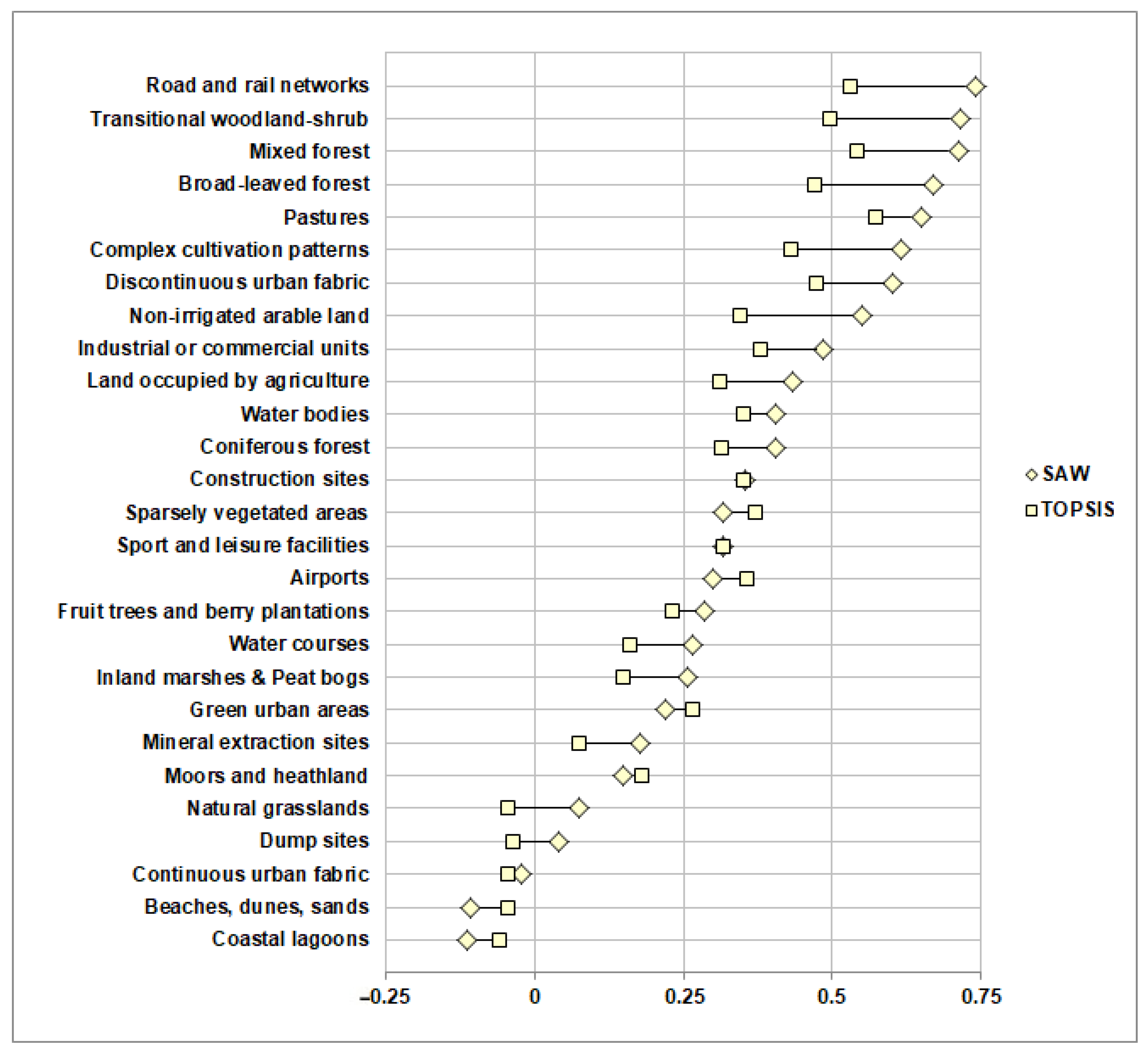
- Feranec, J.; Jaffrain, G.; Soukup, T.; Hazeu, G. Determining changes and flows in European landscapes 1990–2000 using CORINE land cover data. Appl. Geogr. 2010, 30, 19–35. [Google Scholar] [CrossRef]
- European Environmental Agency. CORINE Land Cover—Copernicus Land Monitoring Service. Available online: https://land.copernicus.eu/pan-european/corine-land-cover (accessed on 16 March 2020).
- European Environmental Agency. CORINE Land Cover Nomenclature Guidelines. Available online: https://land.copernicus.eu/user-corner/technical-library/corine-land-cover-nomenclature-guidelines/html (accessed on 12 November 2020).
- Akoglu, H. User’s guide to correlation coefficients. Turk. J. Emerg. Med. 2018, 18, 91–93. [Google Scholar] [CrossRef] [PubMed]
- Maleika, W. Inverse distance weighting method optimization in the process of digital terrain model creation based on data collected from a multibeam echosounder. Appl. Geomat. 2020, 12, 397–407. [Google Scholar] [CrossRef]
- Chen, F.-W.; Liu, C.-W. Estimation of the spatial rainfall distribution using inverse distance weighting (IDW) in the middle of Taiwan. Paddy Water Environ. 2012, 10, 209–222. [Google Scholar] [CrossRef]
- Luque, S.; Saura, S.; Fortin, M.-J. Landscape connectivity analysis for conservation: Insights from combining new methods with ecological and genetic data. Landsc. Ecol. 2012, 27, 153–157. [Google Scholar] [CrossRef]
- Kučas, A. Web Map of Ungulate-Vehicle Collision Hotspots in Lithuania 2002–2017. Available online: https://www.arcgis.com/apps/MapJournal/index.html?appid=d81195212a4b4bcc9c5aab34a0037609 (accessed on 16 March 2020).
- Kučas, A.; Balčiauskas, L. Mammal Roadkill Clusters, Corridors, Pathways and Habitats. [WWW Document]. Mendeley Data, V1. Available online: https://doi.org/10.17632/4c58n345h5.1 (accessed on 1 May 2021).
- Lithuanian Road Administration under the Ministry of Transport and Communications. Annual Average Daily Traffic Volumes in Lithuania. Available online: https://lakd.lrv.lt/en/sector-activities/traffic-volumes (accessed on 16 March 2020).
- Hortal, J.; Triantis, K.A.; Meiri, S.; Thébault, E.; Sfenthourakis, S. Island Species Richness Increases with Habitat Diversity. Am. Nat. 2009, 174, E205–E217. [Google Scholar] [CrossRef] [Green Version]
- Hernández-Quiroz, N.S.; Badano, E.I.; Barragán-Torres, F.; Flores, J.; Pinedo-Álvarez, C. Habitat suitability models to make conservation decisions based on areas of high species richness and endemism. Biodivers. Conserv. 2018, 27, 3185–3200. [Google Scholar] [CrossRef]
- Ramp, D.; Wilson, V.K.; Croft, D.B. Assessing the impacts of roads in peri-urban reserves: Road-based fatalities and road usage by wildlife in the Royal National Park, New South Wales, Australia. Biol. Conserv. 2006, 129, 348–359. [Google Scholar] [CrossRef]


| Species | Mapped (MVC) |
|---|---|
| Roe deer (Capreolus capreolus) | 10,741 |
| Wild boar (Sus scrofa) | 1416 |
| Moose (Alces alces) | 1340 |
| Raccoon dog (Nyctereutes procyonoides) | 1331 |
| Eastern European hedgehog (Erinaceus concolor) | 993 |
| Red fox (Vulpes vulpes) | 829 |
| European hare (Lepus europaeus) | 456 |
| Marten (Martes sp.) | 405 |
| Red deer (Cervus elaphus) | 248 |
| European polecat (Mustela putorius) | 160 |
| Badger (Meles meles) | 89 |
| Pine marten (Martes martes) | 40 |
| Beaver (Castor fiber) | 25 |
| Red squirrel (Sciurus vulgaris) | 30 |
| American mink (Neovison vison) | 26 |
| European mole (Talpa europaea) | 19 |
| Stone marten (Martes foina) | 14 |
| Eurasian otter (Lutra lutra) * | 13 |
| Fallow deer (Dama dama) | 11 |
| Norway rat (Rattus norvegicus) | 6 |
| European bison (Bison bonasus) * | 6 |
| Grey wolf (Canis lupus) | 3 |
| Bank vole (Myodes glareolus) | 3 |
| Lynx (Lynx lynx) * | 1 |
| Stoat (Mustela erminea) * | 2 |
| Least weasel (Mustela nivalis) | 2 |
| Common shrew (Sorex araneus) | 2 |
| Yellow-necked mouse (Apodemus flavicollis) | 2 |
| Muskrat (Ondatra zibethicus) | 2 |
| Water shrew (Neomys fodiens) | 1 |
| Mountain hare (Lepus timidus) * | 1 |
| Black rat (Rattus rattus) | 1 |
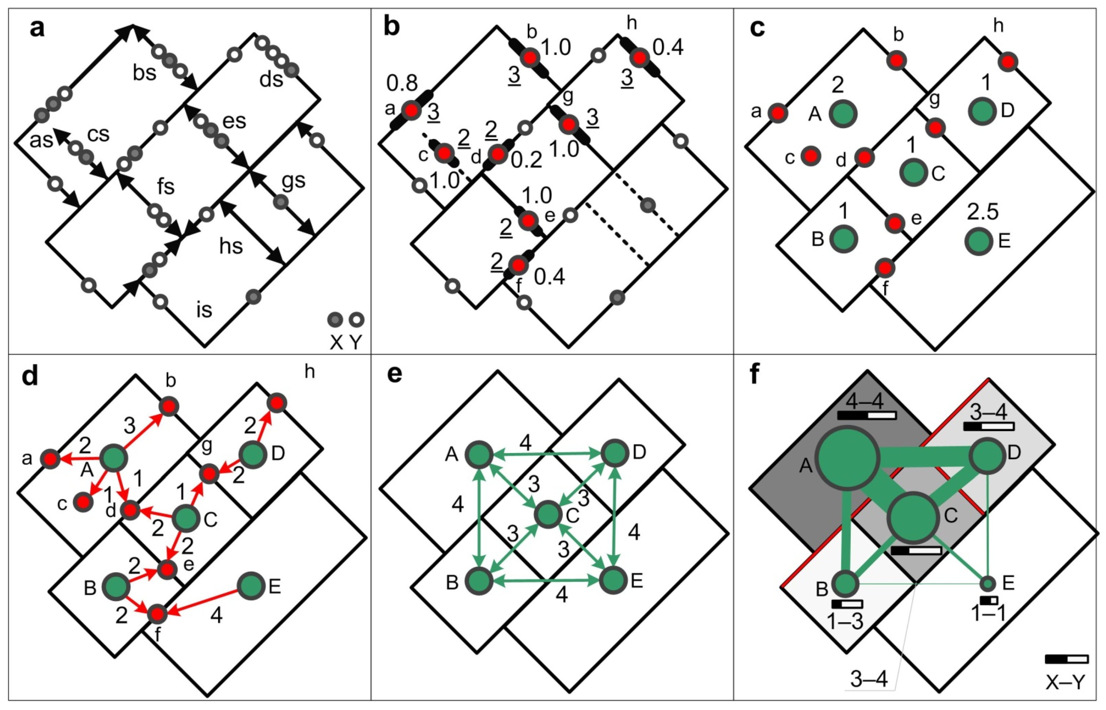
| Criteria Name * | Variable | Habitat Patches | Objective Function | Weight (Index) ** | ||||
|---|---|---|---|---|---|---|---|---|
| A | B | C | D | E | ||||
| Total number of collisions within adjacent clusters i (b) | count | 10.0 | 4.0 | 7.0 | 7.0 | 2.0 | Max | 0.102 |
| Average strength of adjacent clusters ii (b) | index | 0.8 | 0.7 | 0.7 | 0.7 | 0.4 | Max | 0.098 |
| Total length of adjacent clusters ii (b) | km | 10.0 | 4.0 | 7.0 | 6.0 | 2.0 | Max | 0.103 |
| Number of species within adjacent clusters iii (b) | count | 2.0 | 2.0 | 2.0 | 2.0 | 2.0 | Max | 0.097 |
| Habitat patch area i (c) | ha | 2.0 | 1.0 | 1.0 | 1.0 | 2.5 | Max | 0.102 |
| Number of adjacent clusters/pathways ii (d) | count | 4.0 | 2.0 | 3.0 | 2.0 | 1.0 | Max | 0.102 |
| Total length of adjacent pathways ii (d) | km | 7.0 | 4.0 | 5.0 | 4.0 | 4.0 | Min | 0.098 |
| Number of adjacent corridors i (e) | count | 3.0 | 3.0 | 4.0 | 3.0 | 3.0 | Max | 0.100 |
| Total length of adjacent corridors i (e) | km | 11.0 | 11.0 | 12.0 | 11.0 | 11.0 | Min | 0.097 |
| Total area of adjacent habitat patches i (e) | ha | 3.0 | 5.5 | 6.5 | 5.5 | 3.0 | Max | 0.101 |
| SAW values (f) *** | index | 0.86 | 0.72 | 0.82 | 0.78 | 0.64 | ||
| TOPSIS values (f) *** | index | 0.69 | 0.37 | 0.58 | 0.48 | 0.32 | ||
| Corridor Identification (Figure 2e Cases) | Average SAW Value * | Average TOSPIS Value * |
|---|---|---|
| A–B | 0.78 | 0.53 |
| A–C | 0.84 | 0.63 |
| B–C | 0.77 | 0.47 |
| A–D | 0.82 | 0.59 |
| C–D | 0.80 | 0.53 |
| D–E | 0.71 | 0.40 |
| E–C | 0.73 | 0.45 |
| B–E | 0.68 | 0.35 |
| Criteria Name * | Weight (Index) |
|---|---|
| Total number of collisions within adjacent clusters i (b) | 0.107 |
| Average strength of adjacent clusters ii (b) | 0.085 |
| Total length of adjacent clusters ii (b) | 0.104 |
| Number of species within adjacent clusters iii (b) | 0.099 |
| Habitat patch area i (c) | 0.105 |
| Number of adjacent clusters/pathways ii (d) | 0.103 |
| Total length of adjacent pathways ii (d) | 0.109 |
| Number of adjacent corridors i (e) | 0.088 |
| Total length of adjacent corridors i (e) | 0.103 |
| Total area of adjacent habitat patches i (e) | 0.098 |
| Independent ± SE\Dependent | SAW | TOPSIS |
|---|---|---|
| Intercept | 0.208791 ± 0.000 **** | 0.4098186 ± 0.000 **** |
| bdiscontinuous urban fabric | −0.000003 ± 0.393 NS | −0.0000002 ± 0.896 NS |
| broad and rail networks and associated land | 0.000019 ± 0.000 **** | 0.0000043 ± 0.025 ** |
| bpastures | −0.000002 ± 0.074 * | −0.0000004 ± 0.251 NS |
| bcomplex cultivation patterns | −0.000001 ± 0.481 NS | −0.0000004 ± 0.502 NS |
| bbroad-leaved forest | 0.000002 ± 0.005 *** | 0.0000000 ± 0.871 NS |
| bmixed forest | −0.000003 ± 0.053 * | 0.0000006 ± 0.343 NS |
| btransitional woodland–shrub | 0.000015 ± 0.001 *** | −0.0000051 ± 0.003 ** |
| bMustela putorius | 0.003593 ± 0.189 NS | 0.0023776 ± 0.016 ** |
| bMartes sp. | 0.000106 ± 0.939 NS | 0.0011592 ± 0.021 ** |
| bLepus europaeus | 0.003250 ± 0.041 ** | 0.0000625 ± 0.912 NS |
| bVulpes vulpes | 0.001217 ± 0.269 NS | 0.0010652 ± 0.007 *** |
| bErinaceus concolor | 0.001905 ± 0.016 ** | 0.0003457 ± 0.222 NS |
| bNyctereutes procyonoides | −0.000047 ± 0.928 NS | 0.0003072 ± 0.106 NS |
| bAlces alces | 0.000058 ± 0.898 NS | 0.0005224 ± 0.001 **** |
| bSus scrofa | 0.002013 ± 0.001 *** | 0.0005760 ± 0.006 *** |
| bCapreolus capreolus | 0.000803 ± 0.000 **** | 0.0004290 ± 0.000 **** |
| F(16,226) | 98.02606 ± 0.000 **** | 132.64396 ± 0.000 **** |
| R2 | 0.874 | 0.904 |
Publisher’s Note: MDPI stays neutral with regard to jurisdictional claims in published maps and institutional affiliations. |
© 2021 by the authors. Licensee MDPI, Basel, Switzerland. This article is an open access article distributed under the terms and conditions of the Creative Commons Attribution (CC BY) license (https://creativecommons.org/licenses/by/4.0/).
Share and Cite
Kučas, A.; Balčiauskas, L. Roadkill-Data-Based Identification and Ranking of Mammal Habitats. Land 2021, 10, 477. https://doi.org/10.3390/land10050477
Kučas A, Balčiauskas L. Roadkill-Data-Based Identification and Ranking of Mammal Habitats. Land. 2021; 10(5):477. https://doi.org/10.3390/land10050477
Chicago/Turabian StyleKučas, Andrius, and Linas Balčiauskas. 2021. "Roadkill-Data-Based Identification and Ranking of Mammal Habitats" Land 10, no. 5: 477. https://doi.org/10.3390/land10050477